Does Future Climate Bring Greater Streamflow Simulated by the HSPF Model to South Korea?


1
Prediction Research Department, Climate Services and Research Division, APEC Climate Center, Busan 48058, Korea
2
Civil Engineering, Dong-a University, Busan 49315, Korea
3
Climate Prediction Department, Climate Services and Research Division, APEC Climate Center, Busan 48058, Korea
4
Convergence Center for Watershed Management, Integrated Watershed Management Institute, Suwon 16489, Korea
*
Author to whom correspondence should be addressed.
Water 2020, 12(7), 1884; https://doi.org/10.3390/w12071884
Submission received: 20 April 2020
/
Revised: 25 June 2020
/
Accepted: 27 June 2020
/
Published: 1 July 2020
(This article belongs to the Special Issue Study for Ungauged Catchments—Data, Models and Uncertainties)
Abstract
:Evaluating the impact of climate change on water resources is necessary for improving water resource management and adaptation measures at the watershed level. This study evaluates the impact of climate change on streamflow in South Korea using downscaled climate change information based on the global climate model (GCM) and hydrological simulation program–FORTRAN model. Representative concentration pathway (RCP) scenarios 4.5 and 8.5 W/m2 were employed in this study. During the distant future (2071–2099), the flow increased by 15.11% and 24.40% for RCP scenarios 4.5 and 8.5 W/m2, respectively. The flow is highly dependent on precipitation and evapotranspiration. Both precipitation and evapotranspiration increased, but the relative change of precipitation was greater than the relative change of evapotranspiration. For this reason, the flow would show a significant increase. Additionally, for RCP 8.5 W/m2, the variability of the flow according to the GCM also increased because the variability of precipitation increased. Moreover, for RCP 8.5 W/m2, the summer and autumn flow increased significantly, and the winter flow decreased in both scenarios. The variability in autumn and winter was so great that the occurrence of extreme flow could intensify further. These projections indicated the possibility of future flooding and drought in summer and winter. Regionally, the flow was expected to show a significant increase in the southeastern region. The findings presented for South Korea could be used as primary data in establishing national climate change adaptation measures.
1. Introduction
The severity of the impact of climate change caused by global warming on local water resources has been highlighted by various studies [1]. Climate change causes the peak flow of streams to increase, and the seasonal circulation of streamflow can significantly impact agricultural and flood disaster management [2]. Evaluating the future flow change of river subwatersheds using the global climate model (GCM) indicated that climate change increases high flow and decreases low flow, thereby increasing the variability of seasonal streamflow as a whole [3]. During the past decade, research on water resources has assessed future hydrological conditions and has shown that adapting to climate change is an essential strategy for water resource management [1,4].
Evaluating the impact of climate change on water resources is necessary to improve water resource management and adaptation measures at the watershed level [2]. As water resources are related to a breadth of fields, including everyday life, the environment, industry, and society, evaluating how water resources affect regions of interest by forecasting future changes is important. In particular, producing and analyzing hydrological scenarios at the national level according to climate change is needed to establish a comprehensive national plan for long-term water resources.
A top–down approach is used as a method to forecast future hydrological status. The top–down method predicts changes to water resources by applying future climate information that has been produced by climate models that are appropriate for the study watershed to hydrological models [5,6]. Therefore, when assessing the impact of water resources due to climate change, selecting a hydrological model suitable for the purpose of evaluation and the study watershed is important. It was necessary that the hydrological model used in this study was able to evaluate changes in the hydrological cycle of watersheds using downscaled climate information (precipitation, maximum temperature, and minimum temperature) based on the fifth assessment report (AR5) scenario. The appropriate hydrological model needed to offer flexibility in inputting data so that reliable runoff analysis could be performed using limited climate information. In addition, considering the hydrological circulation analysis of watersheds, the watershed characteristics needed to be able to reflect regionally different characteristics depending on the elevation, land cover, and slope.
In this study, the hydrological simulation program–FORTRAN (HSPF) model, a widely used model worldwide, was selected as the runoff model for the production of hydrological scenarios. The HSPF model is a continuous, semi-distributed watershed model designed to simulate water quantity and quality. As an advantage of the semi-distributed model, a geographic information system (GIS) can be used to directly estimate the parameters of watershed topography and soil characteristics. It is also suitable for evaluating the impact of climate change due to its faster computation speed compared with the distributed model.
Several researchers have conducted hydrological analysis using the HSPF model. Studies utilizing HSPF models to simulate runoff when considering climate change have been conducted in various regions. Zhou et al. (2017) simulated runoff in the context of climate change in the Jianfengling watershed in China [7], while Göncü and Albek (2010) simulated runoff from rivers and reservoirs due to climate change [8]. Albek et al. (2004) conducted a runoff simulation to study the impact of climate change in the Seydi Suyu watershed in Turkey [9].
Several studies have also analyzed runoff simulated by the HSPF model and have compared the results of the HSPF model with those simulated using other hydrological models. A number of comparisons have been made with the Soil and Water Assessment Tool (SWAT) models that are used all over the world, and studies comparing the results of simulations using statistical techniques have also been conducted [10,11,12,13].
Several studies have evaluated the applicability of HSPF to watersheds in South Korea. Most studies have conducted hydrological impact assessments on subwatersheds. Kim and Kim (2018) explored the applicability of a HSPF model runoff estimation to subwatersheds located in the Namgang Dam watershed [14], and Hwang (2010) estimated the runoff by each subwatershed for Namgang and Hwanggang watersheds using the HSPF model [15]. Kim et al. (2009) assessed the applicability of the HSPF model to the Baran reservoir watershed through the model’s calibration and validation [16], and Kim and Park (2004) estimated the runoff and contaminant concentrations in the Baran reservoir watershed using the HSPF model [17]. Also, several studies have employed the HSPF model to assess the impact of water resources on climate change. Bae et al. (2011) showed the differences in runoff change under climate change scenarios in the Chungju Dam basin [5]. Shin et al. (2016) found the alteration of hydrologic regimes under climate change for seven Korean catchments [6].
Looking at the previous studies on South Korea, the hydrological changes in the future are clear. During the rainy season, the rate of flow increase was significantly higher. Flood damage is expected due to increased peak runoff. In addition, there was a noticeable increase in runoff in the distant future [5]. However, in most of the research, the spatial extent is limited to subwatersheds. Thus, there is a lack of information on spatial differences in national level runoff change. The spatial distribution of runoff changes is not uniform across the basin [2]. Therefore, to establish a comprehensive national plan for long-term water resource for South Korea, a study that analyzes hydrological changes across the entire watersheds is needed.
The objective of this study was to evaluate the impact of climate change on streamflow in South Korea using GCM-based downscaled climate change information and the HSPF model. The original temporal resolution of the future hydrological scenario was daily data, and the spatial resolution was targeted at 109 mid-size watersheds in South Korea. The final resolution was targeted to South Korea and was analyzed for long-term streamflow according to climate change by combining the year, season, and month. The streamflow simulated in this study was natural streamflow without human-induced mechanisms.
2. Materials and Methods
The HSPF model and 13 climate change scenarios were used to assess the impact of climate change on streamflow. The past hydrological climate data and topographical data were constructed for the HSPF model setup. After completing the model setup, the HSPF model calibration and validation were performed for six representative dams’ watersheds. The parameter localization for the remaining mid-size watersheds were performed using optimized parameters for six dams. Then, future streamflow projection over South Korea were simulated using 13 climate change scenarios.
2.1. HSPF Model
The HSPF model is a semi-distributed continuous model for watershed hydrology and water quality that was developed by the U.S. Environmental Protection Agency. The HSPF model employs hydrologic response units (HRUs) that have homogeneous parameters and meteorological input data to segment land surface areas. In this study, HRUs were sorted into pervious-area land (PERLND) and impervious-area land (IMPLND). The PERLND module simulated runoff from the permeable area in the watershed and the IMPLND module simulated runoff from the impermeable area in the watershed. HRUs flowed into reaches (RCHRES), which represent stream channels, lakes, and reservoirs. The RCHRES module received the results of the PERLND and IMPLND modules as input data and performed hydraulic and pollutant simulation in the water body. PERLND, IMPLND, and RCHRES were the three main modules in the HSPF model. The HSPF model simulated rainfall interception, evapotranspiration, soil retention, surface runoff, interflow, groundwater, snowmelt, pH, temperature, dissolved oxygen, nutrients, biochemical oxygen demand, pesticides, and Escherichia coli (E. coli), among other parameters. It is possible to simulate hydrological and water quality in various scales and complex watersheds [18,19,20].
South Korea has topographical features in which rural and urban areas are diversely mixed. Therefore, it is necessary to consider hydrological considerations for various land use, permeable, and impervious areas. The HSPF model can be simulated for both permeable and impervious areas, making it suitable for multi-watersheds with mixed urban and rural watersheds. Besides, the HSPF model can simulate a wide range of organic and inorganic substances in complex watersheds, so that it can analyze not only the effects of climate change on long-term streamflow but also water quality.
2.2. HSPF Model Setup
2.2.1. Hydrological Climate Data Construction
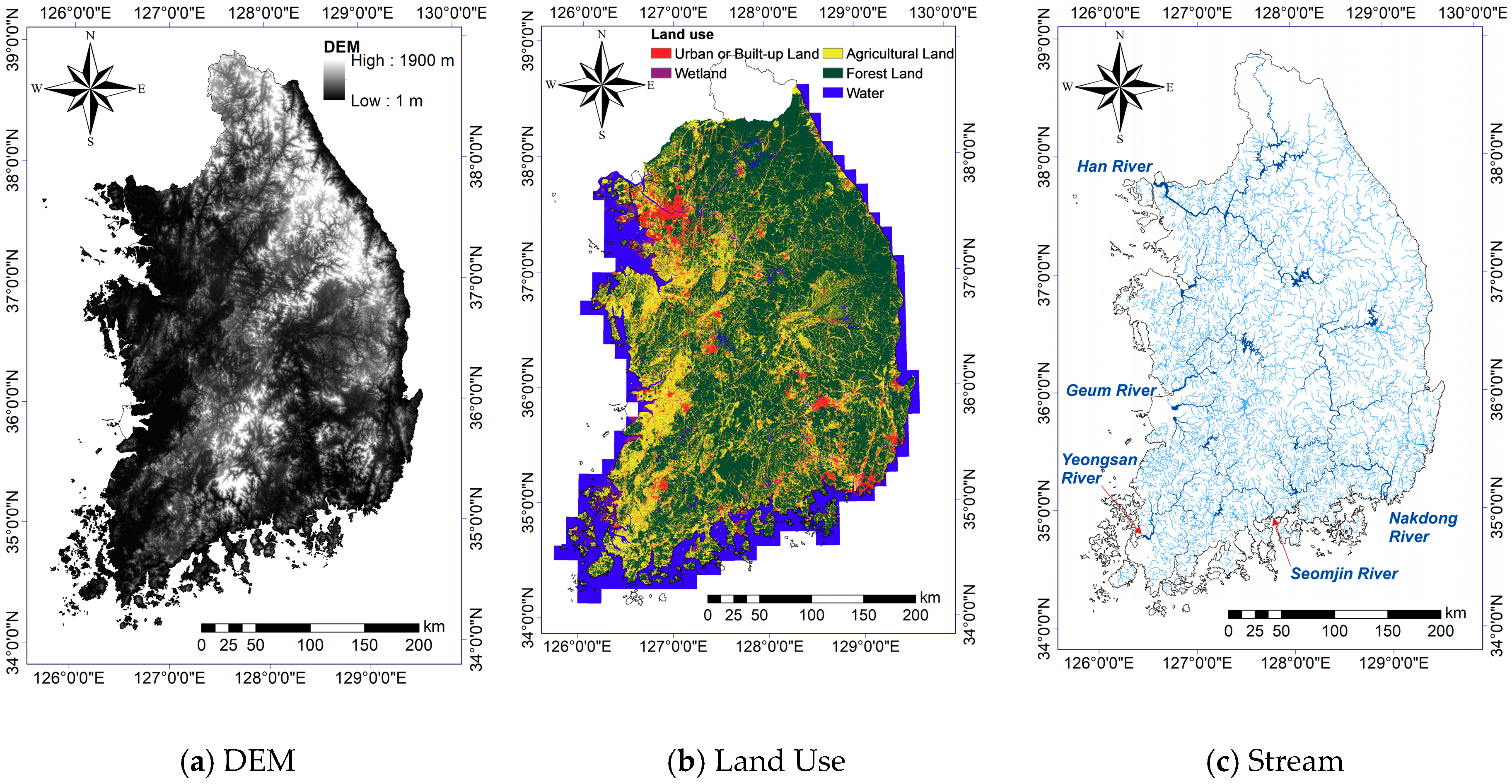
The HSPF model’s historical observed climate data were constructed from 60 automated synoptic observing systems (ASOSs) operated by the Korea Meteorological Administration. South Korea was divided into 109 mid-size watersheds to simulate long-term streamflow in South Korea. A Thiessen polygon was established for 60 ASOSs, and the data for each station were converted into area values of 109 mid-size watersheds. Figure 1 illustrates the study area and the 60 ASOS locations used in this study.
The dam’s historical observed inflow data were constructed for the parameter calibration of the HSPF model. These inflow data can be found in the water management information system (WAMIS; http://www.wamis.go.kr/ENG) and MyWater (https://www.water.or.kr) sites. Natural flow data with little artificial interference, such as inflow data from the upper watersheds of dams, is ideal for reliable parameter estimation and has been utilized in previous studies. In particular, the inflow data provided by WAMIS has been applied with quality control and has been judged to be highly reliable.
Future climate data were constructed using 13 GCMs to produce future hydrological scenarios. The 13 GCMs used in this study were statistically downscaled data for 60 ASOS using spatial disaggregation quantile delta mapping (SDQDM) [21,22]. The 13 GCMs provided precipitation, maximum temperature, and minimum temperature, and some GCMs provided additional climate variables. As with the observed climate data, climate data from 60 ASOS were converted to area values of 109 mid-size watersheds using the Thiessen polygon. The simulation period was divided into four periods for the representative concentration pathways (RCPs), scenarios 4.5 and 8.5: S0 (reference: 1976–2005), S1 (near future: 2011–2040), S2 (mid–century: 2041–2070), and S3 (distant future: 2071–2099). Table 1 provides information on the 13 GCMs used in this study and the variables.
Climate input data should be constructed in watershed data management (WDM) format to simulate flow data using the HSPF model. The type of data required can vary depending on the target variable. However, in general, flow is simulated by constructing the data of precipitation, temperature, wind speed, solar radiation, potential evapotranspiration, evaporation, dew point, and clouds. As the HSPF internal algorithm was initially set to run on an hourly interval in this study, it was simpler to simulate the HSPF model using hourly data. In general, except for precipitation, obtaining hourly data was challenging; therefore, hourly climate data were calculated using the interval algorithm by WDM UTIL, which disaggregates daily data into hourly data. In this study, 13 GCM climate input data were constructed for RCP scenarios 4.5 and 8.5 using the WDM UTIL time disaggregation algorithm. The potential evapotranspiration was estimated using the Hargreaves equation, which uses the maximum and minimum temperatures [23,24], as follows Equation (1):
where is the potential evapotranspiration (mm/day), and are the maximum and minimum values of air temperature (°C), and is the extraterrestrial radiation (mm/day) outside the earth’s atmosphere. , which was initially expressed as , was converted to mm/day using the conversion factor 0.408 [25].
2.2.2. Topographical Data Construction
Topographical data for the HSPF model simulation were generated using better assessment science integrating point and nonpoint sources (BASINS). BASINS is a watershed management system developed by the United States Environmental Protection Agency (USEPA) to synthesize watersheds and point and nonpoint sources for the efficient operation of total maximum daily load, as well as to facilitate access to vast amounts of GIS data. BASINS can build input data using various GIS files. The GIS files used in this study, which included the digital elevation model (DEM) of 30 m grid size, land use map, watershed map, and stream map, were constructed using WAMIS and Ministry of Environment data. Along with the GIS data provided, DEM was divided into subwatersheds with the BASINS automatic delineation tool. After the subwatershed delineation, land use was used to classify areas into urban or built-up land, agricultural land, forest land, wet land, and water (Figure 2). In total, 109 mid-size watersheds were used in this study.
2.3. HSPF Model Calibration and Validation
Parameter calibration and validation of the HSPF model were conducted on the upper watersheds of dams. The parameters of the HSPF model were evaluated for six representative dams’ watersheds: the Goesan Dam, Andong Dam, Imha Dam, Hapcheon Dam, Yongdam Dam, and Seomjin River Dam, where daily flow data were established (Table 2). Table 3 shows the types and ranges of the HSPF parameters related to the flow simulation.
2.4. HSPF Model Evaluation
The coefficient of determination (R2), Nash–Sutcliffe efficiency (NSE), and percent bias (PBIAS) were used Equations (2)–(4) to evaluate the model. R2 evaluated the correlation between the observed and simulated values and was expressed as a value between 0 and 1, which indicated that there was a completely linear relationship. NSE is a normalization of the relative magnitude of residual variance between the observed and simulated value calculated in the range of −∞ to 1; NSE = 1 indicates a perfect match with the observed value. PBIAS calculates the average tendency of the simulated data to be greater or less than the observed data. Positive numbers are overestimated, and negative numbers are underestimated. Table 4 shows the performance evaluation criteria of each statistic used in this study.
and denote the observed data and simulated data, respectively.
3. Results and Discussion
3.1. HSPF Model Calibration and Validation Result
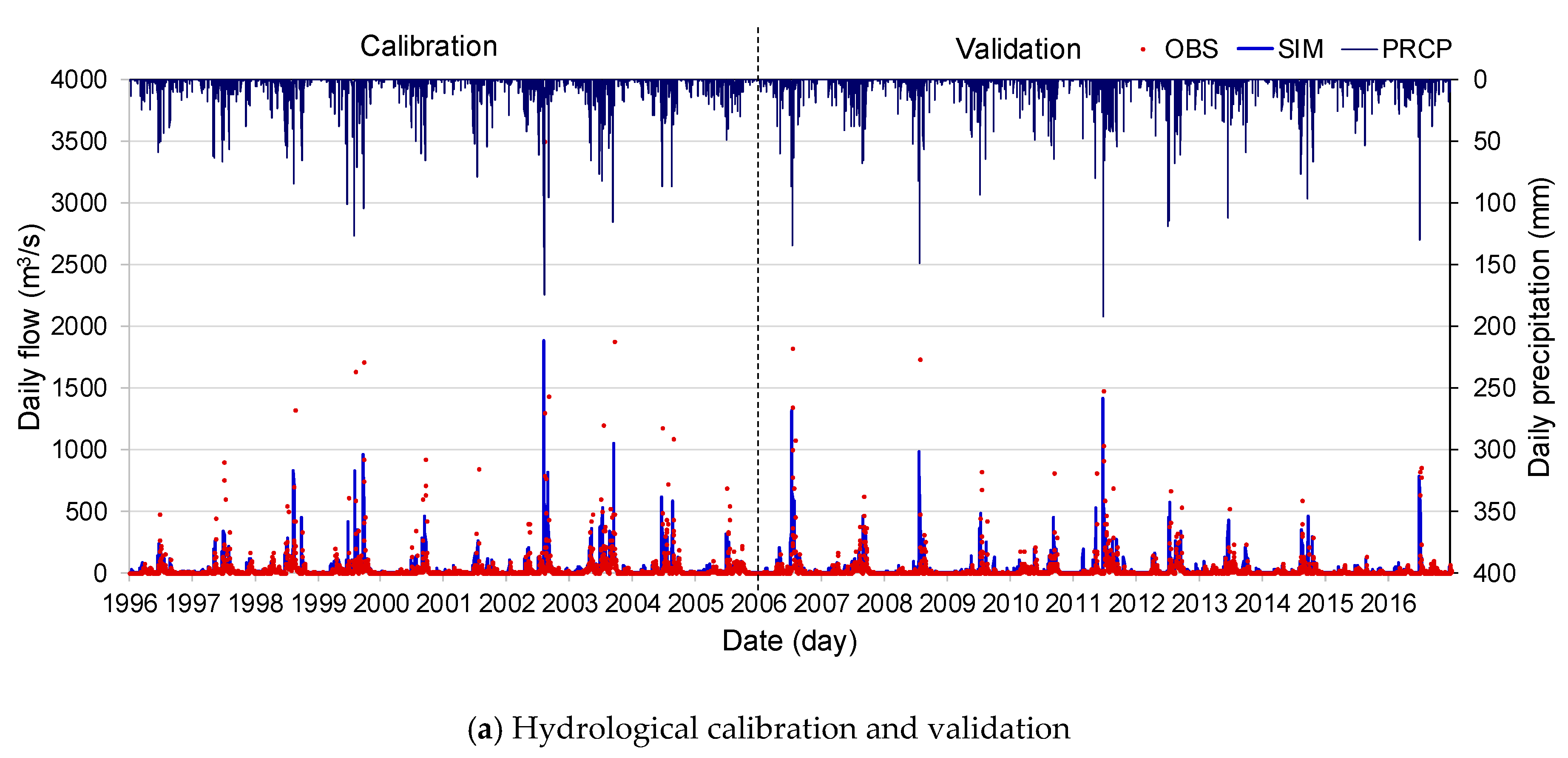
As a result of the calibration and validation, the R2 was 0.6670–0.8234, the NSE was 0.6679–0.8201, and the PBIAS was –16.0404–2.2801% for the daily data from the six dam watersheds. It was found that the NSE of the Andong Dam and Yongdam Dam was over 0.8, which was a good result. For the Yongdam Dam, the PBIAS of the correction period was −16.0404%, which was an underestimation of the actual value. After comprehensively assessing the range of statistics, it was determined that the parameter calibration and validation of the HSPF model had been adequately performed in the six dam watersheds (Table 5). Figure 3 shows the representative results of the calibration and validation of the Andong Dam.
3.2. Future Climate and Long-term Flow Projection and Relative Change Analysis Over South Korea
3.2.1. Future Climate and Long-Term Flow Projection over South Korea
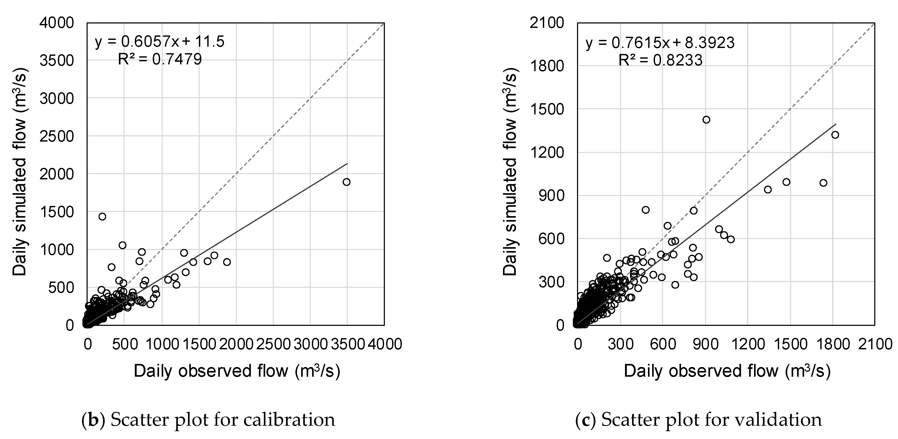
Projections for the climate and hydrological variables from 1976 to 2099 were analyzed for 13 climate change scenarios. Figure 4 shows the average and variability of 13 climate change scenarios for precipitation, temperature, evapotranspiration, and flow for RCP scenarios 4.5 and 8.5. In Figure 4, the red area indicates the reference period (1976–2005) reflecting the observed data, the green area indicates RCP scenario 4.5, and the blue area is RCP scenario 8.5. Precipitation and flow were volatile in RCP scenarios 4.5 and 8.5 over time and were more volatile in RCP 8.5 after 2050. The difference between the average temperature and potential evapotranspiration between RCP scenarios 4.5 and 8.5 was obvious over time. Their variability was relatively low compared to precipitation and flow. The 30-year average annual precipitation for the reference period (S0: 1976–2005) was 1306.8 mm, the temperature was 12.4 °C, the potential evapotranspiration was 1055.6 mm, and the flow was 72,969.4 m³. In the future third period (S3: 2071–2099) for RCP 8.5, the 30-year average annual precipitation was expected to increase to 1540.1 mm, the temperature to 16.5 °C, the potential evapotranspiration to 1187.3 mm, and the flow to 90,826.7 m³. Table 7 summarizes the 30-year average for the reference and three future periods for RCP scenarios 4.5 and 8.5 in South Korea.
3.2.2. Relative Change Analysis of Future Climate and Long-Term Flow over South Korea
Table 8 shows the relative change of 30-year average annual precipitation, temperature, potential evapotranspiration, and flow for future periods (S1: 2011–2040, S2: 2041–2070, and S3: 2071–2099) compared with the reference period (1976–2005) for RCP scenarios 4.5 and 8.5. Precipitation was projected to increase by 11.32% for RCP 4.5 and 17.82% for RCP 8.5 by S3. The temperature was expected to increase steadily by 2.29 °C for RCP 4.5 and 4.07 °C for RCP 8.5 by 2099. In general, RCP 8.5 was projected to increase more than RCP 4.5. The potential evapotranspiration was expected to increase by 6.88% for RCP 4.5 and 12.48% for RCP 8.5. The flow was expected to increase by 15.11% for RCP 4.5 and 24.40% for RCP 8.5. During S3 for RCP 8.5, compared with the increase in precipitation to 17.82%, the potential evapotranspiration increased by only 12.48%. Both precipitation and evapotranspiration increased, but the relative change of precipitation was greater than the relative change of evapotranspiration. And Zhang et al. (2019) indicated that annual runoff was dominated by changes in precipitation than changes in temperature [3]. For this reason, the flow, which is highly dependent on precipitation and evapotranspiration, would show a significant increase.
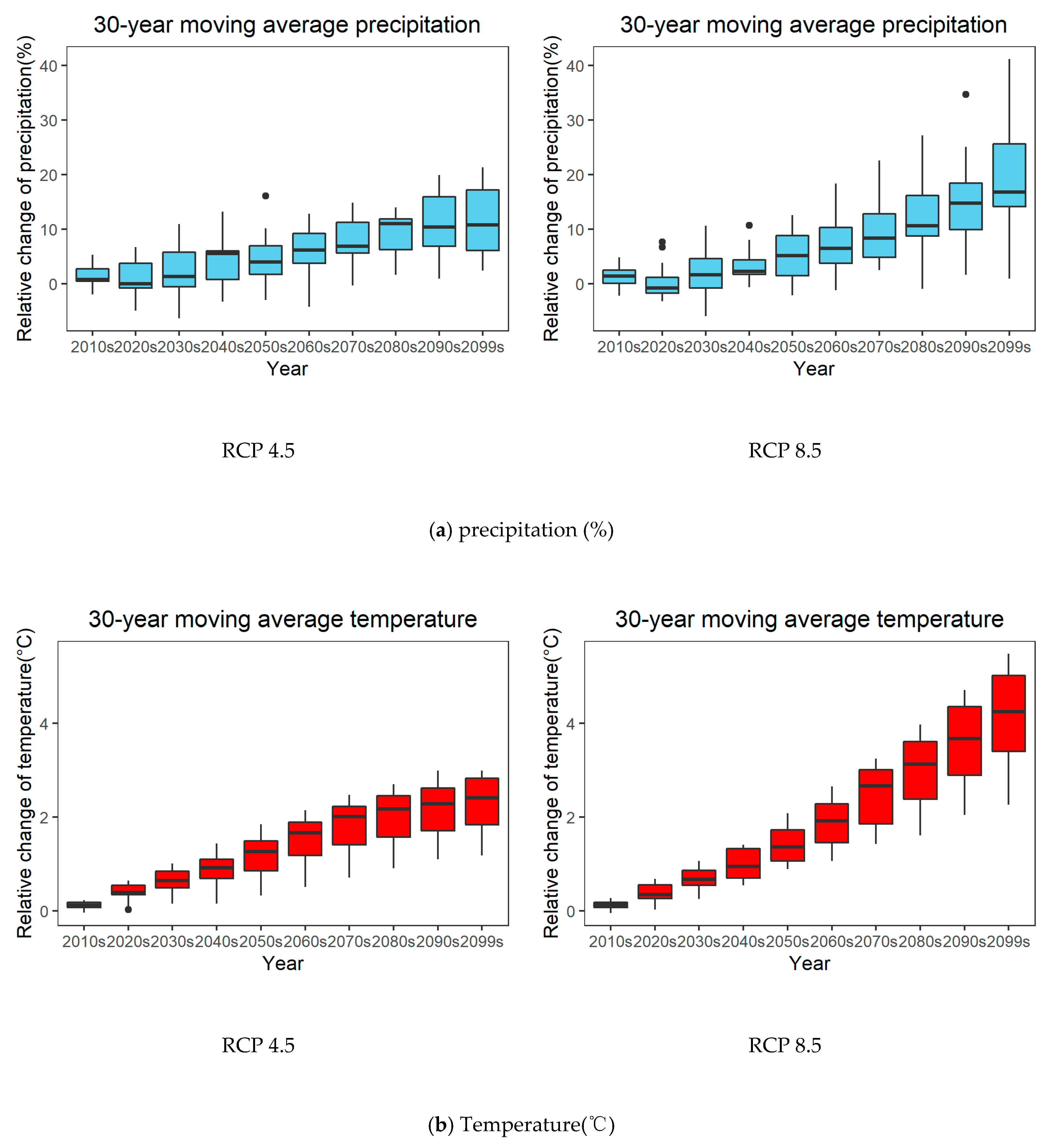
Figure 5 shows the box plot of the relative change of the 30-year moving average annual precipitation, temperature, potential evapotranspiration, and flow compared with the reference period for RCP scenarios 4.5 and 8.5 using 13 GCMs as a box plot every 10 years. The relative change was calculated using the reference 30-year average (S0: 1976–2005) and the 30-year average for the future periods (2010s: 1981–2010; 2020s: 1991–2020; 2030s: 2001–2030; 2040s: 2011–2040; 2050s: 2021–2050; 2060s: 2031–2060; 2070s: 2041–2070; 2080s: 2051–2080; 2090s: 2061–2090; and 2099s: 2071–2099). The quartile range, minimum, maximum, and median are shown for each variable. The temperature and potential evapotranspiration tended to increase steadily. The variability of the potential evapotranspiration increased toward the second half of the future. Notably, it showed negative-skewed characteristics as the second half of the future approached. The precipitation also showed an increasing tendency. In RCP 8.5, the variability in precipitation according to GCM increased noticeably in the second half of the future. In RCP 8.5, the flow tended to increase steadily toward the future, and the variability also increased.
3.2.3. Relative Change Analysis of Future Seasonal and Monthly Flow over South Korea
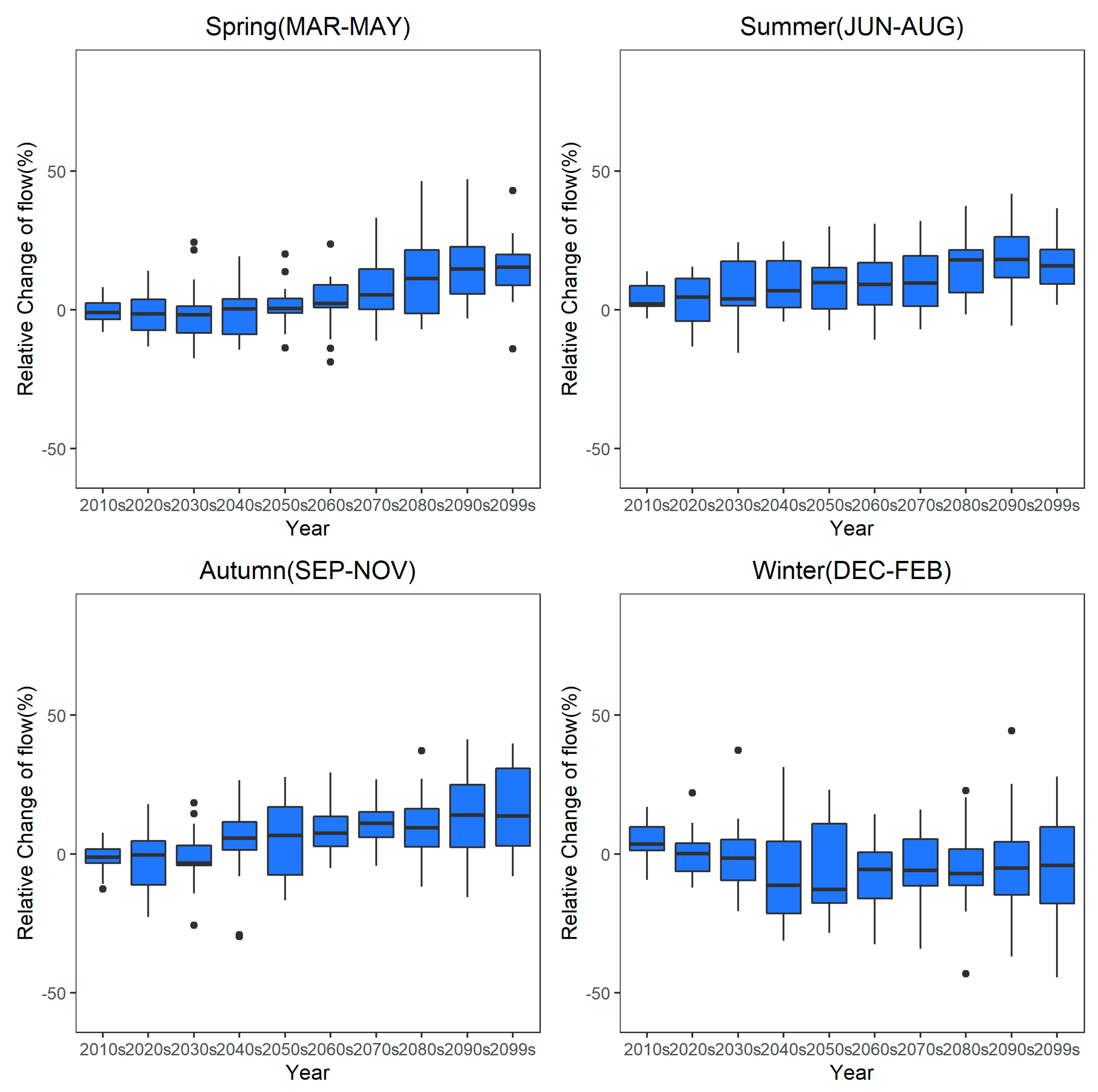
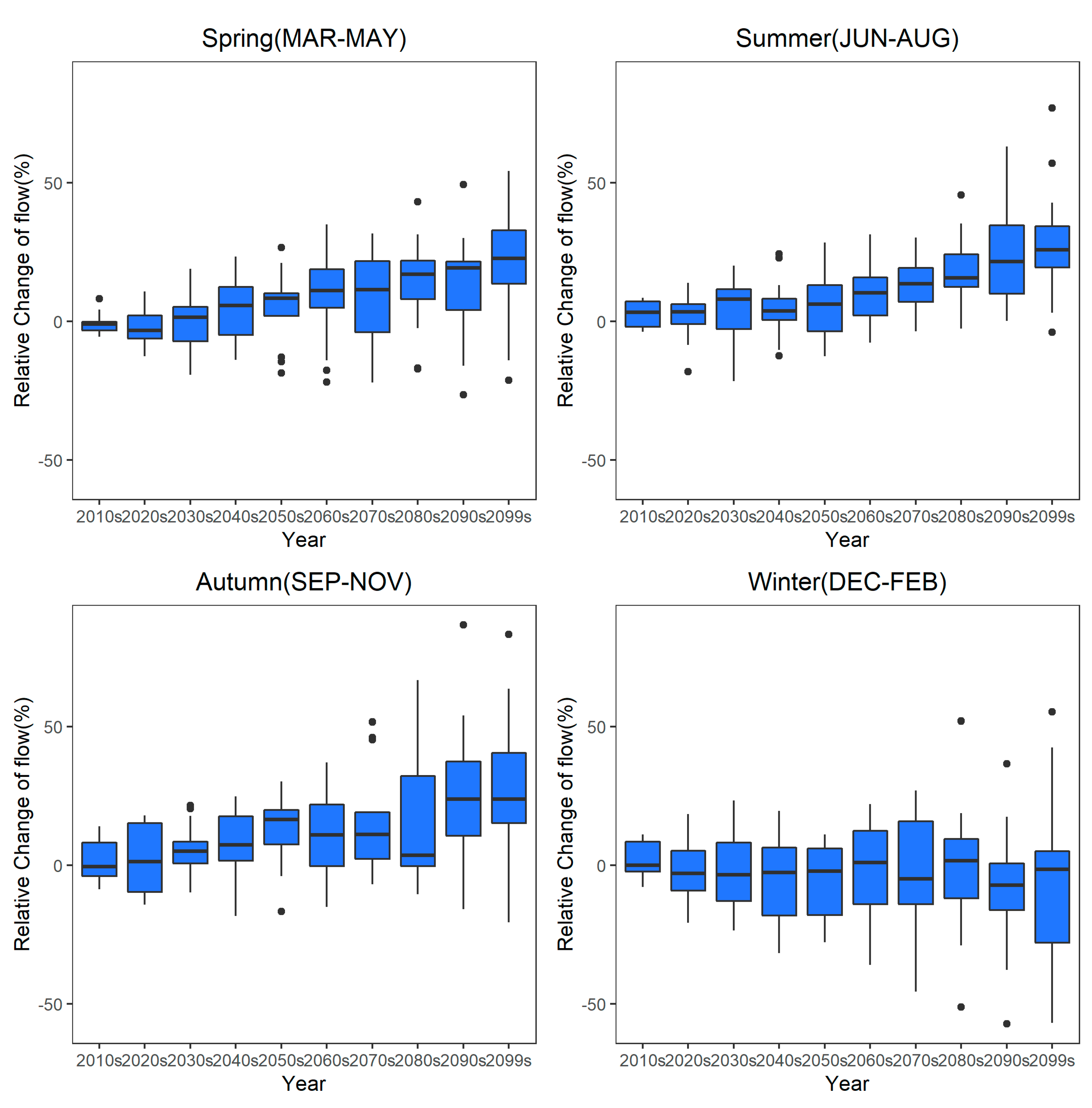
Table 9 shows the relative change of the seasonal flow. Figure 6 and Figure 7 show the relative change of the 30-year moving average seasonal flow compared with the reference period (1976–2005) for RCP scenarios 4.5 and 8.5 using 13 GCMs in a box plot every 10 years. In S3 (2071–2099), the relative change of the seasonal flow in South Korea for RCP 4.5 was as follows: summer (17.13%) > autumn (15.86%) > spring (14.63%) > winter (–4.47%). In RCP 8.5, summer (28.25%) > autumn (26.09%) > spring (19.37%) > winter (–5.12%). In RCP 4.5, the flow increased similarly in spring, summer, and autumn. In RCP 8.5, the flow increased significantly in summer and autumn. In RCP 8.5, the variability in autumn and winter was so high that the occurrence of extreme flow could intensify further.
In the 30-year average annual flow, the flow in S3 (2071–2099) for RCP 4.5 increased by 15.11% and by 24.40% for RCP 8.5. In terms of the seasonal flow characteristics, the flow in winter for RCP 4.5 decreased by 4.47% and by 5.12% for RCP 8.5. In addition, the flow in all future periods (S1, S2, and S3) for RCP scenarios 4.5 and 8.5 was projected to decrease in winter. That is because potential evapotranspiration increased remarkably in winter, while precipitation increased slightly in winter for future periods. In other words, there remained a possibility of drought in winter in future periods. In RCP scenarios 4.5 and 8.5, the variability of the relative change of seasonal flow was similar.
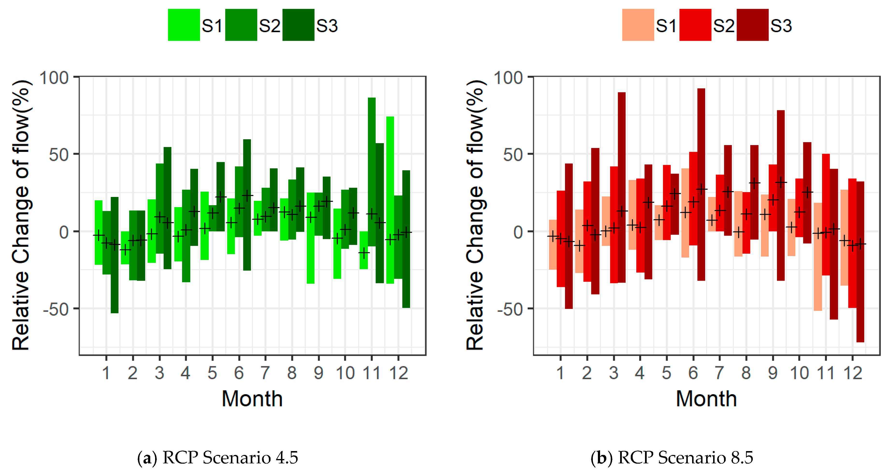
Table 10 and Figure 8 show the relative change of the 30-year average monthly flow for the future periods. In RCP 4.5, in S3 (2071–2099), the flow was expected to show a large increase in May, June, and September and the largest decrease in January. In RCP 8.5, the flow increased most from May to October (summer and autumn), and decreased significantly from December and January (winter). Figure 8 shows that the variability in June, November, December, and January increased as S3 approached. As mentioned in the seasonal flow characteristics, the relative change in the monthly flow also represented the possibility of extreme rainfall and drought in summer (June to October) and winter (December to January).
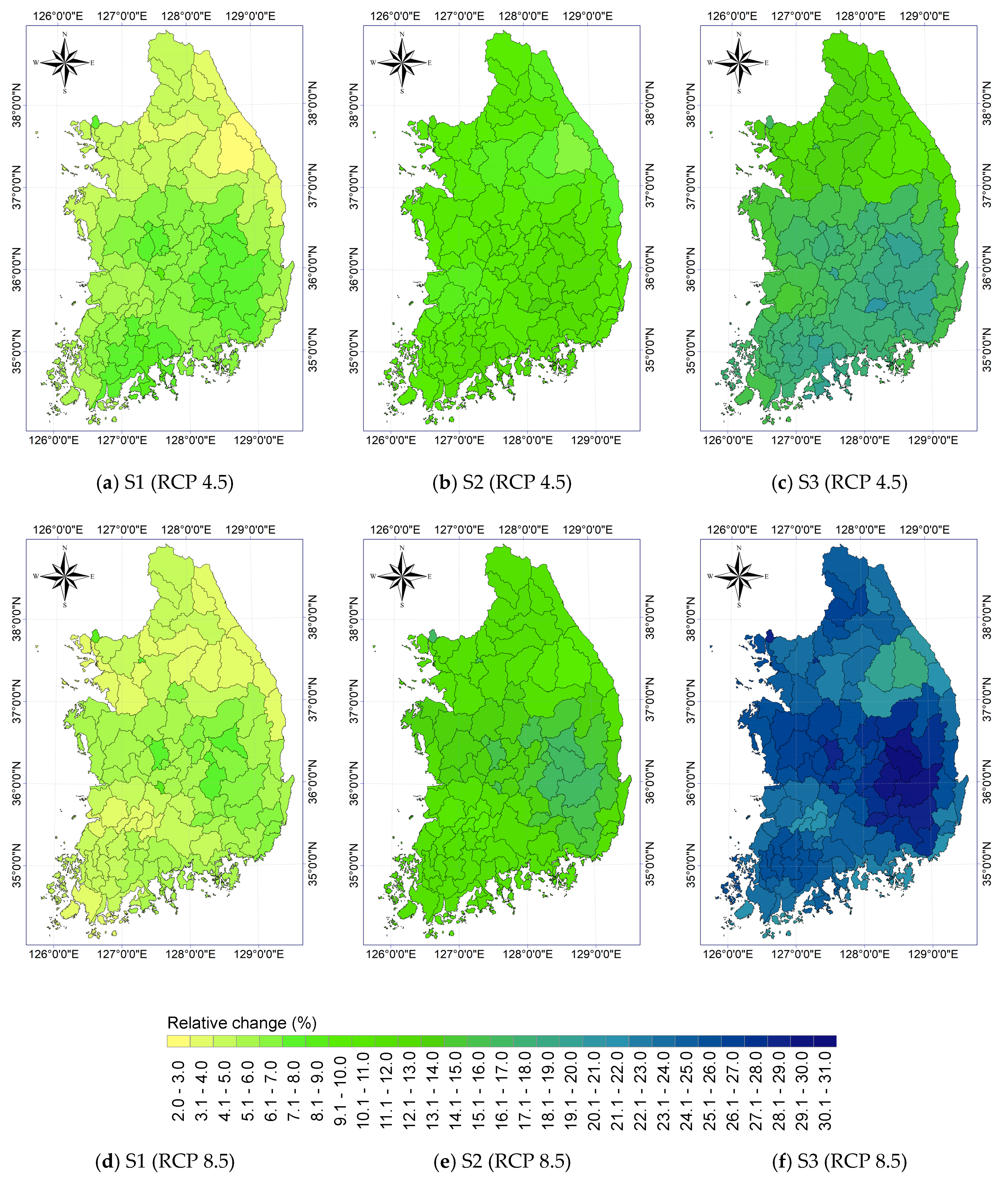
3.2.4. Relative Change Analysis of Future Flow for 109 Mid-Size Watersheds over South Korea
Figure 9 illustrates the relative change of future flow for 109 mid-size watersheds. Overall, it tended to increase as S3 approached. In RCP 4.5 and 8.5, in S3 (2071–2099), the flow was expected to show a significant increase in the southern and southeastern regions. It was analyzed that it was similar to the spatial pattern of the relative change of precipitation. The southeastern region is the Nakdong River basin, one of South Korea’s main rivers. The flood risk in the Nakdong River basin is expected to increase in the future. Therefore, it is considered that countermeasures against floods should be applied first to the Nakdong River basin.
4. Conclusions
This study evaluated the impact of climate change on streamflow in South Korea using downscaled climate change data from 13 GCMs and the HSPF model. The HSPF model was calibrated and validated for six dams with daily streamflow data. Optimized parameters for six dams were employed to perform parameter localization for the remaining mid-size watersheds. The simulation periods were divided into four: S0 (reference: 1976–2005), S1 (near future: 2011–2040), S2 (mid–century: 2041–2070), and S3 (distant future: 2071–2099). For future periods, RCP scenarios 4.5 and 8.5 were used for streamflow projection. The temporal resolution of the future long-term streamflow produced in this study was daily data, and the spatial resolution was 109 mid-size watersheds in South Korea. Finally, according to 13 GCMs, streamflow was analyzed by combining the year, season, and month in South Korea.
South Korea’s 30-year average annual precipitation for the reference period (S0: 1976–2005) was 1306.8 mm, the temperature was 12.4 °C, the potential evapotranspiration was 1055.6 mm, and the flow was 72,969.4 m³. In the future third period (S3: 2071–2099) for RCP 8.5, the 30-year average annual precipitation was expected to increase to 1540.1 mm, the temperature to 16.5 °C, the potential evapotranspiration to 1187.3 mm, and the flow to 90,826.7 m³. The 30-year average annual precipitation in the future third period (S3: 2071–2099) compared with past values was expected to increase by 11.32% and 17.82% for RCP scenarios 4.5 and 8.5, the temperature was expected to increase by 2.29 °C and 4.07 °C, and the potential evapotranspiration by 6.88% and 12.48%. Streamflow was projected to increase by 15.11% and 24.40% for RCP 4.5 and 8.5, respectively. The relative change of the 30-year average seasonal flow during S3 (2071–2099) for RCP 4.5 was as follows: summer (17.13%) > autumn (15.86%) > spring (14.63%) > winter (−4.47%). For RCP 8.5, summer (28.25%) > autumn (26.09%) > spring (19.37%) > winter (−5.12%). Both RCP 4.5 and 8.5 were projected to show the greatest increase in streamflow in summer and fall and decrease in winter. It was anticipated that difficulties in the stable water supply could occur due to the high variability in winter.
Looking at previous studies, the flow in the near future also increased or decreased depending on the region, but the flow in the distant future showed a remarkable increase. The flow varied depending on the hydrological model and periods, such as wet and dry seasons. During the wet period, the relative change in the flow was significantly higher. It also was analyzed that the increase in peak flow and the shifting of the season cycle could affect agriculture and flood disaster management. Notably, the strong annual peak in the future may have a severe impact on floods. There was a trend of decreasing values in winter runoff [2,3,5]. Streamflow projection in South Korea also tended to increase in summer and decrease in winter. It has been shown that the increase in the flow in the distant future was significant.
In terms of the climate change characteristics by seasons in South Korea, the temperature increased evenly in the four seasons. The potential evapotranspiration in the winter increased considerably, while precipitation in the winter increased slightly, which resulted in a decrease in streamflow in winter. This suggests that droughts may be more severe in the current winter than in the future winters. Moreover, as severe droughts could occur when the streamflow in winter decreases and the rate of increase in spring in S1 is insignificant. For this reason, proactively preparing for spring droughts in the near future is necessary. Precipitation is expected to increase to a maximum in summer, therefore, the monsoon period and rainfall intensity are expected to increase in future. In addition, there is a high possibility of extreme flooding in summer. As S3 approaches, it is thought managing rivers, reservoirs, and dams will become more challenging with guidelines that reflect the current design criteria as a result of the high variability of streamflow according to GCM. Therefore, establishing new guidelines that consider climate change, as well as the variability of streamflow in three future periods, is necessary.
This study was conducted to aid in the establishment of a long-term comprehensive plan for water resources at the national level. The results presented in this study could be used as primary data in establishing national climate change adaptation measures in South Korea. Additional research on five major rivers in South Korea is needed to develop detailed plans for major rivers. More specific plans could be established by analyzing streamflow projection, flow duration curve, and hydrologic indicators of five major rivers.
Author Contributions
J.P. performed overall modeling and wrote the manuscript; E.J. constructed topographical data for model input data and analyze results; I.J. performed the parameter optimization and analyze results; J.C. contributed to establish the methodology of this paper and analyze results. All authors have read and agreed to the published version of the manuscript.
Funding
The APC was funded by the APEC Climate Center.
Acknowledgments
This research was supported by the APEC Climate Center.
Conflicts of Interest
The authors declare no conflict of interest.
References
- Olsson, J.; Arheimer, B.; Borris, M.; Donnelly, C.; Foster, K.; Nikulin, G.; Persson, M.; Perttu, A.M.; Uvo, C.B.; Viklander, M.; et al. Hydrological climate change impact assessment at small and large scales: Key messages from recent progress in Sweden. Climate 2016, 4, 39. [Google Scholar] [CrossRef]
- Masood, M.; Takeuchi, K. Climate change impacts and its implications on future water resource management in the Meghna Basin. Futures 2016, 78–79, 1–18. [Google Scholar] [CrossRef]
- Zhang, H.; Wang, B.; Liu, D.L.; Zhang, M.; Feng, P.; Cheng, L.; Yu, Q.; Eamus, D. Impacts of future climate change on water resource availability of eastern Australia: A case study of the Manning River basin. J. Hydrol. 2019, 573, 49–59. [Google Scholar] [CrossRef]
- Qiu, J.; Shen, Z.; Leng, G.; Xie, H.; Hou, X.; Wei, G. Impacts of climate change on watershed systems and potential adaptation through BMPs in a drinking water source area. J. Hydrol. 2019, 573, 123–135. [Google Scholar] [CrossRef]
- Bae, D.H.; Jung, I.W.; Lettenmaier, D.P. Hydrologic uncertainties in climate change from IPCC AR4 GCM simulations of the Chungju basin, Korea. J. Hydrol. 2011, 401, 90–105. [Google Scholar] [CrossRef]
- Shin, M.J.; Eum, H.I.; Kim, C.S.; Jung, I.W. Alteration of hydrologic indicators for Korean catchments under CMIP5 climate projections. Hydrol. Process. 2016, 30, 4517–4542. [Google Scholar] [CrossRef]
- Zhou, Z.; Ouyang, Y.; Li, Y.; Qiu, Z.; Moran, M. Estimating impact of rainfall change on hydrological processes in Jianfengling rainforest watershed, China using BASINS-HSPF-CAT modeling system. Ecol. Eng. 2017, 105, 87–94. [Google Scholar] [CrossRef]
- Göncü, S.; Albek, E. Modeling climate change effects on streams and reservoirs with HSPF. Water Resour. Manag. 2010, 24, 707–726. [Google Scholar] [CrossRef]
- Albek, M.; Bakır Öğütveren, Ü.B.; Albek, E. Hydrological modeling of Seydi Suyu watershed (Turkey) with HSPF. J. Hydrol. 2004, 285, 260–271. [Google Scholar] [CrossRef]
- Singh, J.; Knapp, H.V.; Arnold, J.G.; Demissie, M. Hydrological modeling of the Iroquois river watershed using HSPF and SWAT. JAWRA J. Am. Water Resour. Assoc. 2005, 41, 343–360. [Google Scholar] [CrossRef]
- Saleh, A.; Du, B. Evaluation of SWAT and HSPF within BASINS program for the upper North Bosque River watershed in central Texas. Trans. ASAE 2004, 47, 1039–1049. [Google Scholar]
- Ackerman, D.; Schiff, K.C.; Weisberg, S.B. Evaluating HSPF in an arid, urbanized watershed. JAWRA J. Am. Water Resour. Assoc. 2005, 41, 477–486. [Google Scholar] [CrossRef]
- Amirhossien, F.; Alireza, F.; Kazem, J.; Mohammadbagher, S. A comparison of ANN and HSPF models for runoff simulation in Balkhichai River Watershed, Iran. Am. J. Clim. Chang. 2015, 04, 203–216. [Google Scholar] [CrossRef] [Green Version]
- Kim, S.R.; Kim, S.M. Evaluation of HSPF model applicability for runoff estimation of 3 sub-watershed in Namgang dam watershed. J. Korean Soc. Water Environ. 2018, 34, 328–338. [Google Scholar]
- Hwang, B.H. An Applicability Estimation of the HSPF Model Considering Watershed Scale. Master’s Thesis, Kyungpook National University, Daegu, Korea, 2010. [Google Scholar]
- Kim, N.W.; Shin, A.H.; Kim, C.G. Comparison of SWAT-K and HSPF for hydrological components Modeling in the Chungju dam watershed. J. Environ. Sci. 2009, 18, 609–619. [Google Scholar]
- Kim, S.M.; Park, S.W. Calibration and validation of HSPF model to estimate the pollutant loads from rural small watershed. J. Korea Water Resour. Assoc. 2004, 37, 643–651. [Google Scholar] [CrossRef]
- Zarriello, P.J.; Parker, G.W.; Armstrong, D.S.; Carlson, C.S. Effects of Water Use and Land Use on Streamflow and Aquatic Habitat in the Sudbury and Assabet River Basins; MA Report 2010–5042; U.S. Geological Survey Scientific Investigations: Reston, VA, USA, 2010; pp. 17–32.
- USEPA. A Tool for Managing Watershed Modeling Time-Series Data (WDMUtil); Version 2.0; User’s Manual, Contract No. 68-C-98-010 Work Assignment No; Office of Water, U.S. EPA: Washington, DC, USA, 2001; pp. 1–41.
- U.S. Geological Survey (USGS). User’s Manual for an Expert System (HSPEXP) for Calibration of the Hydrological Simulation Program-Fortran, Water-Resources Investigations Report 94-4168; Hydrologic Analysis Support Section, United States Geological Survey: Reston, VA, USA, 1994; pp. 1–6.
- Cannon, A.J.; Sobie, S.R.; Murdock, T.Q. Bias correction of GCM precipitation by quantile mapping: How well do methods preserve changes in quantiles and extremes? J. Clim. 2015, 28, 6938–6959. [Google Scholar] [CrossRef]
- Eum, H.-I.; Cannon, A.J. Intercomparison of projected changes in climate extremes for South Korea: Application of trend preserving statistical downscaling methods to the CMIP5 ensemble. Int. J. Climatol. 2017, 37, 3381–3397. [Google Scholar] [CrossRef]
- Hargreaves, G.H.; Samani, Z.A. Reference crop evapotranspiration from temperature. Appl. Eng. Agric. 1985, 1, 96–99. [Google Scholar] [CrossRef]
- Hargreaves, G.H.; Allen, R.G. History and evaluation of Hargreaves evapotranspiration equation. J. Irrig. Drain. Eng. 2003, 129, 53–63. [Google Scholar] [CrossRef]
- Allen, R.G.; Pereira, L.S.; Raes, D.; Smith, M. FAO Irrigation and Drainage Paper No. 56; Food and Agriculture Organization of the United Nations: Rome, Italy, 1998; Volume 97, pp. 41–55. [Google Scholar]
- USEPA. Estimating Hydrology and Hydraulic Parameters for HSPF; Technical Note 6, EPA-823-R00-012; Office of Water, U.S. EPA: Washington, DC, USA, 2000; pp. 8–30.
- Moriasi, D.N.; Gitau, M.W.; Pai, N.; Daggupati, P. Hydrologic and water quality models: Performance measures and evaluation criteria. Trans. ASABE 2015, 58, 1763–1785. [Google Scholar]
- Lee, B.-J.; Jung, I.W.; Bae, D.-H. Parameter regionalization of semi-distributed runoff model using multivariate statistical analysis. J. Korea Water Resour. Assoc. 2009, 42, 149–160. [Google Scholar] [CrossRef]
Figure 1.
Study area and 60 automated synoptic observing system (ASOS) locations. The colored area denotes 109 mid-size watersheds, which are separated by a gray line border. The circle represents the 60 ASOS locations, and the number next to the circle represents ASOS ID.
Figure 1.
Study area and 60 automated synoptic observing system (ASOS) locations. The colored area denotes 109 mid-size watersheds, which are separated by a gray line border. The circle represents the 60 ASOS locations, and the number next to the circle represents ASOS ID.

Figure 2.
HSPF topographical input data.

Figure 3.
Result of the HSPF model calibration and validation over Andong dam watershed.


Figure 4.
Annual (a) precipitation, (b) temperature, (c) potential evapotranspiration, and (d) flow during the reference (1976–2005) and future (2005–2099) periods for RCP scenarios 4.5 and 8.5 in South Korea. The values in this figure were calculated by converting daily data into annual data for 13 GCMs. The solid line denotes the average of 13 GCMs, and shaded areas denote the maximum and minimum values of 13 GCMs.

Figure 5.
Relative change (%, °C) of the 30-year moving average annual precipitation, temperature, potential evapotranspiration, and flow compared with the reference period (1976–2005) for RCP scenarios 4.5 and 8.5 using 13 GCM in South Korea. PEVT denotes the potential evapotranspiration. Values were calculated by first converting the daily flow data into annual flow data. Next, the relative change of 30-year moving average for 13 GCMs was calculated and is shown as a box plot.


Figure 6.
Relative change (%) of the 30-year moving average seasonal flow compared with the reference period (1976–2005) for RCP 4.5 using 13 GCMs in South Korea. The values were calculated by first converting the daily flow data into seasonal flow data. Next, the relative change of the 30-year moving average seasonal flow for 13 GCMs was calculated and is shown as a box plot.

Figure 7.
Relative change (%) of the 30-year moving average seasonal flow compared with the reference period (1976–2005) for RCP 8.5 using 13 GCMs in South Korea. The values were calculated by first converting the daily flow data into seasonal flow data. Next, the relative change of the 30-year moving average seasonal flow for 13 GCMs was calculated and is shown as a box plot.

Figure 8.
Relative change (%) of the 30-year average monthly flow compared with the reference period (1976–2005) for the RCP scenarios 4.5 and 8.5 using 13 GCMs in South Korea. The values in this figure were calculated by first converting daily flow data into monthly flow data. Next, the relative change of the 30-year average monthly flow for 13 GCMs was calculated and is shown as a box plot.

Figure 9.
Relative change (%) of the 30-year average flow for 109 mid-size watersheds compared with the reference period (1976–2005) for the RCP scenarios 4.5 and 8.5 using 13 GCMs in South Korea. The values in this figure were calculated by first converting daily flow data into annual flow data. Next, the relative change of the 30-year average flow for 13 GCMs was calculated.


Table 1.
Coupled Model Intercomparison Project 5 (CMIP5) global climate model (GCM) description in this study: model name, resolution, institution, and available variables.
Table 1.
Coupled Model Intercomparison Project 5 (CMIP5) global climate model (GCM) description in this study: model name, resolution, institution, and available variables.
| No. | GCM Name | Resolution (Degree) | Institution | Available Variable a | |
|---|---|---|---|---|---|
| PRCP (mm) | WSPD (m/s) | ||||
| TMAX (°C) | RHUM (%) | ||||
| TMIN (°C) | RSDS (MJ/m2) | ||||
| 1 | INM-CM4 | 2.000 × 1.500 | Institute for Numerical Mathematics | ○ | ○ |
| 2 | HadGEM2-ES | 1.875 × 1.250 | Met Office Hadley Centre | ○ | ○ |
| 3 | NorESM1-M | 2.500 × 1.895 | Norwegian Climate Centre | ○ | |
| 4 | MRI-CGCM3 | 1.125 × 1.122 | Meteorological Research Institute | ○ | ○ |
| 5 | GFDL-ESM2G | 2.500 × 2.023 | Geophysical Fluid Dynamics Laboratory | ○ | ○ |
| 6 | CNRM-CM5 | 1.406 × 1.401 | Centre National de Recherches Meteorologiques | ○ | ○ |
| 7 | CESM1-BGC | 1.250 × 0.942 | National Center for Atmospheric Research | ○ | |
| 8 | IPSL-CM5A-MR | 2.500 × 1.268 | Institut Pierre-Simon Laplace | ○ | ○ |
| 9 | CMCC-CMS | 1.875 × 1.865 | Centro Euro-Mediterraneo per I Cambiamenti Climatici | ○ | |
| 10 | CMCC-CM | 0.750 × 0.748 | Centro Euro-Mediterraneo per I Cambiamenti Climatici | ○ | |
| 11 | IPSL-CM5A-LR | 3.750 × 1.895 | Institut Pierre-Simon Laplace | ○ | ○ |
| 12 | CanESM2 | 2.813 × 2.791 | Canadian Centre for Climate Modelling and Analysis | ○ | ○ |
| 13 | HadGEM2-AO | 1.875 × 1.250 | Met Office Hadley Centre | ○ | |
a Circle (○) denotes that variables are available in individual GCM.
Table 2.
Six representative dam list for the HSPF model calibration and validation.
| ID | Mid-Size Watershed Code | Mid-Size Watershed Name | Calibration Period | Validation Period |
|---|---|---|---|---|
| 1 | 1204 | Goesan Dam | 1996–2005 | 2006–2016 |
| 2 | 2001 | Andong Dam | 1996–2005 | 2006–2016 |
| 3 | 2202 | Imha Dam | 1999–2005 | 2006–2016 |
| 4 | 2015 | Hapcheon Dam | 1999–2005 | 2006–2016 |
| 5 | 3001 | Yongdam Dam | 2003–2005 | 2006–2016 |
| 6 | 4001 | Seomjin river Dam | 1996–2005 | 2006–2016 |
Table 3.
Parameters related to flow of the HSPF model. This table was derived from the United States Environmental Protection Agency [26].
Table 3.
Parameters related to flow of the HSPF model. This table was derived from the United States Environmental Protection Agency [26].
| Parameter | Description | Units | Ranges of Values | |||
|---|---|---|---|---|---|---|
| Typical | Possible | |||||
| Min | Max | Min | Max | |||
| LZSN | Lower zone nominal storage | inches | 3.0 | 8.0 | 2.0 | 15.0 |
| INFILT | Soil infiltration capacity index | inches/h | 0.01 | 0.25 | 0.001 | 0.50 |
| AGWRC | Ground water recession coefficient | none | 0.92 | 0.99 | 0.85 | 0.999 |
| UZSN | Upper zone nominal storage | inches | 0.1 | 1.0 | 0.05 | 2.0 |
| INTFW | Interflow inflow parameter | none | 1.0 | 3.0 | 1.0 | 10.0 |
| LZETP | Lower zone ET parameter | none | 0.2 | 0.7 | 0.1 | 0.9 |
| DEEPFR | Fraction of groundwater inflow to deep recharge | none | 0.0 | 0.20 | 0.0 | 0.50 |
| IRC | Interflow recession parameter | none | 0.5 | 0.7 | 0.3 | 0.85 |
Table 4.
Performance evaluation criteria for the HSPF model parameter calibration [27].
Table 4.
Performance evaluation criteria for the HSPF model parameter calibration [27].
| Scale | Measure | Output Response | Temporal Scale a | Performance Evaluation Criteria | |||
|---|---|---|---|---|---|---|---|
| Very Good | Good | Satisfactory | Not Satisfactory | ||||
| Watershed scale | R2 | Flow b | D-M-A | 0.85 < R2 ≤ 1 | 0.75 < R2 ≤ 0.85 | 0.60 < R2 ≤ 0.75 | R2 ≤ 0.60 |
| NSE | Flow | D-M-A | 0.80 < NSE ≤ 1 | 0.70 < NSE ≤ 0.80 | 0.50 < NSE ≤ 0.70 | NSE ≤ 0.50 | |
| PBIAS (%) | Flow | D-M-A | PBIAS < ±5 | ±5 ≤ PBIAS ≤ ±10 | ±10 ≤ PBIAS ≤ ±15 | PBIAS ≥ ±15 | |
a D, M, and A denote daily, monthly, and annual temporal scales, respectively; b includes stream flow, surface runoff, base flow, and tile flow, as appropriate, for watershed-and field-scale models.
Table 5.
Result of the HSPF model calibration and validation.
| Period | Statistics | Dam | |||||
|---|---|---|---|---|---|---|---|
| Goesan Dam | Andong Dam | Imha Dam | Hapcheon Dam | Yongdam Dam | Seomjin River Dam | ||
| Calibration | PBIAS (%) | −10.3914 | −8.7788 | −10.1586 | −8.3744 | −16.0404 | −4.7378 |
| R2 | 0.7405 | 0.7479 | 0.7195 | 0.7361 | 0.7634 | 0.6963 | |
| NSE | 0.7292 | 0.7201 | 0.7187 | 0.7165 | 0.6679 | 0.6937 | |
| Validation | PBIAS (%) | 2.2801 | 7.4059 | 6.2297 | 5.1429 | 14.2007 | −13.6201 |
| R2 | 0.7941 | 0.8232 | 0.7260 | 0.6670 | 0.8234 | 0.7882 | |
| NSE | 0.7083 | 0.8181 | 0.6761 | 0.6656 | 0.8201 | 0.7823 | |
Table 6.
Optimal parameters of the HSPF model for six dam watersheds.
| Parameter | Description | Units | Goesan Dam | Andong Dam | Imha Dam | Hapcheon Dam | Yongdam Dam | Seomjin River Dam |
|---|---|---|---|---|---|---|---|---|
| LZSN(Urban) | Lower zone nominal storage | inches | 4.154 | 4.135 | 4.045 | 4.135 | 4.135 | 4.135 |
| LZSN(Forest) | ||||||||
| 4.654 | 4.635 | 4.545 | 4.635 | 4.635 | 4.635 | |||
| LZSN (Wetland) | ||||||||
| 4.154 | 4.135 | 4.045 | 4.135 | 4.135 | 4.135 | |||
| LZSN (Agricultural) | ||||||||
| 4.654 | 4.635 | 4.545 | 4.635 | 4.635 | 4.635 | |||
| 2.154 | 2.135 | 2.045 | 2.135 | 2.135 | 2.135 | |||
| LZSN (Water) | ||||||||
| INFILT | Soil infiltration capacity index | inches/hour | 0.003 | 0.003 | 0.002 | 0.031 | 0.003 | 0.210 |
| AGWRC | Ground water recession coefficient | none | 0.858 | 0.855 | 0.989 | 0.855 | 0.855 | 0.926 |
| UZSN | Upper zone nominal storage | inches | 0.054 | 0.055 | 0.059 | 0.055 | 0.055 | 0.051 |
| INTFW | Interflow inflow parameter | none | 9.560 | 9.914 | 9.900 | 9.914 | 9.914 | 9.940 |
| LZETP | Lower zone ET parameter | none | 0.379 | 0.152 | 0.740 | 0.152 | 0.152 | 0.175 |
| DEEPFR | Fraction of groundwater inflow to deep recharge | none | 0.002 | 0.000 | 0.006 | 0.000 | 0.000 | 0.004 |
| IRC | Interflow recession parameter | none | 0.326 | 0.848 | 0.304 | 0.848 | 0.848 | 0.301 |
Table 7.
The 30-year average annual precipitation, temperature, potential evapotranspiration, and flow during the reference and three future periods for RCP scenarios 4.5 and 8.5 in South Korea. The values in this table were calculated first by converting daily data into annual data and subsequently by calculating the 30-year average annual value of 13 GCMs for each period and the average of 13 GCMs.
| Variables | Scenario | S0 (1976–2005) | S1 (2011–2040) | S2 (2041–2070) | S3 (2071–2099) |
|---|---|---|---|---|---|
| Precipitation (mm) | RCP 4.5 | 1306.8 | 1357.3 | 1405.1 | 1455.0 |
| RCP 8.5 | 1355.0 | 1427.9 | 1540.1 | ||
| Temperature (℃) | RCP 4.5 | 12.4 | 13.3 | 14.2 | 14.7 |
| RCP 8.5 | 13.4 | 14.8 | 16.5 | ||
| Potential Evapotranspiration (mm) | RCP 4.5 | 1055.6 | 1083.8 | 1112.2 | 1128.2 |
| RCP 8.5 | 1086.2 | 1132.3 | 1187.3 | ||
| Flow (m³) | RCP 4.5 | 72,969.4 | 76,920.2 | 80,085.9 | 83,982.0 |
| RCP 8.5 | 76,431.5 | 81,937.2 | 90,826.7 |
Table 8.
Relative change (%, °C) of the 30-year average annual precipitation, temperature, potential evapotranspiration, and flow during three future periods for RCP scenarios 4.5 and 8.5 in South Korea. The values were calculated first by converting daily data into annual data. The relative change of 13 GCMs was subsequently calculated for each period, and the average of 13 GCMs was determined.
| Variables | Scenario | S1 (2011–2040) | S2 (2041–2070) | S3 (2071–2099) |
|---|---|---|---|---|
| Precipitation (%) | RCP 4.5 | 3.85 | 7.51 | 11.32 |
| RCP 8.5 | 3.68 | 9.26 | 17.82 | |
| Temperature (°C) | RCP 4.5 | 0.90 | 1.78 | 2.29 |
| RCP 8.5 | 0.99 | 2.42 | 4.07 | |
| Potential Evapotranspiration (%) | RCP 4.5 | 2.67 | 5.37 | 6.88 |
| RCP 8.5 | 2.90 | 7.27 | 12.48 | |
| Flow (%) | RCP 4.5 | 5.43 | 9.71 | 15.11 |
| RCP 8.5 | 4.74 | 12.26 | 24.40 |
Table 9.
Relative change (%) of the 30-year average seasonal flow during three future periods for RCP scenarios 4.5 and 8.5 in South Korea. The values were calculated by first converting the daily data into seasonal data. Next, the relative change of 30-year average seasonal flow for 13 GCMs was calculated for each period, and the average of the relative change of 13 GCMs was determined.
| Variables | Flow (%) | |||||
|---|---|---|---|---|---|---|
| Seasons | RCP 4.5 | RCP 8.5 | ||||
| S1 (2011–2040) | S2 (2041–2070) | S3 (2071–2099) | S1 (2011–2040) | S2 (2041–2070) | S3 (2071–2099) | |
| Spring | −0.85 | 7.22 | 14.63 | 4.41 | 7.89 | 19.37 |
| Summer | 9.48 | 10.97 | 17.13 | 4.90 | 13.49 | 28.25 |
| Autumn | 3.17 | 12.13 | 15.86 | 7.59 | 15.94 | 26.09 |
| Winter | −7.02 | −5.00 | −4.47 | −6.09 | −2.75 | −5.12 |
Table 10.
Relative change (%) of the 30-year average monthly flow during three future periods for RCP 4.5 and 8.5 in South Korea. The values in this table were calculated by first converting the daily data into monthly data. Next, the relative change of the 30-year average monthly flow for 13 GCMs was calculated for each period, and the average of the relative change for 13 GCMs was determined.
| Scenario | Period | Flow (%) | |||||||||||
|---|---|---|---|---|---|---|---|---|---|---|---|---|---|
| JAN | FEB | MAR | APR | MAY | JUN | JUL | AUG | SEP | OCT | NOV | DEC | ||
| RCP 4.5 | S1 | −2.47 | −11.95 | −1.74 | −3.37 | 1.79 | 5.66 | 7.79 | 12.42 | 9.12 | −4.58 | −13.94 | −5.33 |
| S2 | −7.59 | −6.00 | 9.16 | 0.84 | 11.77 | 14.79 | 9.55 | 10.74 | 16.20 | 1.09 | 11.28 | −2.25 | |
| S3 | −8.70 | −5.80 | 5.48 | 12.79 | 22.16 | 23.09 | 15.15 | 16.34 | 19.27 | 11.95 | 5.52 | −0.59 | |
| RCP 8.5 | S1 | −3.18 | −9.30 | 0.13 | 4.06 | 7.26 | 12.25 | 7.20 | −0.51 | 10.95 | 2.63 | −1.29 | −6.04 |
| S2 | −4.74 | 3.80 | 2.11 | 2.41 | 16.23 | 18.95 | 13.50 | 11.15 | 20.36 | 12.34 | −0.89 | −9.24 | |
| S3 | −6.62 | −2.30 | 13.01 | 18.64 | 24.29 | 27.24 | 25.51 | 31.11 | 31.61 | 25.17 | 1.45 | −8.17 | |
© 2020 by the authors. Licensee MDPI, Basel, Switzerland. This article is an open access article distributed under the terms and conditions of the Creative Commons Attribution (CC BY) license (http://creativecommons.org/licenses/by/4.0/).
Share and Cite
MDPI and ACS Style
Park, J.; Jung, E.; Jung, I.; Cho, J. Does Future Climate Bring Greater Streamflow Simulated by the HSPF Model to South Korea? Water 2020, 12, 1884. https://doi.org/10.3390/w12071884
AMA Style
Park J, Jung E, Jung I, Cho J. Does Future Climate Bring Greater Streamflow Simulated by the HSPF Model to South Korea? Water. 2020; 12(7):1884. https://doi.org/10.3390/w12071884
Chicago/Turabian StylePark, Jihoon, Euntae Jung, Imgook Jung, and Jaepil Cho. 2020. "Does Future Climate Bring Greater Streamflow Simulated by the HSPF Model to South Korea?" Water 12, no. 7: 1884. https://doi.org/10.3390/w12071884
Note that from the first issue of 2016, this journal uses article numbers instead of page numbers. See further details here.