A Rainfall Intensity Data Rescue Initiative for Central Chile Utilizing a Pluviograph Strip Charts Reader (PSCR)

Abstract

To develop intensity-duration-frequency (IDF) curves, it is necessary to calculate annual maximum rainfall intensities for different durations. Traditionally, these intensities have been calculated from the analysis of traces recorded by rain gauges on pluviograph strip charts (PSCs). For many years, these charts have been recorded and analyzed by the personnel who operate and maintain the pluviograph gauges, thus the reliability of the observational analysis depends exclusively on the professional experience of the person performing the analysis. Traditionally, the analyzed PSCs are physically stored in data repository centers. After storing rainfall data on aging paper for many years, the risk of losing rainfall records is very high. Therefore, the conversion of PSC records to digital format is crucial to preserve and improve the historical instrumental data base of these records. We conducted the first “Data Rescue Initiative” (DRI) for central Chile using a pluviograph strip charts reader (PSCR), a tool that uses a scanner-type device combined with digital image processing techniques to estimate maximum rainfall intensities for different durations for each paper band (>80,000 paper bands). On the paper bands, common irregularities associated with excess ink, annotations, or blemishes can affect the scanning process; this system was designed with a semi-automatic module that allows users to edit the detected trace to improve the recognition of the data from each PSC. The PSCR’s semi-automatic characteristics were designed to read many PSCs in a short period of time. The tool also allows for the calculation of rainfall intensities in durations ranging between 15 min to 1 h. This capability improves the value of the data for water infrastructure design, since intense storms of shorter duration often have greater impacts than longer but less intense storms. In this study, the validation of the PSCR against records obtained from observational analysis showed no significant differences between maximum rainfall intensities for durations of 1 h, 6 h, and 24 h.

1. Introduction

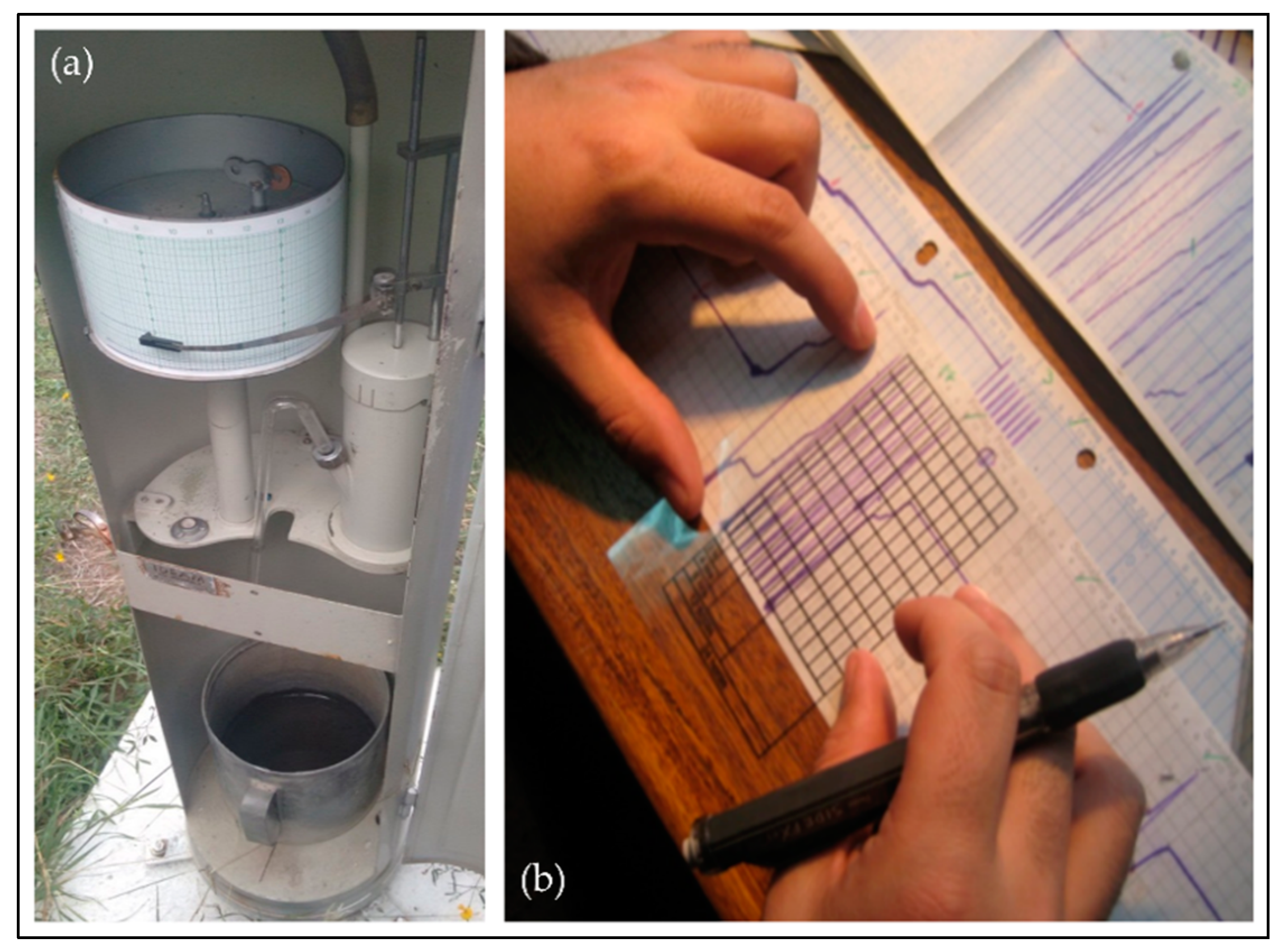
1.1. Pluviograph Strip Charts (PSC) and Observational Rainfall Intensity Reading

Pluviograph rain gauges are devices that continuously measure rainfall intensity. The recorded data have high temporal resolution when compared to pluviometer rain gauges, which only measure daily rainfall accumulation. There are several different types of rain gauges, but the one commonly used in Chile is the float-based pluviograph (see Figure 1a). This device collects rainfall in a bucket containing a lightweight float; as the water level in the container rises, the elevation of the float drives the movement of a pen over a band of paper as it slowly rotates around a cylinder. The dimensions of the collector neck, float, and chamber can be adjusted to accommodate the size of the paper band used to register the rainfall data [1]. Pluviograph gauges can record data for any specific period, but typically the operators replace the bands of paper every week. In Chile, the most common paper used for pluviograph strip charts (PSCs) are 425 mm × 90 mm, with varying color tones and types of paper (Figure 1b).

Analysis of the PSC can determine the maximum rainfall intensity for different durations. This measure, combined with a frequency analysis, can be used to estimate intensity-duration-frequency (IDF) curves, which are considered a fundamental tool for designing hydrologic infrastructure, particularly the dimensions of civil works [2,3]. The reading and the analysis of pluviograph data (see Figure 1b) are traditionally conducted manually by an expert from an official public institution or from a private entity that owns their own instruments. Given the temporal resolution and scale of the typical paper bands (1 week), maximum rainfall intensities can only be determined for durations equal to or longer than 1 h, because a trace length of 2 mm on a band corresponds to approximately 20–30 min of rain. This creates an enormous challenge for the observational analysis of a PSC trace and can result in the introduction and the propagation of large estimation errors by those analyzing the strips. In addition, the feasibility of observational analysis can be limited by the amount of time it takes to process many years of information [4].

1.2. Rescuing Rainfall Data from PSC through Image Processing Techniques

The emergence of digital image processing methods during the last decade has facilitated the implementation of climate data rescue initiatives around the world [5,6,7,8]. These initiatives replace observational/manual PSC reading with (semi) automatic methods that apply algorithms to analyze the image. These methods can significantly reduce estimation errors and processing times as well as increase the potential resolution of the traced rainfall data to durations shorter than 1 h (i.e., as short as 15 min).

One of the first digital image processing algorithms for this process was developed in Italy [9]; a system that extracted rainfall records employed an interactive user interface module to correct inaccurately acquired records. Van Piggelen et al. [10] built on this approach to digitizing PSCs at 321 rain gauges located in the Netherlands. Their analyses showed that, for 30% of the digitized records, semi-automatic processing through a user interface was necessary to correct erroneously acquired traces. These errors were caused mostly by the presence of marks not created by the pluviograph gauge itself but instead by those reading them. For example, rain gauge operators commonly add notes about the current recording period; these handwritten annotations and manual markings introduce inconsistencies and excess ink that challenge the accuracy of digital image processing algorithms. To overcome this issue, Jaklič et al. [4] developed an algorithm for automatic readings and analysis of the pluviograph traces accompanied by a manual adjustment module to improve those traces with poor results. A statistical analysis of their work showed that about 75.9% of the digitized traces were accurate, making the direct validation of rainfall intensities possible. Improvements to the algorithm created by [4] were additionally provided by Sušin and Peer [11], who added an option for manually adjusting results.

Having considered previous international work, we developed a semi-automatic pluviograph strip charts reader (PSCR) to perform a rainfall data rescue initiative (DRI) for central Chile. A high-resolution scanning device was first constructed to scan all available PSC, and digital image-processing algorithms were merged to it to extract and analyze the rainfall trace. A manual adjustment module was also included to correct distortions associated with excess ink, handwritten annotations, or other visual matter that is not part of the original pluviograph trace. All rainfall records rescued from thousands of PSC were stored in a web-based system for the development of IDF curves for central Chile [3,12,13,14,15].

2. Materials and Methods

The architecture of the digital PSCR includes hardware and software components. This architecture, the digital image processing techniques, and the algorithms that were applied to estimate maximum rainfall intensities are described in detail in the following sections. The PSCR’s manual editing module, which can be used to correct the extracted digital trace, is also described.

2.1. Performing Digital Image Processing Techniques on Pluviograph Strip Charts

When reading a PSC manually, the scale marks on the paper—5 mm in a band corresponds to 90–120 min of rain—made it difficult to discern within short durations. The application of digital image processing techniques made it possible to obtain intensities associated with sub-hourly durations between 15 min, 30 min, 45 min, and up to 1 h, 2 h, 4 h, 6 h, 8 h, 12 h, and 24 h, respectively. However, the thickness of the pluviograph trace did not allow for the measurement of maximum rainfall intensities in intervals of less than 5 min. In fact, the validation of durations of less than 5 min revealed large estimation errors. Despite this, the PCSR’s ability to estimate intensity in durations of less than 1 h is a significant improvement in PCS processing central Chile.

2.2. Computing and Network Setup Characteristics

For this PSCR, the minimum computer requirements necessary for image acquisition, digitization, and manipulation of the PSC were 2.2 gigahertz (Ghz) Intel Core i5 processors, 8 Gigabyte (Gb) RAM, and an Intel HD Graphics 4600 graphics processor. The software for interacting with the traces provided by the server was developed with a well-defined and user-friendly interface. The user interface is web-based and was developed using JavaScript and HTML so that the digital image processing could be easily performed on the server without affecting the performance of the local machine. Connecting the computers to the main server provided a storage capacity of 1 terabyte (TB). This was sufficient for storing all the digitized PSCs from the 47 pluviograph gauges analyzed for central Chile, each of which had at least 15 years of historical records totaling more than 80,000 PSCs (see Pizarro et al. [12]). With this system (Figure 2), the server can perform PSC processing at the same time that the user interacts with the image (a process that requires less than a fraction of a second),and the resultant trace on a local computer without the need to interact with the server in any way. In this way, high volumes of PSC images can be processed without connection interruptions, contributing to the operational productivity of the system.

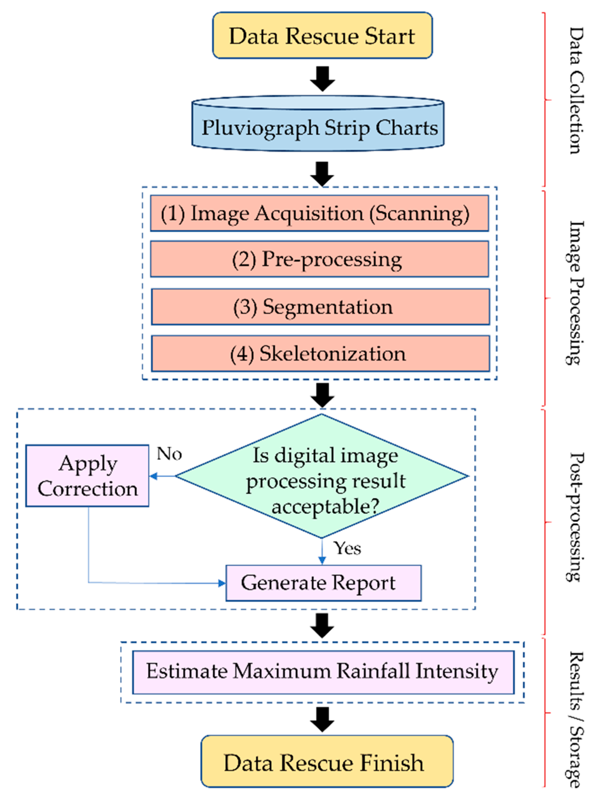
2.3. Data Rescue Initiative and Architecture for Digital Processing of PSC

The data rescue initiative (DRI) conducted for central Chile included four main modules: (1) data collection, (2) image processing, (3) image post-processing, and (4) results and data repository (Figure 3).

Module 1, data collection, was performed for over a year in all available repository centers of the Chilean Meteorological Directorate (DMC in Spanish), the National Directorate of Water Resources of Chile (DGA in Spanish), and the National Company of Electricity (former ENDESA), among others. More than 80,000 PSCs were collected and locally stored to undergo digital image processing.

Module 2, image processing, consisted of four sub-modules: (1) image scanning to convert the analog precipitation signal into a digital signal by scanning a PSC; (2) pre-processing to correct distortions (annotations or marks) present in the acquired image; (3) segmentation to differentiate the target trace from other patterns present in the image; and (4) skeletonization or curve detection, which was the final step used to delineate the target trace by assigning binary values (in pixels) in order to exclude the background of the analyzed image.

Module 3, image post-processing (IPP), was added as an editing tool to improve the performance (if needed) of the detected trace (Figure 3).

With this system, digital traces of 52 weekly PSCs (i.e., 1 year for one pluviograph gauge) can be extracted in about 2 h. The database of digitized traces is evaluated with algorithms to estimate the maximum rainfall intensities associated with different durations (Figure 3). The entire process for DRI involves the collection of PSC, image acquisition or scanning, image processing for digital trace acquisition, manual editing for uncaught errors or distortions, and evaluation for final estimation maximum rainfall intensity. Each one of these stages is obligatory to complete the whole process of DRI. The system for image processing and post-processing resembles those provided by [11,16].

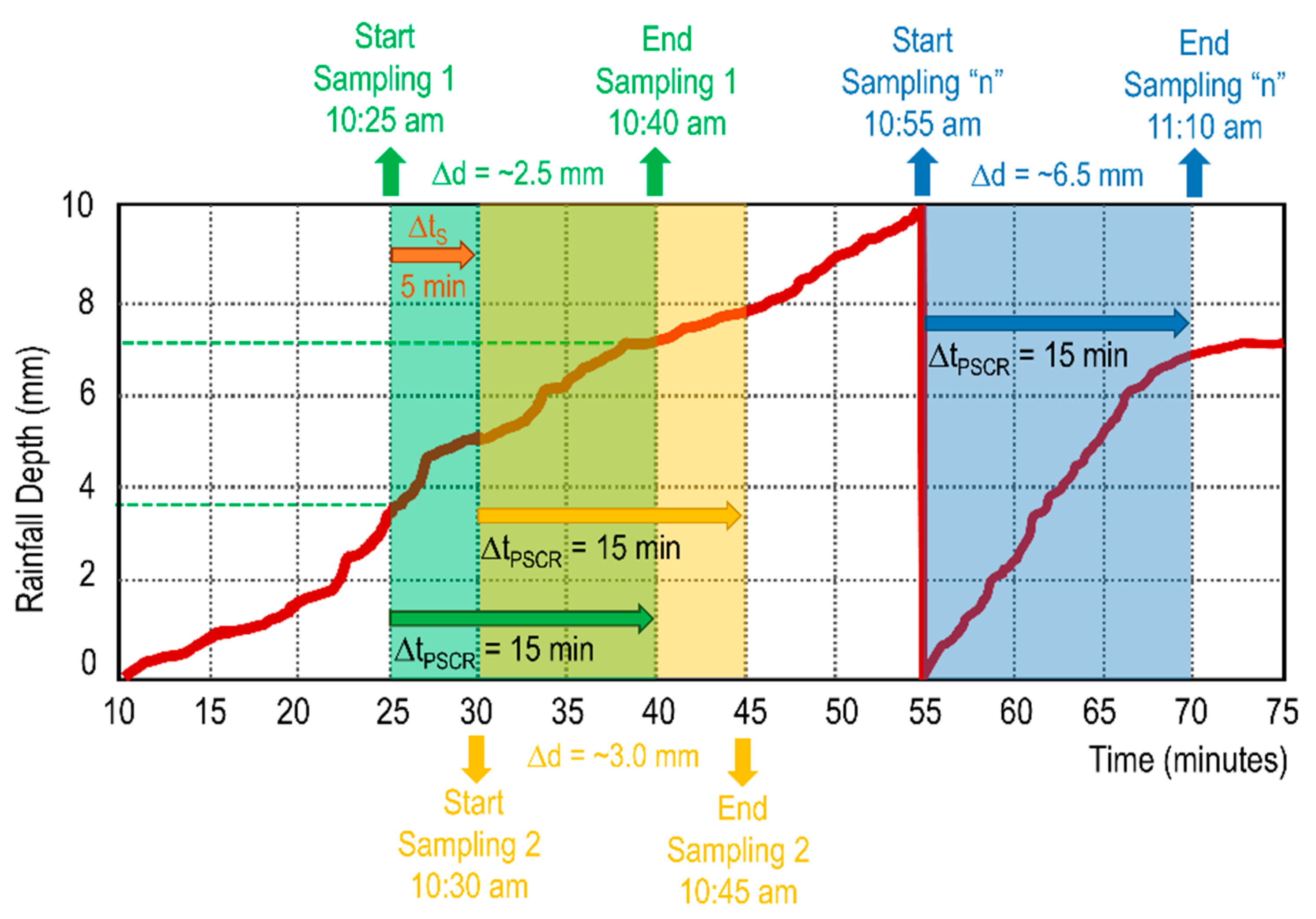
2.4. Sampling Intervals and Estimation of Annual Maximum Rainfall Intensity

In this discussion of rainfall measured by the PSCR process, the rainfall amount is frequently referred to as the rainfall “depth” because the traces on the strip chart are formed by increasing depth of rain the pluviograph bucket. For each processed PSC, the PSCR can generate a report that contains rainfall depths in 15 min periods (Δt_PSCR = 15 min) for a sampling interval (time step) of 5 min (Δt_S = 5 min) (Figure 4). The PCSR’s 5 min sampling interval allows 12 data points for each hour of rainfall event to be generated (i.e., a total of 288 data points per day). Using all the 15 min rainfall data points extracted from the PSC of a single rain gauge, the maximum rainfall intensity (MRI) can be determined for any desired duration.

The maximum rainfall intensity for every year, rain gauge, and for durations larger than 15 min (i.e., 30 min, 45 min, 1 h, 2 h, 4 h, 6 h, 8 h, 12 h, or 24 h) was estimated by constructing a temporal aggregation defined in Equation (1) as:

$$MR{I}_d=\underset{i=d/15,\dots ,n}{\max }\left\{{\displaystyle \sum _{j=i-\frac{d}{15}+1}^{j=i}{h}_j}\right\}$$

(1)

where,

• MRI_d is the annual maximum rainfall intensity (for any rain gauge);
• h_j is the 15 min rainfall depth (mm) at time j;
• i is the time step of the d-minute rainfall. The sum in Equation (1) is the d-minute rainfall depth at time i, aggregated with 15-min records;
• d is the selected rainfall duration (minutes) used for temporal aggregation (accumulation) i.e., 15, 30, 60, 90, 120 min, etc.;
• n is the total number of 15 min rainfall depth data points per year produced by the PSCR.

The expression $\left[\frac{d}{15}+1\right]$ is the index position required to determine the temporal aggregation (accumulation) for the selected duration. For example, to calculate the maximum rainfall intensity for a storm with a duration of 60 min (d = 60), the position of the current 15 min rainfall depth adds three more data points to create an accumulated rainfall depth for 1 h.

2.5. Evaluation and Validation of Rainfall Intensities Estimated from PSCR

To evaluate the performance of the PSCR, a random sampling of pluviograph gauges was conducted, and their historical records were assembled using both the observational reading (traditional method) and the results obtained from the PSCR method. The random sample was limited to only those rain gauges with at least 30 years of rainfall intensity records. The analysis was performed for the durations of 1, 6, and 24 h. The evaluation included three statistical metrics: (1) the mean absolute error (MAE), the relative mean absolute error (RMAE) [4,11,17] and the Mann–Whitney U test [18]. The MAE can be used to estimate the averaged differences (in millimeters) between the traditional method and the PSCR [11]. The RMAE represents the relative error with values ranging between zero and one, where zero means a perfect fit between observational and PSCR readings. In the Mann–Whitney U test, if both the observational reading and the PSCR reading have the same median, then each observational rainfall reading has an equal probability of being greater or smaller than each PSCR rainfall reading. It is also possible that two or more PSCR readings can be equal to the observed rainfall intensity value; therefore, U can be calculated by allocating half of the tie to the observed rainfall intensity records and the other half to the values estimated using the PSCR. This allocation can be performed by using the normal approximation with an adjustment to the standard deviation (see

Table 1. Goodness of fit test parameters.

Goodness of Fit Test	Reference Equation	Parameters
Mann-Whitney U test N < 25	$Z=(N_1\times N_2)+\left(\frac{N_1+N_2+1}{2}\right)-{\displaystyle \sum R_1}$	$H_o$ the distributions R1 and R2 are identical $H_1$ the distributions R1 and R2 are not identical $N_1$ sample size of R1 $N_2$ sample size of R2 $R_1$ sum of ranks of R1 $R_2$ sum of ranks of R2 $n$ number of pairs data to compare $f(i)$ value obtained by traditional method (TM) $\widehat{f}(i)$ Rainfall depth estimated by digital PSCR
Mann-Whitney U test N > 25	$Z=\frac{{\displaystyle \sum R_1}-{\displaystyle \sum R_2}-\left[(N_1-N_2)\times \left(\frac{N_1+N_2+1}{2}\right)\right]}{\sqrt{N_1\times N_2\times \left(\frac{N_1+N_2+1}{3}\right)}}$
Mean Absolute Error (MAE)	$MAE=\frac{1}{n}{\displaystyle \sum _{i=1}^n\left|f(i)-\widehat{f}(i)\right|}$
Relative Mean Absolute Error (RMAE)	$RMAE=\frac{n*MAE}{{\displaystyle \sum _{i=1}^n\left|f(i)-\frac{1}{n}{\displaystyle \sum _{i=1}^{n}f(i)}\right|}}$

). The hypothesis for the test is defined as follows: in the null hypothesis (Ho), the medians of the traditional or manual method (TM) are equal to the median of the digital method (DM); in the alternative hypothesis (Ha), the medians of the traditional method (TM) are different from the median of the digital method (DM). Because the selected rain gauges had an excess of 25 years of records, the Z statistic for Mann–Whitney was calculated for the condition N > 25 as described in Table 1, where Z ~ N (0,1), where Z is said to follow a standard normal distribution. The test used a 95% confidence level (Zα = 1.96), with the comparison criteria established such that, if Z ≤ Zα was accepted, then the (Ho) was accepted, or if Z > Zα was rejected, then the (Ho) was rejected. The application of all these tests allowed us to evaluate the performance of the PSCR through different years and locations (rain gauges).

3. Results and Discussion

The DRI described here allowed us to create the first database of rainfall amounts and maximum rainfall intensities for central Chile (see [12] for reference). The collection and the pre-selection of PSC are intensive activities that can take a significant amount of time and resources within a DRI. However, the conversion of paper-based records to digital records is the most challenging stage of the process (for the final success of a DRI), requiring the development of very specific algorithms for the detection of rainfall traces. For this reason, the focus here is a description of the main features in the PSCR architecture and how accurate maximum rainfall intensities can be obtained from the digital traces; also discussed are the results of an analysis of the validity of the PSCR records using three statistical methods.

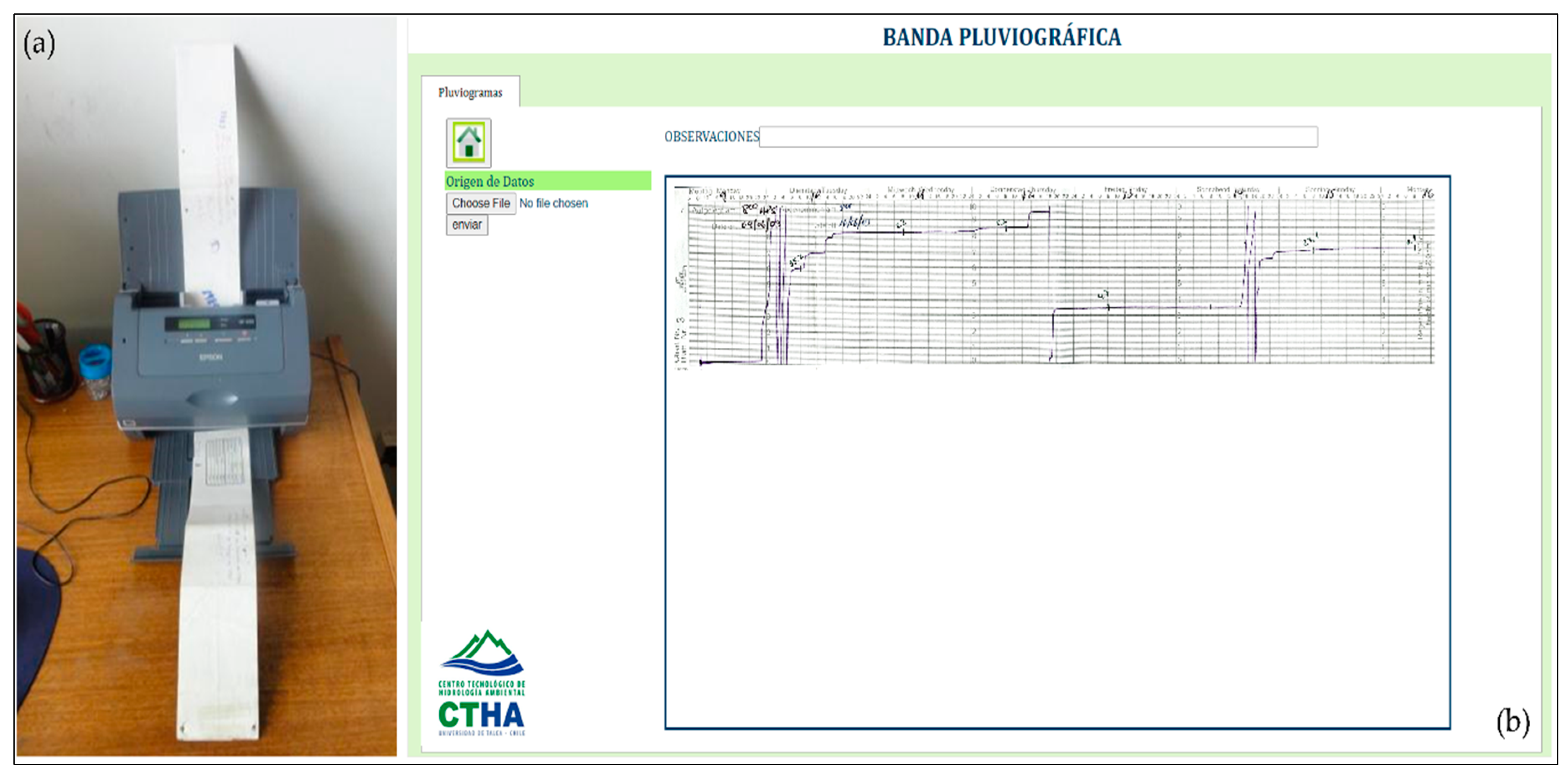
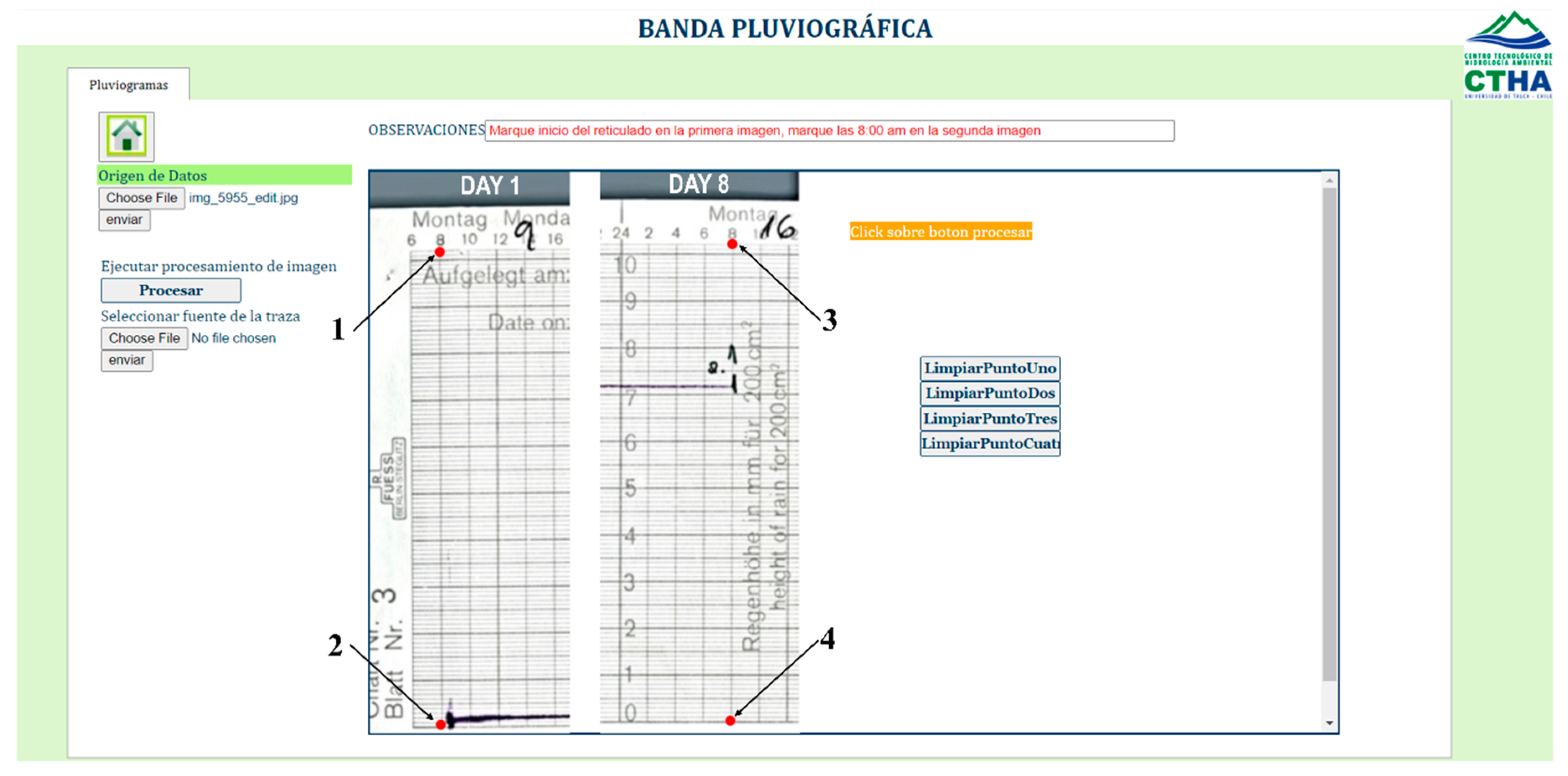
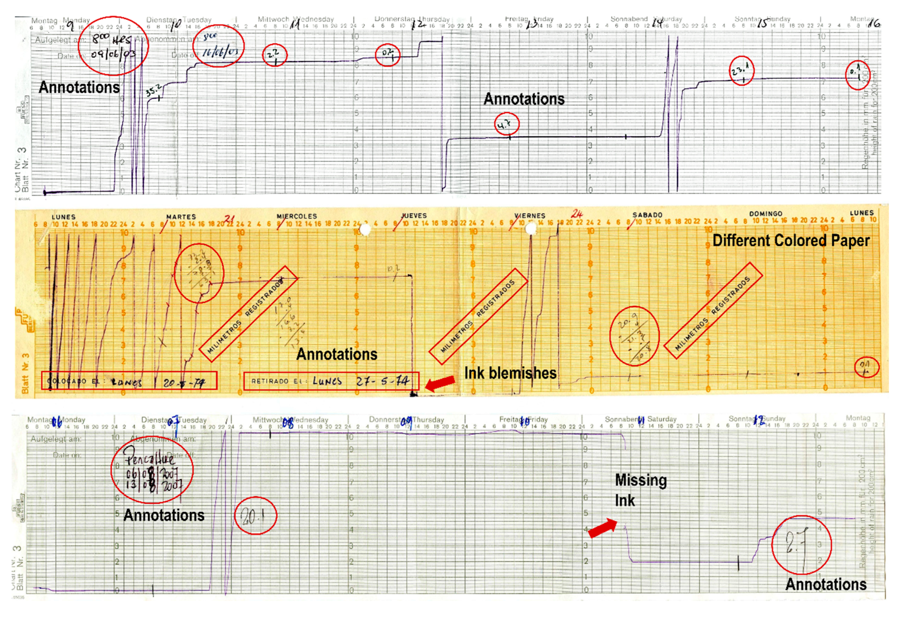
3.1. Image Acquisition

Digital image processing requires a capture device that acquires a specific spectral band, which then generates an electrical signal that is processed by a digitizer. This converts the analogue signal into a digital signal that is then displayed on a computer [19]. Our approach employed a scanner-type device that was used to digitize the PSCs (analogue signals) and convert them into digital images and then send the digital image to a computer for processing. This study used an Epson Workforce Pro GT-S50 scanner with automatic feeder and the ability to scan both sides of the paper, with a capacity of 50 pages per minute (Figure 5). This type of scanner was selected because it did not generate optical distortions and because of its ability to read documents of different dimensions, such as those of the pluviograph strips (425 mm × 90 mm). These features facilitated a rapid scanning process, optimal image quality, and file sizes up to 2 Mb for storage purposes. This scanning device also permits scanning at 300 dpi (dots per inch) to general images of approximately 5019 × 1181 pixels that can be stored in 24 bit color in JPEG format. According to Van Piggelen [10], this image configuration improves trace identification in the segmentation process and reduces the storage space needed for the processed information. For the analysis and the manipulation of the acquired images, a web-based JavaScript graphical user interface was designed (Figure 5b), allowing one or more remote users to execute the image-processing algorithms simultaneously, as described in Section 2.1. The low cost and the simplicity of the PCSR configuration could be a potential solution to implement data rescue initiatives for other countries that have this same problem.

3.2. Image Pre-Processing

The objective of pre-processing is to enhance the clarity of the data found in the image by removing unintentional distortions [19,20]. According to Krig [21], image pre-processing is analogous to the mathematical normalization of a data set, a common step in many feature description methods. There are at least four main families of description methods; among them, one of the most important is the polygon shape descriptors. These can range from image improvements to structural morphology and segmentation techniques. The range of possible pre-processing methods is quite large, and the choice of methods to be used is highly dependent on the data.

In the specific case of the pluviograph band raster, the pre-processing stage that we developed included the user’s participation to define control points on the upper and the lower corners of the digital image that resulted from the pluviograph band. Four control points were established with the purpose of indicating the specific area to which the segmentation algorithm would be applied. Demarcating the useful area is necessary, since most conventional pluviograph gauges record the precipitation intensity on paper strips that vary in terms of printed scales, paper strip dimensions, paper color and texture, and other factors. The scales printed on the paper strip use margins that start at the intersection marked 06:00 h on day 1 and end between 12:00 h and 14:00 h on day 8, although the configuration of the paper strips can vary according to the manufacturer. Most conventional rain gauges in Chile have a weekly clock drum that must be activated each time a paper strip is installed, verifying that the siphon system operates correctly and always starts at the 0.0 mm scale of the paper [22]. Considering the possible distortions on PSC, the manual execution procedure using the graphical user interface consists of marking upper and lower starting points (see numbers 1 and 2 of Figure 6) on the reference mark indicating 06:00 h on the paper strip on day 1 and a set of upper and lower ending points (see numbers 3 and 4 of Figure 6) on the reference mark indicating 08:00 h on day 8. With this approach, homogeneity in the target region was achieved for all digital images, thus the segmentation algorithm could be applied to the target region while excluding areas of the image that were of no interest.

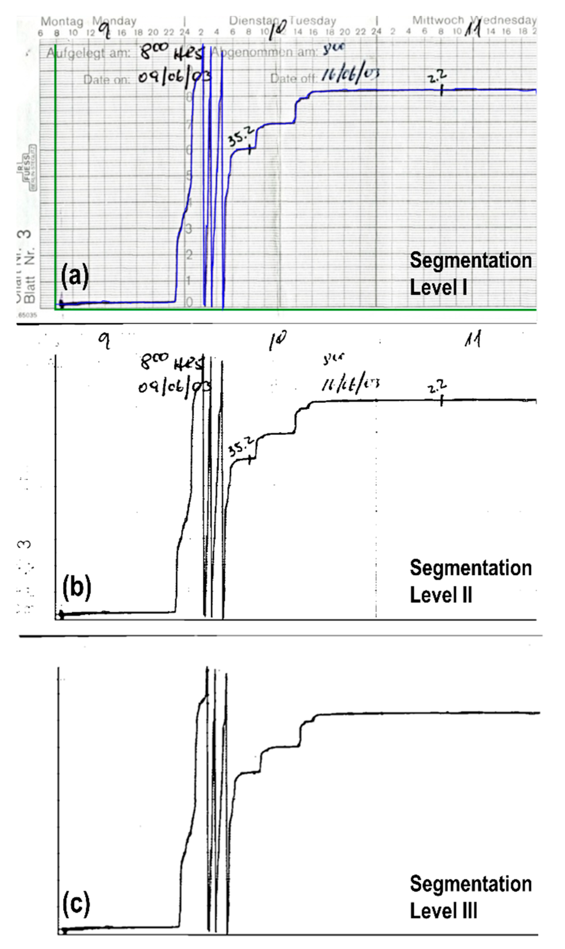
3.3. Image Segmentation

Segmentation is a pre-processing method within the so-called “polygon shape descriptors” family of methods. These methods use structure or texture in the image, rather than a threshold, as the basis for dividing an image into connected polygons, i.e., non-overlapping and significant homogeneous regions corresponding to objects, surfaces, or natural parts of an object [21,23]. For this study, a segmentation technique was developed to distinguish the pluviograph trace in the digital image using a thresholding method [24,25], in which the algorithm is based on similarities (Figure 7). This technique is very efficient for segmenting images with light-colored objects on a dark background (or dark objects on a light background) [25].

One of the problems with the segmentation process is the erroneous classification of band trace pixels. This type of incorrect pixel assignment is frequent, because PSCs generally contain marks that are not generated as part of the measurement process—commonly referred to as “irregularities” in the band. These irregularities include the color of the paper, notes written in ink on the paper, markers with variable widths, and excess ink on the nib that draws the pluviograph trace (Figure 8). This problem is addressed in the next step of the process, skeletonization.

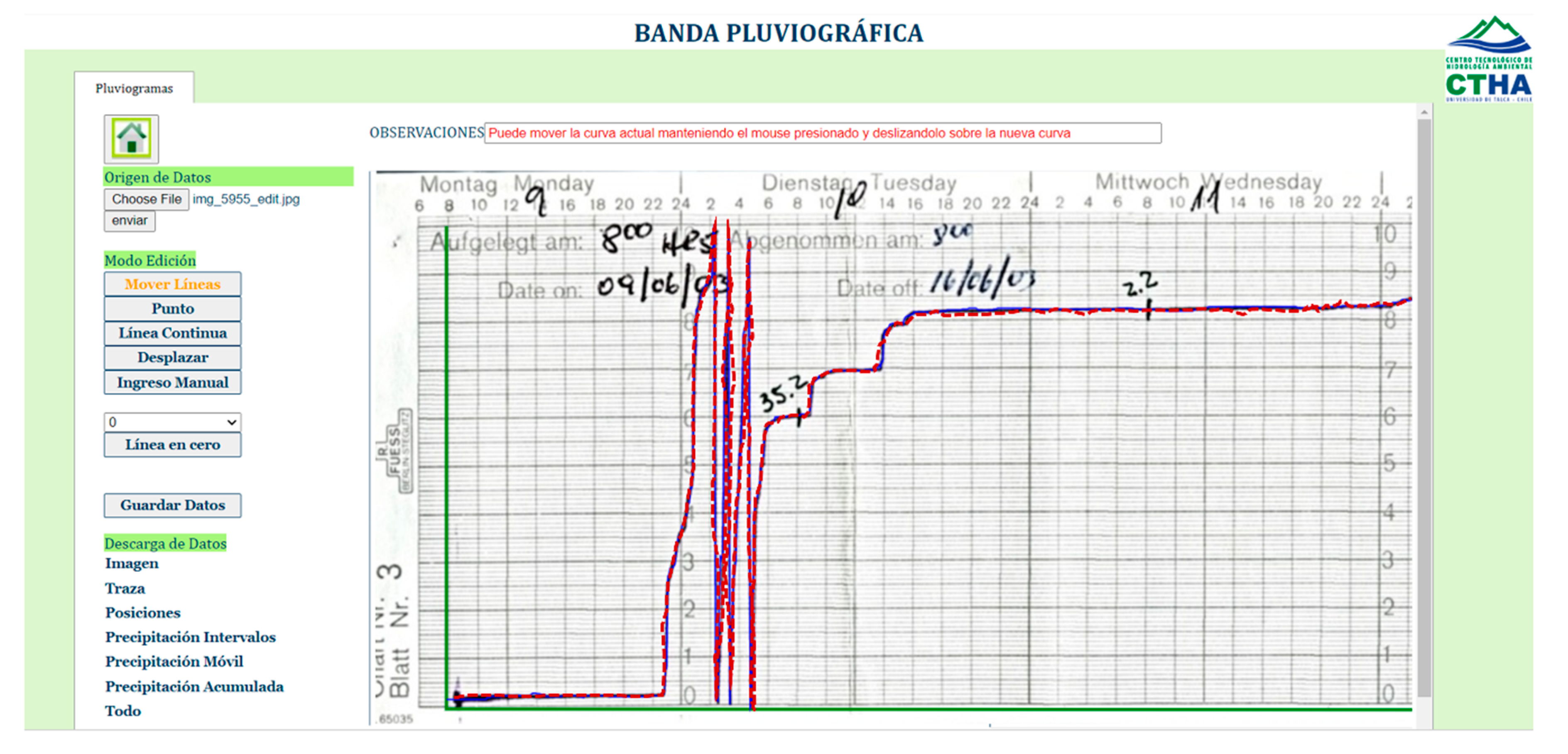
3.4. Image Skeletonization and Rainfall Trace Detection

After the image are segmented into regions as described, the pixels are stored for further processing. A complementary task is the delineation process, since a region can be represented by its boundaries, with information including characteristics such as length, line orientation, and number of concavities at the boundary [19]. In this study, the skeletonization method was developed as described by others [4]. The result of this procedure is a binary image that assigns values of 1 to the pixels that are part of the identified segment and values of 0 to the rest of the identified pixels that correspond to the background of the image. As illustrated in Figure 5, the user can select control points, and these are used by the system as the basis for segmenting and skeletonizing the pluviograph trace. The result is a blue trace, which in ideal conditions follows the path of the pluviograph trace.

At this point, visual analysis is essential to identify errors in the detected patterns that are caused by visual artifacts, such as those shown in Figure 8. In this study, more than 70% of the paper strips had handwritten annotations, excess ink, or other irregularities on the paper. The manual adjustment module permits the elimination of inconsistencies and refines the trace. In the graphical interface environment, the user always has the option to perform manual correction or editing. Once the user has completed the manual editing, the system detects the target trace (Figure 9); the digitization can then be exported to a file with the maximum rainfall intensities for the chosen durations.

3.5. Digital PSCR Report and Maximum Rainfall Intensities

The PSCR generates a report consisting of a package of compressed files containing a JPEG image of the digitized trace and a plain text file (ASCII) with the values of the intensities for durations as low 15 min with displacements of 5 min (Figure 10). The report allows for verification of the control points established for digital processing, the precipitation intervals, and the accumulated precipitation values. Maximum rainfall intensities can be estimated from the report using the algorithm presented in Equation (1).

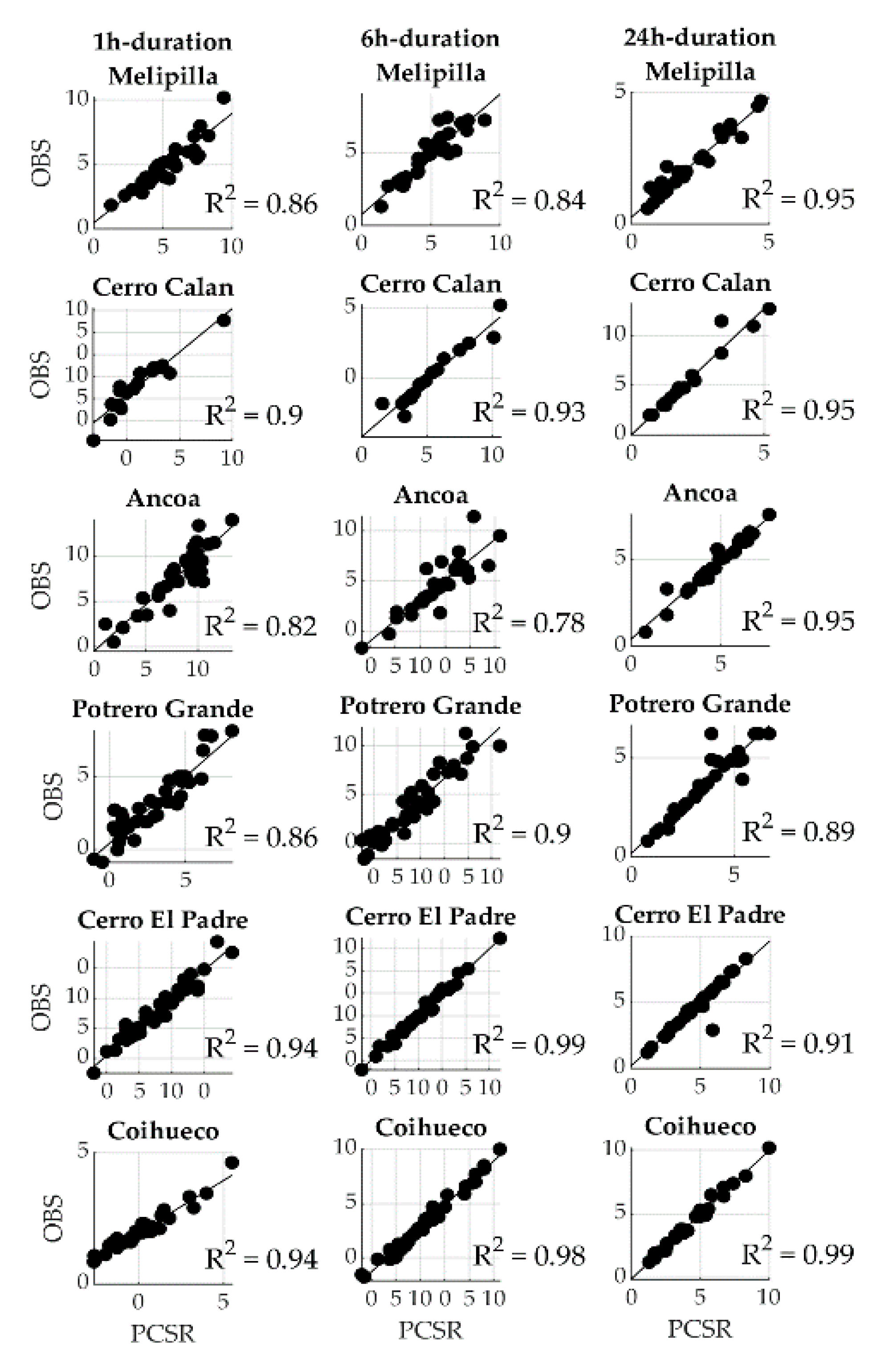
3.6. Evaluating the Performance of DRI through PSCR

The rain gauges in central Chile with the longest records were selected to compare and validate the maximum rainfall intensities estimated using the observational reading method (Figure 1) against those obtained using the digital PSCR method. For all analyzed durations, the statistical tests revealed that MAE did not exceed 2 mm of difference, which is the acceptable error threshold established for rainfall intensity by earlier research [15]. For example, for durations of 1 h, the maximum differences were about 1.5 mm (observed at Embalse Coihueco rain gauge). Similar maximum differences were observed for durations of 1 h and 6 h. For higher durations (i.e., 24 h), the differences between the methods were minimal. Similar validation results were reported by Sušin et al. [11], who found that the errors for high durations (i.e., 24 h) were lower than those errors observed for low durations (i.e., 1 h). It is important to stipulate that the calculated errors can be relative, since the observational reading can be associated with large estimation errors; in particular, low durations are vulnerable to reader error, given that 2 mm of trace on the PSC corresponds to a rain event ranging between 20–30 min. The results of the RMAE agreed with those observed for MAE, because, in general, words are values close to zero, meaning that both manual and digital methods have a similar fit (see

Table 2. Error measures calculated for the rain gauges in central Chile with the longest rainfall intensity records. The error represents the difference between manual readings and digital PSCR readings. DGA: General Directorate of Water Resources.

Station	Period of Records	Number of Years	Source	Lat (S)	Long (W)	Resolution	MAE (mm)	RMAE	Mann-Whitney U
Melipilla						1 h	1.068	0.435	Accepted Ho
	1975–2009	35	DGA	33° 40’ S	71° 11’ W	6 h	0.494	0.372	Accepted Ho
						24 h	0.147	0.160	Accepted Ho
Cerro Calán						1 h	0.728	0.416	Accepted Ho
	1975–2009	35	DGA	33° 23’ S	70° 32’ W	6 h	0.428	0.263	Accepted Ho
						24 h	0.133	0.128	Accepted Ho
Embalse Ancoa						1 h	1.021	0.404	Accepted Ho
	1971–2009	39	DGA	35° 54’ S	71° 17’ W	6 h	0.741	0.373	Accepted Ho
						24 h	0.218	0.190	Accepted Ho
Potrero Grande						1 h	1.400	0.402	Accepted Ho
	1971–2009	39	DGA	35° 12’ S	71° 07’ W	6 h	1.450	0.526	Accepted Ho
						24 h	0.218	0.170	Accepted Ho
Cerro El Padre						1 h	0.840	0.218	Accepted Ho
	1970–2009	40	DGA	37° 46’ S	71° 53’ W	6 h	0.195	0.109	Accepted Ho
						24 h	0.150	0.124	Accepted Ho
Embalse Coihueco						1 h	1.597	0.324	Accepted Ho
	1971–2009	39	DGA	36° 35’ S	71° 47’ W	6 h	0.374	0.159	Accepted Ho
						24 h	0.211	0.134	Accepted Ho

).

From the Mann–Whitney U test, all the null hypotheses (Ho) were accepted, because there were no significant differences between the medians of the observation/manual reading method and the medians of the digital PSCR method at the 95% confidence level (Table 2). These results were based on the maximum rainfall intensity records for 1 h, 6 h, and 24 h durations, respectively (Figure 11). The mechanism for digitally reading pluviograph strips using digital image processing is therefore validated as a tool for obtaining maximum rainfall intensities. This digital method significantly reduces the time needed to analyze rainfall records; it also improves the quality and the reliability of the information used to generate IDF curves, providing accumulation intervals of as little as 15 min (an interval not generally possible with the traditional pluviograph band method).

4. Conclusions

The development of the PSCR has contributed significantly to the success of a rainfall intensity data rescue initiative for central Chile. With this PSCR, a database was compiled of maximum rainfall intensities derived from 47 pluviograph gauges in central Chile. The tool developed in this study produced rainfall intensity estimates that correlated, at the 95% confidence level, with records obtained from the observational or manual analysis. This type of device offers three main advantages and benefits: a simple and low-cost configuration that can be implemented in other countries, a considerable reduction in processing time for PSC, and an improved resolution of maximum rainfall intensities compared with the conventional method, since it was possible to obtain values at sub-hourly durations between 15 min and 1 h.

All the records generated by this data rescue initiative were stored in a Web-based System (WEBSE_IDF) developed for the automatic construction of IDF curves [12]. This tool therefore has contributed to the compilation of historical rainfall storms that can be used to improve water infrastructure design. This first DRI implemented in central Chile provides a high scientific value for the generation of reanalysis climate products [26] and for supporting the global need of meteorological services for rescuing long-term historical records [8]. This is also the first system in Chile capable of producing IDF curves for durations of less than 1 h—an important advance, because extreme rainfall events of short duration have often proved to be more severe and destructive than less intense but longer events. Automating the rainfall data analysis process also makes it easier to collect and manage large volumes of records that have been stored in a physical paper format. In short, this system facilitates collection, storage, transference, and analysis of rainfall intensity records to improve the management and the governance [27] of water related data.

References

1. World Meteorological Organization (WMO No 8). Guide to Instruments and Methods of Observation: Volume I –Measurement of Meteorological Variables; WMO: Geneva, Switzerland, 2018. [Google Scholar]
2. Nhat, L.M.; Tachikawa, Y.; Sayama, T.; Takara, K. A Simple Scaling Charateristics of Rainfall in Time and Space to Derive Intensity Duration Frequency Relationships. Annu. J. Hydraul. Eng. JSCE 2007, 51, 73–78. [Google Scholar] [CrossRef] [Green Version]
3. Pizarro, R.; Valdés, R.; García-Chevesich, P.; Vallejos, C.; Sangüesa, C.; Morales, C.; Balocchi, F.; Abarza, A.; Fuentes, R. Latitudinal Analysis of Rainfall Intensity and Mean Annual Precipitation in Chile. Chil. J. Agric. Res. 2007, 72, 252–261. [Google Scholar] [CrossRef] [Green Version]
4. Jaklič, A.; Šajn, L.; Derganc, G.; Peer, P. Automatic Digitization of Pluviograph Strip Charts. Meteorol. Appl. 2016, 23, 57–64. [Google Scholar] [CrossRef] [Green Version]
5. Brunet, M.; Jones, P. Data Rescue Initiatives: Bringing Historical Climate Data into the 21st Century. Clim. Res. 2011, 47, 29–40. [Google Scholar] [CrossRef]
6. Munang, R.; Nkem, J.N.; Han, Z. Using Data Digitalization to Inform Climate Change Adaptation Policy: Informing the Future Using the Present. Weather Clim. Extrem. 2013, 1, 17–18. [Google Scholar] [CrossRef] [Green Version]
7. Ashcroft, L.; Allan, R.; Bridgman, H.; Gergis, J.; Pudmenzky, C.; Thornton, K. Current Climate Data Rescue Activities in Australia. Adv. Atmos. Sci. 2016, 33, 1323–1324. [Google Scholar] [CrossRef]
8. Brönnimann, S.; Brugnara, Y.; Allan, R.J.; Brunet, M.; Compo, G.P.; Crouthamel, R.I.; Jones, P.D.; Jourdain, S.; Luterbacher, J.; Siegmund, P.; et al. A Roadmap to Climate Data Rescue Services. Geosci. Data J. 2018, 5, 28–39. [Google Scholar] [CrossRef] [Green Version]
9. Deidda, R.; Mascaro, G.; Piga, E.; Querzoli, G. An Automatic System for Rainfall Signal Recognition from Tipping Bucket Gage Strip Charts. J. Hydrol. 2007, 333, 400–412. [Google Scholar] [CrossRef]
10. Van Piggelen, H.E.; Brandsma, T.; Manders, H.; Lichtenauer, J.F. Automatic Curve Extraction for Digitizing Rainfall Strip Charts. J. Atmos. Ocean. Technol. 2011, 28, 891–906. [Google Scholar] [CrossRef] [Green Version]
11. Sušin, N.; Peer, P. Open-Source Tool for Interactive Digitisation of Pluviograph Strip Charts. Weather 2018, 73, 222–226. [Google Scholar] [CrossRef]
12. Pizarro, R.; Ingram, B.; Gonzalez-Leiva, F.; Valdés-Pineda, R.; Sangüesa, C.; Delgado, N.; García-Chevesich, P.; Valdés, J.B. WEBSEIDF: A Web-Based System for the Estimation of IDF Curves in Central Chile. Hydrology 2018, 5, 40. [Google Scholar] [CrossRef] [Green Version]
13. Pizarro, R.; Garcia-Chevesich, P.; Valdes, R.; Dominguez, F.; Hossain, F.; Ffolliott, P.; Olivares, C.; Morales, C.; Balocchi, F.; Bro, P. Inland Water Bodies in Chile Can Locally Increase Rainfall Intensity. J. Hydrol. 2013, 481, 56–63. [Google Scholar] [CrossRef]
14. Pizarro, R.; Abarza Martínez, A.; Balocchi Contreras, F.; Bjarne Bro, P.; Fuentes Lagos, R.; Ingram, B.; Mendoza Mendoza, R.; Morales Calderón, C.; Olivares Santelices, C.; Sangüesa Pool, C.B.; et al. Curvas Intensidad Duración Frecuencia Para Las Regiones Metropolitana, Maule y Biobío. Intensidades Desde 15 Minutos a 24 Horas, PHI-VII/Documento Técnico No. 29; Programa Hidrológico Internacional de UNESCO (PHI) para América Latina y el Caribe: Montevideo, Uruguay, 2013; Available online: http://eias.utalca.cl/Docs/pdf/Publicaciones/libros/IDF_15_24_horas.pdf (accessed on 10 April 2020).
15. Pizarro, R.; Valdés, R.; Abarza, A.; Garcia-Chevesich, P. A Simplified Storm Index Method to Extrapolate Intensity-Duration-Frequency (IDF) Curves for Ungauged Stations in Central Chile. Hydrol. Process. 2015, 29, 641–652. [Google Scholar] [CrossRef]
16. Marchewka, A.; Pasela, R. Extraction of Data from Limnigraf Chart Images. In Image Processing and Communications Challenges 5. Advances in Intelligent Systems and Computing; Ryszard, S.C., Ed.; Springer: Berlin/Heidelberg, Germany, 2014; Volume 233, pp. 263–269. [Google Scholar] [CrossRef]
17. Kononenko, I.; Kukar, M. Machine Learning and Data Mining: Introduction to Principles and Algorithms; Horwood Publishing Limited: West Sussex, UK, 2007. [Google Scholar]
18. Mann, H.B.; Whitney, D.R. On a Test of Whether One of Two Random Variables Is Stochastically Larger than the Other. Ann. Math. Stat. JSTOR 1947, 18, 50–60. [Google Scholar] [CrossRef]
19. Gonzalez, R.C.; Woods, R.E. Digital Image Processing, 3rd ed.; Prentice-Hall, Inc.: Upper Saddle River, NJ, USA, 2008. [Google Scholar]
20. Sonka, M.; Hlavac, V.; Boyle, R. Image Pre-Processing. In Image Processing, Analysis and Machine Vision; Springer US: Boston, MA, USA, 1993; pp. 56–111. [Google Scholar] [CrossRef]
21. Krig, S. Computer Vision Metrics: Survey, Taxonomy, and Analysis; Apress Media LLC: New York, NY, USA, 2014. Available online: https://link.springer.com/book/10.1007/978-1-4302-5930-5#about (accessed on 15 April 2020).
22. Dirección General de Aguas (DGA). Manual Básico Para Instrucción de Hidromensores; DGA, Departamento de Hidrología, Ministerio de Obras Públicas de Chile (MOP): Santiago, Chile, 1991; Available online: https://dga.mop.gob.cl/legistlacionynormas/normas/Reglamentos/proced_hidromensor.pdf (accessed on 15 April 2020).
23. Roy, P.; Goswami, S.; Chakraborty, S.; Azar, A.T.; Dey, N. Image Segmentation Using Rough Set Theory: A Review. Int. J. Rough Sets Data Anal. 2014, 1, 62–74. [Google Scholar] [CrossRef] [Green Version]
24. Haralick, R.M.; Shapiro, L.G. Image Segmentation Techniques. Comput. Vis. Graph. Image Process. 1985, 29, 100–132. [Google Scholar] [CrossRef]
25. Sivakumar, P.; Meenakshi, S. A Review on Image Segmentation Techniques. Int. J. Adv. Res. Comput. Eng. Technol. 2016, 5, 641–647. [Google Scholar]
26. Wilkinson, C.; Brönnimann, S.; Jourdain, S.; Roucaute, E.; Crouthamel, R.; IEDRO Team; Brohan, P.; Valente, A.; Brugnara, Y.; Brunet, M.; et al. Best Practice Guidelines for Climate Data Rescue v1, of the Copernicus Climate Change Service Data Rescue Service. [Ref: C3S_DC3S311a_Lot1.3.4.1_2019_v1-contract: 2019/C3S_311a_Lot1_Met Office/SC2], Technical Report. 2019. Available online: https://climate.copernicus.eu/sites/default/files/2020-02/BestPracticeGuidelines_ClimateDataRescue_0.pdf (accessed on 26 June 2020).
27. Valdés-Pineda, R.; Pizarro, R.; García-Chevesich, P.; Valdés, J.B.; Olivares, C.; Vera, M.; Balocchi, F.; Pérez, F.; Vallejos, C.; Fuentes, R.; et al. Water Governance in Chile: Availability, Management and Climate Change. J. Hydrol. 2014, 519, 2538–2567. [Google Scholar] [CrossRef]
Figure 1. (a) A typical float-based pluviograph used in Chile; (b) observational procedure to recording rainfall intensities.
Water 12 01887 g001
Figure 2. Main components of the pluviograph strip chart reader (PSCR).
Water 12 01887 g002
Figure 3. The flowchart for data rescue initiative (DRI) and the architecture for obtaining maximum rainfall intensities from digital image processing of PSCs.
Water 12 01887 g003
Figure 4. An exaggerated example of the reading process performed by PSCR to obtain maximum rainfall intensities. The rainfall depths (heights) estimated by the PSCR are calculated using an accumulation interval of 15 min (∆tPSCR). The selected sampling interval (time step) for the calculation of maximum rainfall intensities is 5 min (∆tS).
Water 12 01887 g004
Figure 5. The equipment for digitization of pluviograph bands includes (a) a digitizer Epson Workforce Pro GT-S50 and (b) a graphical interface to process acquired images to digitizer.
Water 12 01887 g005
Figure 6. Control points for selecting the target region or area of interest (AOI).
Water 12 01887 g006
Figure 7. The segmentation process: (a) original image from PSC; (b) and (c) segmented image for two different levels of segmentation.
Water 12 01887 g007
Figure 8. Common defects and blemishes on pluviograph bands include different colored paper strips, annotations on band trace, missing trace, and excessive ink blemishes, among many others.
Water 12 01887 g008
Figure 9. Report of digital image after trace detection, and post-editing the pluviograph band trace (red trace).
Water 12 01887 g009
Figure 10. Final file report exported in zipped format and generated output files.
Water 12 01887 g010
Figure 11. Scatter plots showing manual (observed) versus digital PSCR readings for different durations (1, 6, and 24 h). The rows represent different pluviograph gauges, and the columns represent storm durations of 1 h, 6 h, and 24 h.
Water 12 01887 g011