Forest Inventory and Diversity Attribute Modelling Using Structural and Intensity Metrics from Multi-Spectral Airborne Laser Scanning Data

Abstract

Airborne laser scanning (ALS) systems tuned to the near-infrared (NIR; 1064 nm) wavelength have become the best available data source for characterizing vegetation structure. Proliferation of multi-spectral ALS (M-ALS) data with lasers tuned at two additional wavelengths (commonly 532 nm; green, and 1550 nm; short-wave infrared (SWIR)) has promoted interest in the benefit of additional wavelengths for forest inventory modelling. In this study, structural and intensity based M-ALS metrics were derived from wavelengths independently and combined to assess their value for modelling forest inventory attributes (Lorey’s height (HL), gross volume (V), and basal area (BA)) and overstorey species diversity (Shannon index (H), Simpson index (D), and species richness (R)) in a diverse mixed-wood forest in Ontario, Canada. The area-based approach (ABA) to forest attribute modelling was used, where structural- and intensity-based metrics were calculated and used as inputs for random forest models. Structural metrics from the SWIR channel (SWIR_struc) were found to be the most accurate for H and R (%RMSE = 14.3 and 14.9), and NIR_struc were most accurate for V (%RMSE = 20.4). The addition of intensity metrics marginally increased the accuracy of HL models for SWIR and combined channels (%RMSE = 7.5). Additionally, a multi-resolution (0.5, 1, 2 m) voxel analysis was performed, where intensity data were used to calculate a suite of spectral indices. Plot-level summaries of spectral indices from each voxel resolution alone, as well as combined with structural metrics from the NIR wavelength, were used as random forest predictors. The addition of structural metrics from the NIR band reduced %RMSE for all models with HL, BA, and V realizing the largest improvements. Intensity metrics were found to be important variables in the 1 m and 2 m voxel models for D and H. Overall, results indicated that structural metrics were the most appropriate. However, the inclusion of intensity metrics, and continued testing of their potential for modelling diversity indices is warranted, given minor improvements when included. Continued analyses using M-ALS intensity metrics and voxel-based indices would help to better understand the value of these data, and their future role in forest management.

1. Introduction

Airborne laser scanning (ALS) is a globally established technology for building enhanced forest inventories (EFIs) and supplementing effective forest management [1,2]. ALS point clouds are most often derived using near-infrared (NIR; most commonly 1064 nm) tuned lasers. Apart from high reflectivity from vegetated surfaces, NIR lasers offer benefits including eye safety and low atmospheric interference [3]. As a result, NIR-tuned ALS systems have become common place, improving the cost-effectiveness of characterizing vegetation structure and generating best available geo-spatial terrain information.

Since the adoption of ALS technologies in forestry, point cloud-derived height data have been used to characterize forest structure. The intensity of return pulses also provides additional and often complementary information about surface materials [4]. In a review on the role of radiometric ALS correction and calibration, Kashani et al. [5] highlighted the interdisciplinary value of intensity data for classifying natural and urban cover surfaces [6]. Intensity data have been shown to improve the separation of typical landcover surfaces such as concrete and vegetation [7], though careful attention to intensity correction and calibration methods is a prerequisite [8]. The lack of a calibrated intensity response makes the development of models that utilize intensity limited, as they are unable to be reliably transferred between ALS acquisitions and across different sensors and locations.

The desire to amalgamate structural descriptions from ALS and spectral characterizations from multi-spectral imagery has been met with the development and testing of multi-spectral ALS (M-ALS) [9,10,11,12], and the experimental use of hyperspectral ALS systems [13,14,15,16,17]. These systems use multiple laser scanners at varying wavelengths, designed to be sensitive to both the structural assemblage, and spectral response of vegetation from the top of the canopy through to the ground.

A potential benefit of M-ALS intensity data when compared to that from single-wavelength ALS (S-ALS) is that intensity from multiple wavelengths may improve the capacity for applications such as health and species-based forest inventory information. The potential to leverage multiple wavelengths to produce multi-spectral intensity information, as well as to mimic passive optical data by calculating vegetation indices, could be an important step towards improving estimates of vegetation composition and vigor [18]. Passive optical data continue to be indispensable for forest management [19,20,21,22], facilitating the computation of spectral indices such as the Normalized Difference Vegetation Index (NDVI), and providing a means to derive information on land cover, species, and health. These data are, however, limited to capturing information on the top of the canopy, and are unable to detail potentially important information about internal canopy structure and understorey composition [23,24,25], both areas where M-ALS data may prove useful and provide otherwise unattainable data products.

With computation of spectral indices in mind, a critical consideration of M-ALS data is that sensors are made up of laser scanners with diverging beams. Each point within a multi-spectral point cloud, therefore, contains intensity data from a single wavelength only. This contrasts to other three-dimensional remote sensing technologies such as digital aerial photogrammetry (DAP), where all points are attributed with all spectral information derived from overlapping imagery [23,24]. In order to compute vegetation indices using M-ALS point clouds, voxelization approaches can be applied, where all points within a voxel of predetermined size are used to calculate vegetation indices. Okhrimenko et al. [9] found that voxelization of M-ALS wavelengths facilitated the computation of vertical spectral vegetation index profiles using Optech Titan data for stand-level analyses. The aggregation of points to voxels leads to loss in three-dimensional detail, however, also allows for the calculation of spectral indices using M-ALS data. Apart from voxel-based indices, calculations can also be conducted within delineated features such as individual tree extents [26], and at the plot level [10].

Examples of the application of M-ALS data in the literature are growing, with many studies utilizing the Optech Titan M-ALS sensor for land cover and forest inventory analyses [6,10,11,12,26,27,28]. The addition of the 532 nm wavelength is largely driven by the desire to improve sampling of terrain, vegetation, and riparian environments. Canopy attenuation has been more of a challenge with the 532 nm wavelength than the 1064 and 1550 nm wavelengths, likely due to leaf absorption, limiting point densities and vertical distributions within point clouds [3]. The addition of the 1550 nm wavelength has increased water absorption properties and remains eye safe when emitting higher energy pulses.

Land-cover classification studies such as Wang et al. [4] investigated the potential to combine different ALS wavelength data from separate acquisitions, indicating that multiple wavelengths improved the ability to discriminate low vegetation compared to a single wavelength. Hopkinson et al. [3] likewise tested differences between data acquired using a M-ALS sensor and three S-ALS sensors for forest classification. Incorporation of spectral and structural laser return data were found to improve foliage profiling and land surface classifications. Vertical distribution of points, number of ground returns, and characterization of canopy foliage differed among S- and M-ALS datasets, while acquisition configurations such as flight altitude influenced intensity-based characterizations of the canopy [3,29].

Individual tree-based classification studies such as Axelsson et al. [11] have also highlighted the value of M-ALS data. Intensity distributions and features from the upper and outer parts of tree canopies combined with structural characterizations were found to improve classification accuracies. Yu et al. [30] compared S- and M-ALS data to discriminate between three tree species, with findings indicating that models incorporating metrics derived from M-ALS data were most accurate, but were not markedly higher than S-ALS alternatives. Budei et al. [26] corroborated these findings, where the effectiveness of S- and M-ALS for classifying individual trees into forest type, genus, and species was compared. Additional intensity data, and derived vegetation indices such as the NDVI, were found to be influential in improving classification accuracies, especially when species diversity was high (seven classes or more). Application of M-ALS data to predict individual tree attributes such as volume [12] indicated that M-ALS data performed better than S-ALS data, but were not as effective as the combination of optical imagery and S-ALS. The prediction accuracy of above-ground carbon storage using M-ALS was found to be 11% higher than S-ALS in urban trees, and that the combination of spectral and structural data were influential in improving tree detection and delineation outputs [27].

Given the success of land-cover and individual tree-based classifications, there is an opportunity to further assess the potential of these data for area-based approaches (ABA; [31]). The ABA combines geo-located field samples and ALS metrics to create predictive models of inventory attributes. Following model creation, these models can be applied over the entire coverage of ALS acquisitions, providing managers with wall-to-wall coverage of inventory predictions with known errors [1]. Boreal tree species composition predictions using M-ALS data were found to be comparable to those from conventional ALS and optical data combined [28], indicating that intensity values from M-ALS improve tree species discrimination. Comparison of ALS and DAP metrics for ABA inventory modelling indicated that the use of DAP spectral metrics provided no benefit [24]. Further investigations into the benefit of additional wavelengths for structural and spectral characterizations of inventory attributes is warranted, especially given the success of the ABA using traditional S-ALS systems.

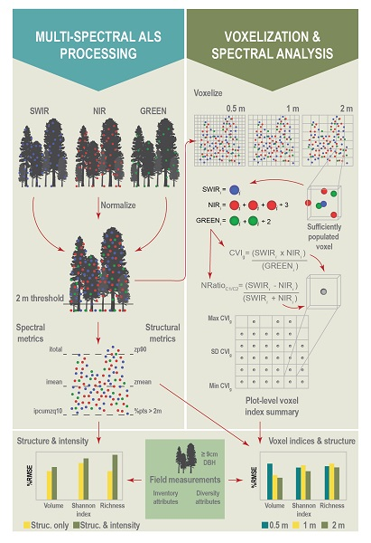
In this study, we assess the potential of M-ALS structural metrics for modelling conventional forest inventory attributes, as well as determine the added benefit of intensity information for estimating a number of plot-level forest stand attributes, including species richness, a variable commonly estimated poorly from S-ALS. To do so, we develop predictive models under two scenarios. First, structural and intensity metrics from each M-ALS wavelength, and all wavelengths combined, were generated and used as predictor variables within random forest (RF) models. Second, the point clouds were voxelized, and a variety of spectral indices calculated, for each voxel. Computed indices were summarized to the plot level and used as RF predictors. By comparing the two approaches, we investigate the potential benefit of M-ALS vegetation indices for improving forest attribute model predictions using an ABA, as well as better understand the potential value of voxel-based vegetation indices derived from M-ALS intensity data.

2. Methods

2.1. Study Site

This research took place at the Petawawa Research Forest (PRF; 45°57′ N, 77°34′ W) near Chalk River, Ontario, Canada (Figure 1). Established in 1918, the PRF has been the location for numerous short- and long-term research initiatives, leading to variation in stand structures and compositions [32]. The PRF is situated at approximately 350 m above sea level and is composed of both planted and naturally regenerating stands. The forest is naturally diverse with respect to tree species, with overstorey conifer species including jack (Pinus banksiana Lamb.), white (Pinus strobus L.), and red pine (Pinus resinosa Ait.), and eastern hemlock (Tsuga canadensis L.), while deciduous species include trembling aspen (Populus tremuloides Michx), sugar (Acer saccharum Marsh) and red maple (Acer rubrum L.), red oak (Quercus rubra L.), and white birch (Betula papirifera Marsh.).

2.2. Data

2.2.1. Field Data

A total of 84 circular 1000 m² field plots were selected from previously established plots [33] that were representative of predominant provincial forest types and basal area conditions [34]. Measurements occurred in the summer of 2016 and 2017, where species and diameter at breast height (DBH) were measured for all trees with DBH ≥ 9 cm (

Table 1. Summary statistics for forest inventory and diversity index attributes. N = 84.

Attribute	Min	Mean	Max	SD
Nha	50	886.1	2420	429.1
HL (m)	6.6	19.9	33.6	6.5
V (m3/ha)	20.6	236.5	734.6	144.4
BA (m2/ha)	5.1	27	54.5	10.9
D	0	0.6	0.8	0.2
H	0	1.3	2.2	0.5
R	1	7	12	3

). A representative subset of field measured trees from each plot were selected based on species and diameter class to create species-specific DBH to height regression models. Models were then applied to trees where only species and diameter were measured [35]. Tree-level attributes were used to summarize gross volume (V, m³/ha), basal area (BA, m²/ha), Lorey’s height (HL, m), and stem density per hectare (Nha) at the plot level. Plot centers were geo-referenced using a SX Blue II-GNSS survey grade GPS unit.

Plot-level diversity indices of overstorey species including the Shannon index, Simpson index, and species richness (species count per plot) were calculated using the following equations:

$$H=-{\displaystyle \sum }_{i=1}^{R}pi ln pi$$

(1)

$$D=1-{\displaystyle \sum }_{i=1}^R{p}_i^2$$

(2)

where H is the Shannon index, D is the Simpson index, R is the species richness, and $pi$ is the proportion of individuals belonging to the $i$th species.

2.2.2. Multi-Spectral Lidar

M-ALS data were acquired on July 20th 2016 using a Teledyne Optech Titan multi-wavelength scanning system during leaf-on conditions. Due to a known temporary scan line intensity banding effect with the Optech Titan sensor [9,29], the number of single and split returns from opposing scan directions were compared for individual M-ALS channels (Figure 2). Comparisons demonstrated that the number of recorded returns from right-traveling (relative to flight path) scan lines were 20.3% and 24.5% higher than those from left-traveling scan lines for single and split returns, respectively. Points from left-traveling scan lines were, therefore, marked as compromised and omitted from analysis [9]. This phenomenon can occur due to a misalignment between returning pulses and the scanner mirror, leading to a reduction in energy passing through the optical path [36]. The removal of the compromised scanlines resulted in the loss of point cloud density for all M-ALS channels. Specifications for the M-ALS data for the full and reduced data are in

Table 2. M-ALS (Optech Titan) acquisition specifications. SWIR–short-wave infrared; NIR–near-infrared; AGL–above ground level.

Parameter	Value	Mean Pulse Density Full Dataset (Points m−2)	Mean Pulse Density Reduced Dataset (Points m−2)	Beam Divergence (mrad)	Footprint Diameter (m)
Wavelength	SWIR (1550 nm)	9.6	5.8	0.35	0.38
	NIR (1064 nm)	10.0	6.2	0.35	0.38
	GREEN (532 nm)	4.1	2.8	0.70	0.77
Flying altitude	1100 m AGL
Pulse repetition rate	375 kHz
Scanning frequency	40 Hz
Scan half angle	20°
Flight line overlap	50%

.

2.2.3. M-ALS Data Processing

The methodology for this study is summarized in Figure 3. Structural and intensity metrics were derived from each M-ALS point cloud following height normalization using ground returns from the NIR channel. Metrics were used to generate predictive models using structural metrics only, as well as the combination of structural and intensity metrics for each M-ALS channels, and all channels combined. Height-normalized M-ALS point clouds were then voxelized at 0.5, 1, and 2 m resolutions, within which mean intensities for each channel were computed. Voxels containing at least 1 point from each M-ALS channel - referred to herein as sufficiently populated - were isolated to compute a suite of voxel-level vegetation indices for each voxel resolution. Plot-level summaries of voxel indices were used as predictor variables for RF models. To analyze the benefit of the additional multi-spectral information collected, structural metrics were calculated using the NIR band only (NIR_struc), akin to a traditional S-ALS data acquisition. NIR_struc were combined with voxel indices to compare their effectiveness. Models incorporating spectral only, structural only, and the combination of metrics were generated to enable comparison between predictor pools and voxel resolutions. Following modelling, the distribution of M-ALS points within voxels were analyzed to understand factors limiting spectral index computation, while spectral metrics produced for each voxel resolution were analyzed to outline differences or trends in computation and consistency.

Following height normalization using ground returns from the NIR channel, ALS data were co-located with field plot locations, and structural metrics were computed for each M-ALS wavelength using the lidR package in R [37]. Computed structural (SWIR_struc, NIR_struc, and GREEN_struc) and intensity (SWIR_int, NIR_int, and GREEN_int) metrics are listed in

Table 3. List of structural metrics calculated for M-ALS point clouds.

Structural Metrics	Description
zmax	maximum height
zmean	mean height
zsd	standard deviation
zskew	skewness
zkurt	kurtosis
zp5, zp10, …, zp95	5th–95th percentile of height
zpcum1, zpcum2, …, zpcum9	cumulative percentage of returns within vertical strata (Woods et al., 2008; Tompalski et al., 2019).
prop_>_threshold2	proportion of points above 2 m
prop_>_threshold5	proportion of points above 5 m
prop_>_mean	proportion of points above mean
prop_>_median	proportion of points above median
prop_d_05, prop_d_2, … prop_d_15	density of points within vertical strata (e.g., prop_d_15 is the proportion of points from ground to 15 m)

and

Table 4. List of intensity metrics calculated for M-ALS point clouds.

Intensity Metrics	Description
itot	total intensity
imax	maximum intensity
imean	mean intensity
isd	standard deviation of intensity
iskew	skewness of intensity
ikurt	kurtosis of intensity
ipcumzq10–ipcumzq90	cumulative proportion of intensity within vertical strata

respectively.

In order to undertake plot-level comparisons, normalized point clouds were voxelized at 0.5, 1, and 2 m resolutions. Voxels containing at least 1 point from each M-ALS channel were considered sufficiently populated and were included for spectral index calculations. The total number of sufficiently populated voxels, the number of voxels containing only points from the NIR and SWIR channels, and voxels containing points from M-ALS channels individually were separately tallied to understand the distribution of points within respective voxel resolutions.

Using only sufficiently populated voxels, the mean intensity of each wavelength was computed and used in the following equations such that indices were calculated for all channel pairings:

$$NRati{o}_{C1/C2}=\frac{(C{1}_{mean}-C{2}_{mean}) }{(C{1}_{mean}+C{2}_{mean})}$$

(3)

$$Sum=C{1}_{mean}+C{2}_{mean}+C{3}_{mean}$$

(4)

$$Rati{o}_{C1/C2}=\frac{C{1}_{mean}}{C{2}_{mean}}$$

(5)

$$CV{I}_{C1}=\frac{(C{2}_{mean}\ast C{3}_{mean})}{C{1}_{mean}^2}$$

(6)

where $NRatio$ is a normalized difference ratio between channels, $CVI$ is the chlorophyll vegetation index [38] adapted to use SWIR and NIR channels, and $C{1}_{mean}$, $C{2}_{mean}$, and $C{3}_{mean}$ are the mean intensity of SWIR, NIR, and GREEN M-ALS channels within voxels. Voxel-level vegetation indices were then summarized to the plot level and used as predictor variables for RF modelling (

Table 5. List of metrics calculated using plot-level summaries of voxel vegetation indices, where SI is the computed spectral index.

Voxel Index Summaries	Description
SI_Mean	Mean of voxel index
SI_Sd	Standard deviation of voxel index
SI_P5, SI_P10, …, SI_P95	Voxel index percentiles
SI_L10, SI_L20, …, SI_L100	Average voxel index within increasing 10% height layers.
SI_above_Z_P5, SI_above_Z_P10, …, SI_above_Z_P95,	Voxel index value above specified height thresholds
SI_zmax_mean	Average voxel index value of the uppermost populated voxels

).

2.3. Random Forest Modelling

Prior to modelling, Pearson’s correlation coefficient (r) was calculated for structural and intensity metrics, as well as plot-level voxel index summaries. If metrics had a r > 0.9, a single metric was randomly retained, while other metrics were removed from predictor pools. Metrics were then centered and scaled to a mean of 0 and standard deviation of 1 to standardize all data and improve model interpretability [39,40]. Plot-level models were generated for each key forest inventory attribute (V, BA, HL) and diversity index (H, D, R) for overstorey species using conditional RF within the caret package in R [41]. Conditional RF were used to reliably quantify the importance of individual metrics within models. Conditional permutation importance can reliably reflect the true impact of predictor variables, in this case structural and intensity metrics, by accounting for correlations [42], thus allowing for more meaningful variable selection and interpretation. Models were all trained using leave-one-out cross-validation and were tuned using the cforest_unbiased function, which returns settings suggested for the construction of unbiased random forests [43].

Four separate modelling strategies were tested:

• Structural metrics from each M-ALS wavelength independently and combined.
• Structural and intensity metrics from each M-ALS wavelength independently and combined.
• Voxelized spectral indices at 0.5, 1, and 2 m resolutions only.
• Voxelized spectral indices at 0.5, 1, and 2 m resolutions combined with structural metrics from the NIR wavelength.

Models combining structural and intensity metrics and voxelized indices were assessed to inform on the added benefit of including both metric types in a single model, and to determine whether a particular voxel resolution outperformed others. All models were validated using leave-one-out cross-validation, and conditional variable importance measures were calculated to understand and compare the benefit of spectral and structural metrics within models [24,42]. Variable importance measures from final models were compared and the most important metrics were identified. Model performance was evaluated based on relative root mean squared error (%RMSE), and relative bias (%bias) using the following equations:

$$\%bias=100\times \frac{\frac{1}{N}{\sum }_{i=1}^N\left({\widehat{y}}_i-y_i\right)}{\overline{y}}$$

(7)

$$\%RMSE=100\times \sqrt{{\displaystyle \sum }_{i=1}^N\frac{{\left({\widehat{y}}_i-y_i\right)}^2}{N}}/\overline{y}$$

(8)

where $N$ is the number of plots, ${\widehat{y}}_i$ are model predicted values of plot $i$, $y_i$ are observed values in plot $i$, and $\overline{y}$ is the mean of observed $y$ values.

Statistical equivalence tests were performed for each model, where observed values were used as a reference [24,44,45]. Tests were performed using the equiv.boot function from the equivalence package in R [46], which bootstraps a regression-based equivalence test for model validation. Statistical equivalence is determined by establishing linear models between observed and predicted values and comparing these values to predetermined regions for slope and intercepts. Slope and intercept tests are performed independently, where statistical equivalency ranges are compared to confidence intervals [46]. The default of ± 25% was used for regions of equivalence following previous studies [24,47,48].

3. Results

3.1. Structural and Intensity Point Cloud Metrics

Our study focused on the potential benefits of point cloud intensity metrics and voxelized indices for estimating forest inventory attributes and overstorey species diversity. Models developed using SWIR_struc were shown to be the most accurate for H (%RMSE = 14.3, %bias = 0.1) and R (%RMSE = 14.9, %bias = 0.3;

Table 6. %RMSE and %bias results for structural only and combination of structure and intensity models derived from the shortwave-infrared (1550 nm) M-ALS wavelength.

SWIR
	Structural + Intensity		Structural Only
Variable	%bias	%RMSE	%bias	%RMSE
HL	−0.3	7.5	−0.1	8.7
V	0.3	21.3	−0.1	21.0
BA	−0.1	14.8	−0.2	14.4
D	0.1	13.3	−0.4	14.6
H	0.4	15.2	0.1	14.3
R	0.7	15.8	0.3	14.9

). Addition of SWIR_int for these models was found to increase %RMSE (Table 6). Both SWIR_{struc and} NIR_struc models for HL had a %RMSE = 8.7 (Table 6,

Table 7. %RMSE and %bias results for structural only and combination of structure and intensity models derived from the near-infrared (1064 nm) M-ALS wavelength.

Nir
	Structural + Intensity		Structural Only
Variable	%bias	%RMSE	%bias	%RMSE
HL	−0.3	7.8	−0.1	8.7
V	−0.2	20.2	0.8	20.4
BA	0.2	13.9	0.2	12.7
D	−0.1	13.4	−0.1	14.3
H	0.5	15.2	0.5	16.3
R	0.8	16.0	0.1	16.8

). GREEN_struc+int models for all attributes were found to show a decrease in %RMSE compared to the structural only models (

Table 8. %RMSE and %bias results for structural only and combination of structure and intensity models derived from the Green (532 nm) M-ALS wavelength.

Green
	Structural + Intensity		Structural Only
Variable	%bias	%RMSE	%bias	%RMSE
HL	−0.2	7.7	0.2	8.9
V	0.1	20.1	1.1	21.1
BA	0.13	12.5	0.4	13.2
D	0.2	13.4	−0.4	14.0
H	−0.1	15.4	0.4	16.4
R	0.5	14.7	0.6	15.4

). Models using Combined_struc+int were found to be the most accurate for V (%RMSE = 19.1, %bias = 0.8;

Table 9. %RMSE and %bias for structural only and combination of structure and intensity models derived from the all M-ALS wavelengths combined.

Combined
	Structural + Intensity		Structural Only
Variable	%bias	%RMSE	%bias	%RMSE
HL	−0.1	7.5	0.2	9.1
V	0.8	19.1	0.7	22.0
BA	0.3	12.2	0.2	12.3
D	0.3	11.5	0.4	14.0
H	0.5	14.8	0.7	16.1
R	0.4	15.9	1.1	15.3

). SWIR_struc+int and Combined_struc+int indicated the best accuracies for HL (%RMSE = 7.5; Table 6, Table 9). The Equivalence test results indicated that predictions of all attributes were statistically equivalent for intercept, and that HL was the only attribute with statistical equivalence for slope.

Conditional variable importance predominantly indicated that point cloud structural metrics describing upper height percentiles, skewness of height returns, and concentration of points within vertical strata were the most influential to model performance for inventory and diversity models. The HL model indicated that zp95 was most important for all channels individually and combined. The BA model indicated that zskew and prop_d_05 were found to be most important for SWIR and NIR models, while prop_>_mean was most important for the GREEN and combined models. The ipcumzq90 and ipcumzq30 intensity variables were also found to be important for individual channel models for BA, but not for the combined model. The zp95 metric was found to be most important for estimating V for all models followed by zskew and prop_d_15.

The zp95 predictor was found to be most important for H and D models while the prop_d_05 metric was most important for R models. Metrics describing the cumulative proportion of intensity at height intervals (ipcumzq90 and ipcumzq30) were found to be important for SWIR, NIR, and combined models for R. These same metrics were important for both the H and D models. Other intensity metrics (itot, isd, and ikurt) were also included, although were less important to model performance.

3.2. Voxelized Spectral Indices

Spectral indices produced at 0.5, 1, and 2 m voxel resolutions were summarized to the plot level and used as model predictors for forest inventory and diversity attributes. Models trained using voxelized vegetation indices were found to have higher %RMSE values for all voxels sizes and models (

Table 10. %RMSE and %bias results for models trained using voxel vegetation indices at 0.5, 1, and 2 m resolutions.

Voxelized Indices Only
	0.5 m Voxel		1 m Voxel		2 m Voxel
Variable	%bias	%RMSE	%bias	%RMSE	%bias	%RMSE
HL	0.2	14.7	0.4	11.5	−0.1	11.0
V	1.9	28.6	0.9	28.7	−0.1	27.1
BA	0.3	18.2	0.3	17.9	1.2	17.6
D	−0.2	14.9	0.3	11.7	−0.1	11.8
H	0.2	15.7	0.3	14.8	0.2	14.1
R	−0.3	16.5	0.6	16.6	0.1	15.6

). The inclusion of NIR_struc was found to decrease %RMSE for all forest inventory and biodiversity models, with the largest reductions occurring for HL, V, and BA (

Table 11. %RMSE and %bias results for models trained using voxel vegetation indices at 0.5, 1, and 2 m resolutions and NIR structural metrics.

NIR Structural Metrics + Voxelized Indices Only
	0.5 m Voxel		1 m Voxel		2 m Voxel
Variable	%bias	%RMSE	%bias	%RMSE	%bias	%RMSE
HL	−0.1	7.9	−0.1	7.6	0.1	7.6
V	0.6	18.2	0.4	17.6	0.7	18.2
BA	0.3	12.8	−0.1	12.7	0.1	12.8
D	0.1	10.8	0.4	10.6	0.4	10.4
H	0.5	12.8	0.1	13.8	0.8	12.1
R	0.1	14.7	0.5	15.1	0.1	14.9

). Negligible differences in %RMSE were found across voxel resolutions for all models. Voxelized model predictions of forest inventory and diversity attributes were found to not be within the ± 25% region of equivalency for slope and intercept.

Variable importance for models using voxelized indices at 0.5, 1, and 2 m resolutions indicated that structural metrics were the most important predictors. The zp95, prop_d_05 and prop_d_15 metrics were found to be highly important for HL, V, and BA models. BA and V models indicated that zskew and zq5 were important for all voxel resolutions. A variety of vegetation indices indicated minor importance for BA models, though orders of magnitude less than structural metrics.

The ratio between NIR and GREEN as well as CVI_SWIR were found to be most important for 1 and 2 m voxel resolutions for the D model. The model for H also included these metrics as important, though less so than structural metrics. Models for R found that prop_d_05 was the most important metric. Similar variable importances were found for H and D, indicating that prop_d_05 and prop_d_15 were important. Variable importance for 0.5 m voxel models for D, H, and R were dominated by structural metrics. Spectral indices became more prevalent within 1 m and 2 m models.

3.3. Spectral Metric Computation for Varying Voxel Sizes

The total number of sufficiently populated voxels, i.e., voxels containing points from each M-ALS wavelength, as well as voxels containing NIR and SWIR were tallied for all voxel resolutions (Figure 4). Counts of sufficiently populated voxels varied by resolution. The 2 m resolution was found to have the highest total number of sufficiently populated voxels for all plots combined (15,533), followed by the 1 m (13,792), and 0.5 m (4412) resolutions respectively (Figure 4).

A count of voxels containing at least one point from the green wavelength was found to closely mimic the number of sufficiently populated voxels for the 1 m and 2 m resolutions. The relatively low number of points from the green channel limited the total number of sufficiently populated voxels regardless of voxel size. This relationship was most prominent in the 2 m voxel count distribution. As voxels decreased in size, counts of sufficiently populated voxels and voxels containing NIR and SWIR points declined. This generally indicates that smaller voxels have a lower probability of containing points in general.

4. Discussion

This study utilized structural and spectral data from M-ALS point clouds to assess their potential for modelling forest inventory and diversity attributes. Results indicated that although Titan Optech M-ALS sensors provide additional intensity information for SWIR and green spectral channels, that structural metrics were predominantly found to be the best-performing predictors for plot-level estimates of forest inventory and diversity attributes. These results were further supported by variable importance rankings, where structural metrics largely exceeded intensity metrics and voxelized indices at all resolutions. Upper height percentiles (zp95), point densities within vertical strata (prop_d_05, prop_d_15), and point cloud skewness (zskew) were found to be important for most models, highlighting that the distribution of points, particularly those characterizing stand height and density of the canopy structure at low (0.5 m) and intermediate (15 m) heights were more effective than intensity metrics for explaining variance. Modelling results were predominantly most accurate when using structural metrics from wavelengths individually, or all wavelengths combined. The inclusion of intensity metrics was, however, found to be important and resulted in small accuracy improvements in some models, particularly those for diversity indices, indicating that there is still potential to leverage these data for improving non-traditional forest attribute models using M-ALS. Modelling gains when including the cumulative intensity of points at height percentiles (ipzcum30, ipzcum90) indicate that these metrics may have value for isolating differences between internal canopy structure. Future work into the potential of these metrics to detail information about understory canopy could be valuable.

Addition of NIR_struc metrics to voxel-based models reduced %RMSE for all models, with HL, V, and D realizing the largest improvements. Results confirming that structural predictors were the most appropriate for modelling V, BA, and HL confirm those of numerous past studies, though few have tested and compared differences between traditional NIR sensors and additional SWIR and GREEN channels. Negligible differences between NIR, SWIR, GREEN and all channels combined indicate that structural metrics from any of these channels were appropriate for modelling HL, BA, and V. Given the more widespread availability and research surrounding the use of traditional NIR sensors, their continued use is supported by results herein.

A potential cause of diminished importance for intensity metrics within models could be due to heterogeneity in species composition. Intensity metrics may be more capable of improving attribute predictions within plots with lower species diversity as intensity variables may provide information related to species fractions. As diversity increases, however, intensity differences driven by species may become mixed, leading to their reduced importance within models. Studies such as Gallus et al. [49] indicated that the inclusion of forest type information such as conifer and broadleaf proportions was beneficial to improving model accuracies. The inclusion of such data alongside intensity metrics could be a method for improving their predictive potential, especially in diverse and complex forest types.

Reductions in %RMSE, though to a lesser degree for H, D, and R models, as well as intensity metrics being important variables from conditional random forest, indicate that intensity data from M-ALS channels may play an important role in future endeavors to model forest diversity. Findings from Dalponte et al. [10] indicated that intensity metrics were found to be important for modelling diversity indices, including H. Findings herein that the ratio between NIR and GREEN as well as CVI_SWIR metrics were important for modelling D, and to a lesser degree H, show similarities between these studies. Higher %RMSE overall when using voxelized indices alone align with comments from Kukkonen et al. [12], who suggested that spectral ratios from M-ALS wavelengths should not be considered equivalent to the same indices derived from optical imagery. Voxelization to compute spectral indices using mean intensity values from M-ALS is likely not directly comparable to optical imagery products due to spectral averaging.

Marginal improvements and similarities amongst model accuracies using M-ALS intensity data for ABA are similar to results from Tompalski et al. [24], who found that spectral information from DAP point clouds also did not significantly increase model accuracy. In contrast to M-ALS, DAP spectral indices can be calculated at the point level due to each point being attributed all wavelength attributes. The need to voxelize or spatially amalgamate M-ALS data to compute comparable indices reduces the three-dimensional detail of point clouds, potentially limiting the utility of these metrics for ABA. Findings from other studies have indicated that best modelling results were achieved by structural metrics from ALS and spectral metrics from ortho imagery [12]. Methods to facilitate the computation of M-ALS spectral indices without having to voxelize may improve the capabilities of these data for modelling purposes and facilitate calculation of additional spectrally derived metrics.

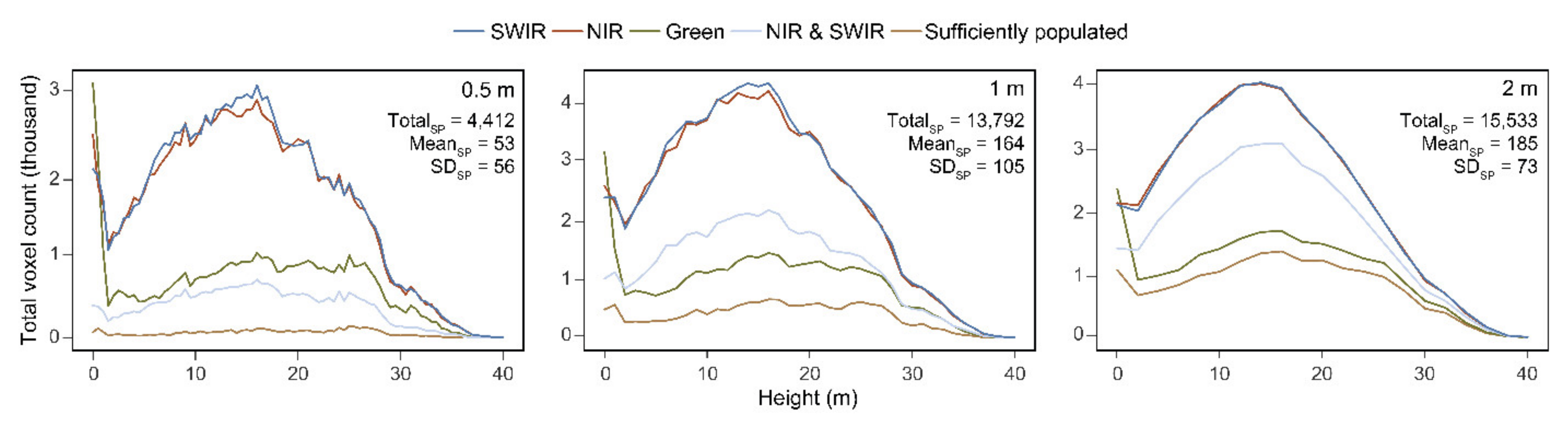
The lack of realized improvement from plot-level summaries of voxel spectral indices could be due to the observed relationship in sufficiently populated voxel counts (Figure 4). Mean counts of sufficiently populated voxels were highest for the 2 m resolution, followed by the 1 m and 0.5 m resolutions respectively (Figure 4). As resolution decreases, the total number of potentially available voxels within a plot increases; however, the chances of having a point from all three wavelengths decreases due to constriction of three-dimensional space. Unsurprisingly, the 0.5 m resolution was found to have the fewest sufficiently populated voxels, while the 2 m resolution was found to have more sufficiently populated voxels than 1 m. The difference between voxel resolution and number of sufficiently populated voxels is interesting when compared with the importance of spectral indices within diversity index models. The 1 and 2 m resolutions were found to have higher importance measures for some spectral indices, while spectral indices were not found to be important for the 0.5 m models. This indicates that voxel resolution, and the continued investigation of the potential to utilize intensity metrics from M-ALS in a three-dimensional context could improve modelling outcomes.

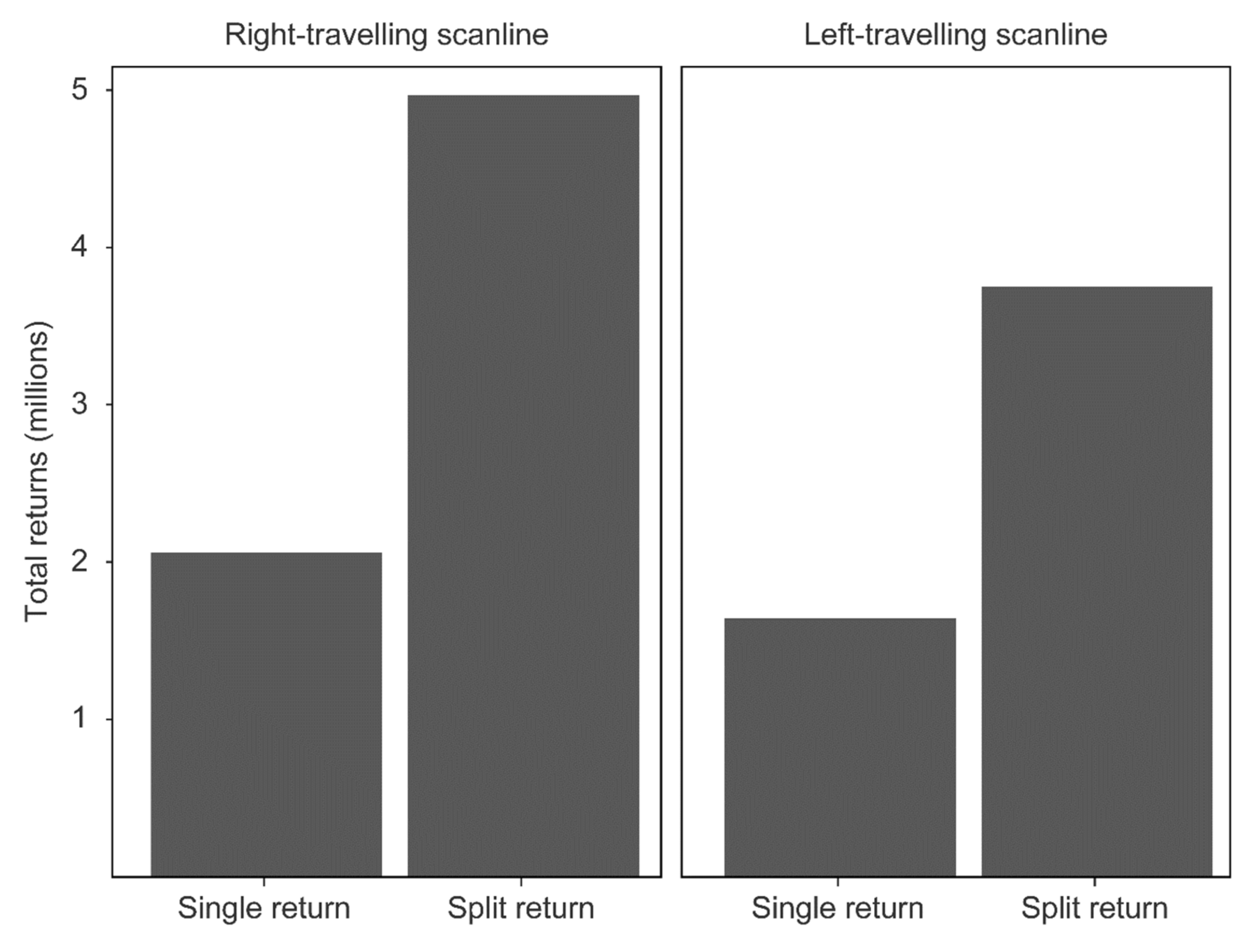
A limitation for increasing the number of sufficiently populated voxels relates to the point density of each M-ALS point cloud, the divergence of each M-ALS laser, and utilizing Optech Titan data without scanline banding effects (Table 2). The reduction in point cloud density (Table 2) following the removal of inward scanlines resulted in substantial losses to point density for each M-ALS channel. The green point cloud had much fewer points than the NIR and SWIR point clouds, which was found to be the largest limiting factor for sufficiently populated voxel counts. This is especially evident in the 2 m resolution distributions in Figure 4, where sufficiently populated voxel and green band voxel counts mimic a similar trend. Hopkinson et al. [3] noted that leaf absorption is a likely cause of reduction in the penetration of points from the green wavelength, potentially leading to the reduced number of points found in our results. Flying lower could improve the intensity based predictive results, as this would diminish the influence of attenuation on the green channel and thus normalize the return sampling densities across the three channels. Similar point densities and counts within voxels for SWIR and NIR wavelengths are likely related to their higher energy pulses.

Given that few ABA studies exist where M-ALS structure and intensity metrics are utilized, a thorough comparison to results found using individual-tree detection (ITD) approaches is not yet possible. Preliminary comparisons do, however, indicate that M-ALS intensity metrics may be better served for tree-level classification and attribute prediction applications. High modelling accuracies for species delineation in a variety of forest settings have indicated that both structure and intensity metrics improve model performance [11,26,30]. The ability for these metrics to differentiate between forest attributes and types could, therefore, be scale dependent. ABA, where metrics are summarized at the plot level, could lead to a reduced signal to those found in individually delineated tree crowns, reducing their effectiveness. Further comparisons between ABA and ITD results are needed to confirm these assumptions and to better understand the role that these M-ALS data have in forest inventory practices.

5. Conclusions

Model comparisons indicated that structural metrics from M-ALS channels were found to be most important for most forest attribute and diversity index models. Spectral metrics from M-ALS channels were found to be important for some models, particularly diversity indices, indicating potential for future the plot level studies. Voxel-based models were found to have the lowest accuracies and the inclusion of NIR_struc metrics improved forest inventory and diversity attribute estimates. The ability for M-ALS metrics to be used to differentiate between forest attributes and types is likely scale-dependent.

References

1. White, J.C.; Wulder, M.A.; Varhola, A.; Vastaranta, M.; Coops, N.C.; Cook, B.D.; Pitt, D.; Woods, M. A best practices guide for generating forest inventory attributes from airborne laser scanning data using an area-based approach. For. Chron. 2013, 89, 722–723. [Google Scholar] [CrossRef] [Green Version]
2. White, J.C.; Coops, N.C.; Wulder, M.A.; Vastaranta, M.; Hilker, T.; Tompalski, P. Remote sensing technologies for enhancing forest inventories: A review. Can. J. Remote Sens. 2016, 42, 619–641. [Google Scholar] [CrossRef] [Green Version]
3. Hopkinson, C.; Chasmer, L.; Gynan, C.; Mahoney, C.; Christopher, F.; Chasmer, L.; Gynan, C.; Mahoney, C.; Sitar, M.; Hopkinson, C.; et al. Multisensor and multispectral LiDAR characterization and classification of a forest environment multisensor and multispectral LiDAR characterization and classification of a forest environment. Can. J. Remote Sens. 2016, 45, 501–520. [Google Scholar] [CrossRef]
4. Wang, C.; Tseng, Y.; Chu, H. Airborne dual-wavelength LiDAR data for classifying land cover. Remote Sens. 2014, 6, 700–715. [Google Scholar] [CrossRef] [Green Version]
5. Kashani, A.G.; Olsen, M.J.; Parrish, C.E.; Wilson, N. A review of LIDAR radiometric processing: From ad hoc intensity correction to rigorous radiometric calibration. Sensors 2015, 15, 28099–28128. [Google Scholar] [CrossRef] [Green Version]
6. Morsy, S.; Shaker, A.; El-rabbany, A. Multispectral LiDAR data for land cover classification of urban areas. Sensors 2017, 17, 958. [Google Scholar] [CrossRef] [Green Version]
7. Charaniya, A.P.; Manduchi, R.; Lodha, S.K. Supervised parametric classification of aerial LiDAR data. In Proceedings of the IEEE Computer Society Conference on Computer Vision and Pattern Recognition Workshops, Washington, DC, USA, 27 June–2 July 2004. [Google Scholar]
8. Korpela, I.; Ole, H.; Hyyppä, J.; Heikkinen, V.; Tokola, T. Range and AGC normalization in airborne discrete-return LiDAR intensity data for forest canopies. ISPRS J. Photogramm. Remote Sens. 2010, 65, 369–379. [Google Scholar] [CrossRef]
9. Okhrimenko, M.; Coburn, C.; Hopkinson, C. Multi-spectral lidar: Radiometric calibration, canopy spectral reflectance, and vegetation vertical SVI profiles. Remote Sens. 2019, 11, 1556. [Google Scholar] [CrossRef] [Green Version]
10. Dalponte, M.; Ene, L.T.; Gobakken, T.; Næsset, E.; Gianelle, D. Predicting selected forest stand characteristics with multispectral ALS data. Remote Sens. 2018, 10, 586. [Google Scholar] [CrossRef] [Green Version]
11. Axelsson, A.; Lindberg, E.; Olsson, H. Exploring multispectral ALS data for tree species classification. Remote Sens. 2018, 10, 183. [Google Scholar] [CrossRef] [Green Version]
12. Kukkonen, M.; Maltamo, M.; Korhonen, L.; Packalen, P. Comparison of multispectral airborne laser scanning and stereo matching of aerial images as a single sensor solution to forest inventories by tree species. Remote Sens. Environ. 2019, 231, 111208. [Google Scholar] [CrossRef]
13. Jiang, C.; Chen, Y.; Wu, H.; Li, W.; Zhou, H.; Bo, Y.; Shao, H.; Song, S.; Puttonen, E.; Hyyppä, J. Study of a high spectral resolution hyperspectral LiDAR in vegetation red edge parameters extraction. Remote Sens. 2019, 11, 2007. [Google Scholar] [CrossRef] [Green Version]
14. Zhang, C.; Gao, S.; Niu, Z.; Pei, J.; Bi, K.; Sun, G. Calibration of the pulse signal decay effect of full-waveform hyperspectral LiDAR. Sensors 2019, 19, 5263. [Google Scholar] [CrossRef] [PubMed] [Green Version]
15. Vauhkonen, J.; Hakala, T.; Suomalainen, J.; Kaasalainen, S.; Nevalainen, O. Classification of spruce and pine trees using active hyperspectral LiDAR. IEEE Geosci. Remote Sens. Lett. 2013, 10, 1138–1141. [Google Scholar] [CrossRef]
16. Nevalainen, O.; Hakala, T.; Suomalainen, J.; Mäkipää, R. Agricultural and forest meteorology fast and nondestructive method for leaf level chlorophyll estimation using hyperspectral LiDAR. Agric. For. Meteorol. 2014, 198–199, 250–258. [Google Scholar] [CrossRef]
17. Hakala, T.; Suomalainen, J.; Kaasalainen, S.; Chen, Y. Full waveform hyperspectral LiDAR for terrestrial laser scanning. Opt. Express 2012, 20, 422–430. [Google Scholar] [CrossRef]
18. Stone, C.; Mohammed, C. Application of remote sensing technologies for assessing planted forests damaged by insect pests and fungal pathogens: A review. Curr. For. Rep. 2017, 3, 75–92. [Google Scholar] [CrossRef]
19. Dash, J.; Pearse, G.; Watt, M. UAV multispectral imagery can complement satellite data for monitoring forest health. Remote Sens. 2018, 10, 1216. [Google Scholar] [CrossRef] [Green Version]
20. Hilker, T.; Wulder, M.A.; Coops, N.C. Update of forest inventory data with lidar and high spatial resolution satellite imagery. Can. J. Remote Sens. 2008, 34, 5–12. [Google Scholar] [CrossRef]
21. Matasci, G.; Hermosilla, T.; Wulder, M.A.; White, J.C.; Coops, N.C.; Hobart, G.W.; Bolton, D.K.; Tompalski, P.; Bater, C.W. Three decades of forest structural dynamics over Canada’s forested ecosystems using Landsat time-series and lidar plots. Remote Sens. Environ. 2018, 216, 697–714. [Google Scholar] [CrossRef]
22. Hermosilla, T.; Wulder, M.A.; White, J.C.; Coops, N.C.; Hobart, G.W. Disturbance-informed annual land cover classification maps of Canada’s forested ecosystems for a 29-year landsat time series. Can. J. Remote Sens. 2018, 44, 67–87. [Google Scholar] [CrossRef]
23. Goodbody, T.R.H.; Coops, N.C.; White, J.C. Digital aerial photogrammetry for updating area-based forest inventories: A review of opportunities, challenges, and future directions. Curr. For. Rep. 2019, 5, 55–75. [Google Scholar] [CrossRef] [Green Version]
24. Tompalski, P.; White, J.C.; Coops, N.C.; Wulder, M.A. Quantifying the contribution of spectral metrics derived from digital aerial photogrammetry to area-based models of forest inventory attributes. Remote Sens. Environ. 2019, 234, 111434. [Google Scholar] [CrossRef]
25. Rahlf, J.; Breidenbach, J.; Solberg, S.; Næsset, E.; Astrup, R. Remote sensing of environment comparison of four types of 3D data for timber volume estimation. Remote Sens. Environ. 2014, 155, 325–333. [Google Scholar] [CrossRef]
26. Budei, B.C.; St-Onge, B.; Hopkinson, C.; Audet, F. Remote sensing of environment identifying the genus or species of individual trees using a three-wavelength airborne lidar system. Remote Sens. Environ. 2018, 204, 632–647. [Google Scholar] [CrossRef]
27. Chen, X.; Ye, C.; Li, J.; Member, S.; Chapman, M.A. Quantifying the carbon storage in urban trees using multispectral ALS data. IEEE J. Sel. Top. Appl. Earth Obs. Remote Sens. 2018, 11, 3358–3365. [Google Scholar] [CrossRef]
28. Kukkonen, M.; Maltamo, M.; Korhonen, L.; Packalen, P. Multispectral airborne LiDAR data in the prediction of boreal tree species composition. IEEE Trans. Geosci. Remote Sens. 2019, 57, 3462–3471. [Google Scholar] [CrossRef]
29. Okhrimenko, M.; Hopkinson, C. Investigating the consistency of uncalibrated multispectral lidar vegetation indices at different altitudes. Remote Sens. 2019, 11, 1531. [Google Scholar] [CrossRef] [Green Version]
30. Yu, X.; Hyyppä, J.; Litkey, P.; Kaartinen, H.; Vastaranta, M. Single-sensor solution to tree species classification using multispectral airborne laser scanning. Remote Sens. 2017, 9, 108. [Google Scholar] [CrossRef] [Green Version]
31. Næsset, E. Predicting forest stand characteristics with airborne scanning laser using a practical two-stage procedure and field data. Remote Sens. Environ. 2002, 80, 88–99. [Google Scholar] [CrossRef]
32. White, J.C.; Chen, H.; Woods, M.E.; Low, B.; Nasonova, S. The petawawa research forest: Establishment of a remote sensing supersite. For. Chron. 2019, 95, 149–156. [Google Scholar] [CrossRef] [Green Version]
33. Penner, M.; Woods, M. LiDAR Stand-Level Predictions for the PRF; Ontario Ministry of Natural Resources and Forestry: Peterborough, ON, Canada, 2015; Unpublished work. [Google Scholar]
34. Van Ewijk, K.; Treitz, P.; Woods, M.; Jones, T.; Caspersen, J. Forest site and type variability in ALS-based forest resource inventory attribute predictions over three Ontario forest sites. Forests 2019, 10, 226. [Google Scholar] [CrossRef] [Green Version]
35. Goodbody, T.R.H.; Coops, N.C.; Hermosilla, T.; Tompalski, P.; McCartney, G.; MacLean, D.A. Digital aerial photogrammetry for assessing cumulative spruce budworm defoliation and enhancing forest inventories at a landscape-level. ISPRS J. Photogramm. Remote Sens. 2018, 142, 1–11. [Google Scholar] [CrossRef]
36. Yan, W.Y.; Shaker, A. Airborne LiDAR intensity banding: Cause and solution. ISPRS J. Photogramm. Remote Sens. 2018, 142, 301–310. [Google Scholar] [CrossRef]
37. Roussel, J.-R.; Auty, D. LidR: Airborne LiDAR Data Manipulation and Visualization for Forestry Applications. R package version 2.2.4. 2018. Available online: https://CRAN.R-project.org/package=lidR (accessed on 30 June 2020).
38. Hunt, E.; Doraiswamy, P.; McMurtrey, J.E.; Daughtry, C.S.; Perry, E.; Akhmedov, B. A visible band index for remote sensing leaf chlorophyll content at the Canopy scale. Int. J. Appl. Earth Obs. Geoinf. 2012, 21, 103–112. [Google Scholar] [CrossRef] [Green Version]
39. Bush, B.L.; Nachbar, R.B. Sample-distance partial least squares: PLS optimized for many variables, with application to CoMFA. J. Comput. Aided Mol. Des. 1993, 7, 587–619. [Google Scholar] [CrossRef] [PubMed]
40. Van den Berg, R.A.; Hoefsloot, H.C.J.; Westerhuis, J.A.; Smilde, A.K.; van der Werf, M.J. Centering, scaling, and transformations: Improving the biological information content of metabolomics data. BMC Genom. 2006, 7, 142. [Google Scholar] [CrossRef] [Green Version]
41. Kuhn, M.; Wing, J.; Weston, S.; Williams, A.; Keefer, C.; Engelhardt, A.; Cooper, T.; Mayer, Z.; Kenkel, B.; Team, R.C.; et al. Caret: Classification and Regression Training. 2019. Available online: https://CRAN.R-project.org/package=caret (accessed on 30 June 2020).
42. Strobl, C.; Boulesteix, A.-L.; Kneib, T.; Augustin, T.; Zeileis, A. Conditional variable importance for random forests. BMC Bioinform. 2008, 9, 307. [Google Scholar] [CrossRef] [Green Version]
43. Strobl, C.; Boulesteix, A.L.; Zeileis, A.; Hothorn, T. Bias in random forest variable importance measures: Illustrations, sources and a solution. BMC Bioinform. 2007, 8, 25. [Google Scholar] [CrossRef] [Green Version]
44. Robinson, A.P.; Duursma, R.A.; Marshall, J.D. A regression-based equivalence test for model validation: Shifting the burden of proof. Tree Physiol. 2005, 25, 903–913. [Google Scholar] [CrossRef]
45. Robinson, A.P.; Froese, R.E. Model validation using equivalence tests. Ecol. Model. 2004, 176, 349–358. [Google Scholar] [CrossRef]
46. Robinson, A. Equivalence: Provides Tests and Graphics for Assessing Tests of Equivalence. 2016. Available online: https://CRAN.R-project.org/package=equivalence (accessed on 30 June 2020).
47. Penner, M.; Pitt, D.G.; Woods, M.E. Parametric vs. nonparametric LiDAR models for operational forest inventory in boreal Ontario. Can. J. Remote Sens. 2013, 39, 426–443. [Google Scholar] [CrossRef]
48. Fekety, P.A.; Falkowski, M.J.; Hudak, A.T.; Jain, T.B.; Evans, J.S. Transferability of lidar-derived basal area and stem density models within a northern Idaho ecoregion. Can. J. Remote Sens. 2018, 44, 131–143. [Google Scholar] [CrossRef]
49. Gallus, L.; Hill, A.; Waser, L.T.; Bürgi, A.; Ginzler, C.; Blattert, C. Forest ecology and management airborne-laser-scanning-derived auxiliary information discriminating between broadleaf and conifer trees improves the accuracy of models for predicting timber volume in mixed and heterogeneously structured forests. For. Ecol. Manag. 2020, 459, 117856. [Google Scholar] [CrossRef]
Figure 1. Relief map of the Petawawa Research Forest. Black markers indicate field plot locations.
Remotesensing 12 02109 g001
Figure 2. Comparison of return frequency between right-traveling (relative to flight path) and left-traveling scanline directions.
Remotesensing 12 02109 g002
Figure 3. Graphical description of methods.
Remotesensing 12 02109 g003
Figure 4. Total count of voxels for all plots containing at least one point for each M-ALS wavelength individually, where NIR and SWIR were both contained within a voxel, and sufficiently populated (SP) voxels with points from all bands. Descriptive statistics indicate the total number of SP voxels, as well as the mean and standard deviation (SD) of SP voxels per plot.
Remotesensing 12 02109 g004