Leaf Area Index Estimation Algorithm for GF-5 Hyperspectral Data Based on Different Feature Selection and Machine Learning Methods

Abstract

Leaf area index (LAI) is an essential vegetation parameter that represents the light energy utilization and vegetation canopy structure. As the only in-operation hyperspectral satellite launched by China, GF-5 is potentially useful for accurate LAI estimation. However, there is no research focus on evaluating GF-5 data for LAI estimation. Hyperspectral remote sensing data contains abundant information about the reflective characteristics of vegetation canopies, but these abound data also easily result in a dimensionality curse. Therefore, feature selection (FS) is necessary to reduce data redundancy to achieve more reliable estimations. Currently, machine learning (ML) algorithms have been widely used for FS. Moreover, the same ML algorithm is usually conducted for both FS and regression in LAI estimation. However, no evidence suggests that this is the optimal solution. Therefore, this study focuses on evaluating the capacity of GF-5 spectral reflectance for estimating LAI and the performances of different combination of FS and ML algorithms. Firstly, the PROSAIL model, which coupled leaf optical properties model PROSPECT and the scattering by arbitrarily inclined leaves (SAIL) model, was used to generate simulated GF-5 reflectance data under different vegetation and soil conditions, and then three FS methods, including random forest (RF), K-means clustering (K-means) and mean impact value (MIV), and three ML algorithms, including random forest regression (RFR), back propagation neural network (BPNN) and K-nearest neighbor (KNN) were used to develop nine LAI estimation models. The FS process was conducted twice using different strategies: Firstly, three FS methods were conducted to search the lowest dimension number, which maintained the estimation accuracy of all bands. Then, the sequential backward selection (SBS) method was used to eliminate the bands having minimal impact on LAI estimation accuracy. Finally, three best estimation models were selected and evaluated using reference LAI. The results showed that although the RF_RFR model (RF used for feature selection and RFR used for regression) achieved reliable LAI estimates (coefficient of determination (R²) = 0.828, root mean square error (RMSE) = 0.839), the poor performance (R² = 0.763, RMSE = 0.987) of the MIV_BPNN model (MIV used for feature selection and BPNN used for regression) suggested using feature selection and regression conducted by the same ML algorithm could not always ensure an optimal estimation. Moreover, RF selection preserved the most informative bands for LAI estimation so that each ML regression method could achieve satisfactory estimation results. Finally, the results indicated that the RF_KNN model (RF used as feature selection and KNN used for regression) with seven GF-5 spectral band reflectance achieved the better estimation results than others when validated by simulated data (R² = 0.834, RMSE = 0.824) and actual reference LAI (R² = 0.659, RMSE = 0.697).

1. Introduction

Leaf area index (LAI), which is defined as the ratio of total leaf area per unit of horizontal ground surface area, is one of the key input parameters of numerous ecosystem models [1,2,3]. Since it can characterize the substance and energy exchange in vegetation canopy, LAI is also regarded as an essential indicator of vegetation condition, productivity and photosynthetic capacity [4]. Therefore, accurate LAI estimation at different scales (regional and global) is crucial for many applications, such as climate change, crop yield modeling, and ecological monitoring [5,6,7].

Remote sensing data with superiority in extensive coverage and nondestructive estimation provide effective information for LAI estimation at the regional scale [8]. Therefore, accurate LAI estimation becomes an essential issue in the field of quantitative remote sensing [9,10]. Recently, many global and regional LAI estimation algorithms have been proposed using different multispectral satellite data such as moderate resolution imaging spectroradiometer (MODIS), Satellite Pour l’ Observation de la Terre (SPOT) VEGETATION, Landsat, Sentinel and GF-1 [11,12,13,14,15,16,17]. However, some studies show that the saturation phenomenon occurred in LAI estimation when using multispectral band reflectance or vegetation indices (VIs) [18,19,20]. In contrast, hyperspectral sensors acquire remote sensing data with hundreds of consecutive narrow bands that have the capacity of detecting small changes in light absorption and reflection [21,22]. Previous studies have shown that hyperspectral reflectance or VIs can estimate forest aboveground biomass [23], LAI [24,25], fractional vegetation cover (FVC) [26] and leaf chlorophyll content (LCC) accurately [27]. Some of them even indicated that it could resolve the underestimation problem in LAI estimation [28,29]. However, since just a few hyperspectral satellite data are available, most studies are conducted by airborne hyperspectral equipment or ground-based spectral devices. However, those devices are limited to the spatial coverage. Therefore, as the only in-operation hyperspectral satellite launched by China, GF-5 has a great potential for LAI estimation in a large area. Unfortunately, there is scarcely any study for LAI estimation using GF-5 data.

Although GF-5 hyperspectral data describe more details about absorption features of canopy or leaves than multispectral data, the contiguous bands also easily result in spectral autocorrelation, which is also known as “high dimensional disaster” or “Hughes” [30,31]. Therefore, dimensionality reduction methods are usually applied to overcome data redundancy, improve computational efficiency and reduce the risk of overfitting [32,33,34,35]. There are two different ways of dimensionality reduction: one is called feature extraction (FE), which is conducted to transform the original data into other feature spaces that allow the generated low-dimensional data contain the vast majority of information [36,37,38], such as principal component analysis (PCA). However, despite the principal components (PCs) obtained by those methods are independent with each other, the meaning of each PC is not as clear as the original data. Moreover, the PCs with small variance may contain important information on sample differences, thus, discarding that information may have an impact on final LAI estimation accuracy. The other dimensionality reduction approach is known as feature selection (FS), which is conducted to select a group of features that contains the most important and useful information of the original data set [39]. For instance, methods like simulated annealing (SA) [40], genetic algorithms (GA) [41] and correlation-based feature selection (CFS) [42] belong to this category. Compared with FE, FS methods not only can avoid the curse of dimensionality but also maintain the original data characteristics, which makes the results more interpretable. The purpose of dimensionality reduction is to eliminate the negative impact of redundant features and improve model performance. However, other than dimensionality reduction methods, the regression algorithm is another crucial aspect that also has a great influence on LAI estimation accuracy. Some machine learning (ML) algorithms possess the ability in both feature selection and regression. For instance, random forest (RF) [43] has its own built-in feature selection method that can derive the importance of each variable on the tree decision. Thus, the contribution of each variable to the estimation can be easily understood. RankSVM and kernel RankSVM [44,45], which are extended from the basic support vector machine (SVM) [46], ranking the features according to the performance of evaluation criterion such as root mean square error (RMSE). However, although those ML algorithms can be used in feature selection and regression, there is no evidence shows that using the same algorithm for feature selection and regression would achieve more accurate estimations. Therefore, the LAI estimation performance of different FS and ML regression combinations is still worth discussing.

In this study, three different FS methods with different searching standard, including K-means, RF and mean impact value (MIV), and three ML regression algorithms, including RF regression (RFR), back propagation neural network (BPNN) and K-nearest neighbor (KNN), were combined and compared to develop the LAI estimation algorithm for GF-5 hyperspectral data. For this purpose, the radiative transfer model PROSAIL [47], which coupled leaf optical properties model PROSPECT and the scattering by arbitrarily inclined leaves (SAIL), was used to generate a simulated data set of GF-5 band reflectance and corresponding LAI values under different conditions. Then, FS process was conducted to find the best input variables for LAI estimation. Finally, three best LAI estimation models for GF-5 hyperspectral data were selected and evaluated using reference LAI.

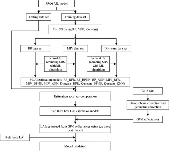
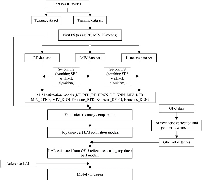
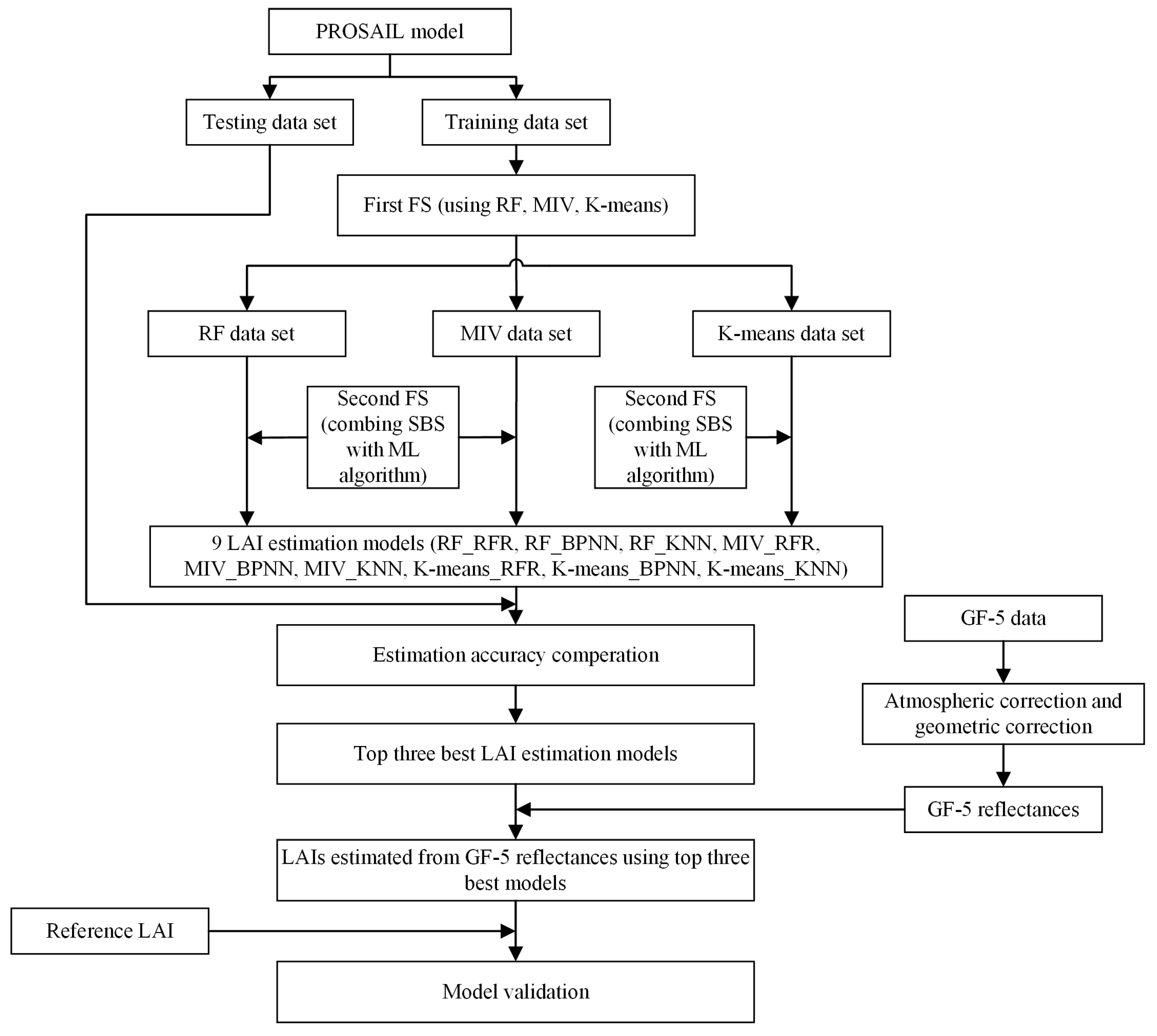
2. Materials and Methods

Figure 1 shows the experiment workflow of this study. Firstly, the PROSAIL model was used to generate a number of simulated data that consist of the training and testing data sets. Then, the first FS process was used to select three different subsets (RF data set, MIV data set and K-means data set), and the second FS process, which combines the sequential backward selection (SBS) process with ML regression, was conducted to select the final variables for LAI estimation. Next, the testing data set was applied to select the top three best LAI estimation models. Finally, LAI was estimated using GF-5 reflectance by the three models and evaluated using the reference LAI data.

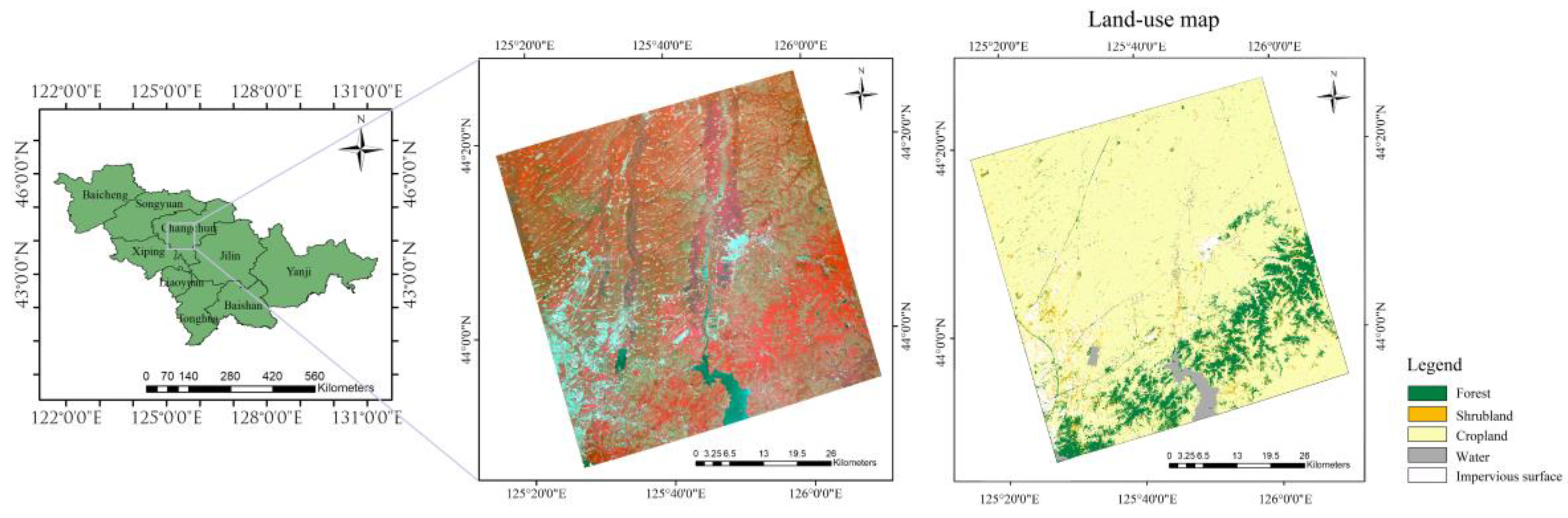
2.1. Study Area and Field Survey

The study area that covers approximately 3760 km² is located in Changchun (43°05′N–45°15′N; 124°18′E–127°05′E), Jilin province of China (Figure 2). It has a flat terrain with an altitude varying from 137 to 160 m. The temperate continental humid climate type with annual precipitation range from 600 to 700 mm in this region is very suitable for crop growth. Field maize LAI measurements were collected from 16 to 21 July, 2019. There are 26 sample plots with size of 20 m × 20 m and seven LAI values were measured using a LAI-2200C plant canopy analyzer (LI-COR Inc., Lincoln, Nebraska) in each plot. However, not all of the measured LAI values could be used in this study because of the availability of GF-5 hyperspectral data. Therefore, Sentinel-2 data were firstly used to estimate LAI, and then both the Sentinel-2 LAI estimates and measured LAI values were regarded as a reference LAI to evaluate the estimation accuracy of each GF-5 model.

2.2. Data Pre-Processing

2.2.1. Sentinel-2 Data

Sentinel-2 is a widely used satellite launched by the European Space Agency (ESA) in June 2015 [48,49]. Users can search and download Sentinel-2 data from the Copernicus Open Access Hub. The Multi Spectral Instruments (MSI) installed in this satellite provide 13 spectral bands ranged from visible (VIS) to shortwave infrared (SWIR). Sentinel-2 has three different high spatial resolutions. For example, Band 1 (coastal aerosol), Band 9 (water vapor) and Band 10 (SWIR-Cirrus) have a spatial resolution of 60 m. While four vegetation RE bands (Band 5, 6, 7 and 8a) and two SWIR bands (Band 11 and 12) have a spatial resolution of 20 m. The last four bands (Band 2, 3, 4 and 8) that have a distribution in VIS and NIR have a spatial resolution of 10 m.

In this study, the sample plots were fully covered by one Sentinel-2B MSIL2A data (tile number 51TXK). To obtain high accuracy reference LAI, bands with 10 and 20 m spatial resolution, which are proven to be very useful in LAI estimation [50,51,52], were used in this study.

2.2.2. GF-5 Hyperspectral Data

The GF-5, which was launched in May 2018 from Taiyuan Satellite Launch Centre, is the only hyperspectral satellite in the China High-resolution Earth Observation System. Compared with other GF satellites, GF-5 is also the only one that carries six different sensors for various academic and application use. Among all the sensors carried by GF-5, the visible-shortwave infrared advanced hyperspectral imager (AHSI) is the main payload, which was used to obtain 330 bands ranging from 400 to 2500 nm, with 30 m spatial resolution and 60 km swath width. There are two different spectral resolutions of those bands: 5 nm in VNIR and 10 nm in SWIR. Compared to the Hyperion Imaging Spectrometer [53,54], which is also a hyperspectral satellite sensor (with spectral resolution of 10 nm and band number of 224), GF-5 not only provides more detailed information, but also has a higher signal-to-noise ratio, which guarantees better data quality.

GF-5 hyperspectral data can be searched from the Land Observation Satellite Service website. In this study, ortho-rectification and atmospheric correction are conducted to obtain the GF-5 land surface reflectance. After removing the invalid bands, overlapped bands in the SWIR region and blue bands, which are seriously affected by atmospheric scattering, 210 bands were selected for further LAI estimation algorithm development.

2.3. Using PROSAIL Model to Generate Simulated Data

PROSAIL model [55] is widely used in biophysical parameters estimation because of its high accuracy and computing efficiency [56,57]. In the PROSAIL model, the PROSPECT model was used to simulate the reflectance and transmittance of leaves from 400 to 2500 nm. Then the spectral information of leaves is regarded as the input of the SAIL model to generate canopy reflectance [56]. Since the parameter setting will affect the calculation speed and the redundancy of outputs, reasonable ranges and fixed values were applied according to the previous studies [58,59] (

Table 1. The parameter setting of the PROSAIL model [57].

Model	Parameters	Units	Min	Max	Distribution
PROSPECT	Cab	µg/cm2	20	90	Uniform
	Cm	g/cm2	0.003	0.0011	Uniform
	Car	µg/cm2	4.4	4.4	-
	Cw	cm	0.005	0.015	Uniform
	Cbrown	-	0	2	Uniform
	Cant	µg/cm2	0	0	-
	N	-	1.2	2.2	Uniform
SAIL	LAI	-	0	7	Uniform
	ALA	°	30	70	Uniform
	SZA	°	35	35	-
	Hot	-	0.1	0.5	Uniform

In Table 1, C_ab, C_m, C_ar, C_w, C_brown, C_ant, N, LAI, ALA, SZA and Hot represent the leaf chlorophyll a + b concentration, dry matter content, carotenoid content, equivalent water thickness, brown pigment content, anthocyanin content, leaf structure parameter, leaf area index, average leaf angle inclination, solar zenith angle and hot-spot parameter, respectively.

).

As the representation of underlying surface information, soil reflectance is also a vital parameter for the PROSAIL model. In this study, 20 representative soil reflectance were generated from the International Soil Reference and Information Center (http://www/isric.org) using the method proposed by Wang et al. [57].

After simulating canopy reflectance at 400–2500 nm wavelength, resampling was conducted to obtain GF-5 band reflectance according to the center wavelength and bandwidth of the selected bands. Compared with the simulated data, canopy reflectance of plants driven by the satellite contains some noise generated by the sensors. Therefore, a Gaussian white noise of 1% was added into the simulated data [57,60]. The training set and validation set were produced separately. Considering the computational efficiency, the simulation generated 24,000 samples as a training set and 4800 samples as a validation set.

2.4. Feature Selection Methods

Feature selection is one of the core concepts in machine learning, which highly influences the model performance. In this study, three FS methods with different criteria (RF, MIV and K-means) were applied to the original data set to determine the appropriate dimension number, which still maintains satisfactory LAI estimation accuracy. Then, the SBS method was used to search for the optimal subsets for LAI estimation.

2.4.1. RF for Feature Selection

Random forest is one of the most popular and efficient algorithms for regression and classification problems. Different from other machine learning algorithms, RF combines the idea of bagger with random feature selection [61,62,63]. Based on the information of the randomly selected samples, RF can predict the category (for classification) and value (for regression) of the target by establishing multiple independent decision trees [64]. It achieves the final result and out-of-bag (OOB) error by voting for the independent results of decision trees. The OOB error not only indicates the accuracy of RF model but also can be used to evaluate the classification and estimation capacity of each variable. In the end, the RF model would output the importance score of each variable. Then users can choose the suitable variable subset according to the predefined dimension or accuracy.

2.4.2. MIV

MIV is another feature selection algorithm that belongs to the embedded category like RF. This method assesses each variable by testing their stability of estimation performance by adding noise to the original data set. The major steps are as follows [65,66]:

Step 1: Training network using BPNN algorithm, and then recording outputs as $A_i$;

Step 2: Every input variable value ($P_i$) in the original training data set was transformed by increasing and decreasing 10% to form new training data sets.

$$P_{i1}=1.1\times P_i,P_{i2}=0.9\times P_i$$

(1)

Step 3: Taking $P_{i1}$ and $P_{i2}$ as input data, then training those data using network obtained in step 1. The output is recorded as $A_{i1}$ and $A_{i2}$. Calculating the difference value between $A_{ij}$ and $P_{ij}$, and recording as impact value (IV):

$$I{V}_{i1}=A_{i1}-A_i,I{V}_{i2}=A_{i2}-A_i$$

(2)

Step 4: Calculating the mean value of IV (MIV) according to the number of samples, and then outputting the MIV for each variable. Finally, the variables are ranked according to the magnitude of the absolute value of MIV.

2.4.3. K-means

K-means is a simply and efficient iterative clustering algorithm that can be used as the dimensional reduction algorithm without label information [67,68]. Unlike RF and MIV, K-means need to combine with alternative criteria such as the feature correlation index, mutual information [69] to achieve the final results. In this study, the Pearson correlation coefficient (PCC) between the input variable and LAI was used as criteria for K-means feature selection. The main steps are as follows:

Step 1: Selecting k initial clustering centers randomly in feature space;

Step 2: Calculating the distance between each feature and cluster center, then classifying them into the closest category;

Step 3: Calculating the average value of all data in each category, then using this value to determine the new center of each category;

Step 4: Evaluating the astringency of the clustering function based on the category center. Final clustering result will be obtained when the function is convergent;

Step 5: Calculating the PCC between each variable and LAI, and then selecting the variable with the highest PCC value in each category as the FS result.

2.5. Machine Learning Algorithm

2.5.1. RFR

Random forest regression is an ensemble learning technique developed by Breiman [70]. This algorithm achieves more accurate and stable results by combining the individual results of a large number of decision trees [71]. RFR uses a bootstrap resampling method to extract a number of sample sets (k) from the original data set, and then takes each set as a training sample to generate a single decision tree. Every node variable at each split of decision tree is the best one chosen from the input variables (m). The final estimation result is determined by the average value of each prediction result of decision trees [72]. The number of sample sets (k) and the number of input variables (m) need to be set by users in the RFR model. After several tests, those two parameters were set to 1/3 and 500, respectively.

2.5.2. BPNN

The back propagation neural network [73] is one of the effective and widely used neural networks for vegetation parameter estimation [74,75,76,77,78]. The construction of this network is mainly achieved by training the weights with a non-linear differentiable function. The basic concept of BPNN is to adjust the network parameters by calculating the error between outputs and the expected values to improve accuracy. This study adopted the three-layer network with a single hidden layer. Each layer is connected by different functions. In this BPNN model, “tansig” is selected as the activation function to construct a nonlinear mapping between the input layer and hidden layer, “pureline” is selected as the transfer function to build a linear mapping between the hidden layer and output layer, and “trainlm” is selected as the training function.

The number of nodes (n) in the hidden layer is an important factor affecting fitting accuracy. In this study, the number of nodes in the input layer (n_i) was equal to the dimension of the subset that was selected by FS methods, and the output had one node (n₀), which corresponded to the LAI values. The number of nodes in the hidden layer can be determined using Equation (5). Since a in Equation (5) ranged from 1 to 10, the number of nodes in the hidden layer needs to be determined by evaluating every possible value, and 15 was determined as the optimal value of n.

$$n=\sqrt{n_i+n_0}+a$$

(3)

2.5.3. KNN

KNN is one of the simple ML methods that determine the sample characteristic by considering the performance of its nearest neighbors [79]. It is not only suitable for classification, but also for quantitative estimation of vegetation parameters [80]. Since KNN does not depend on specific function distribution, it is suitable for feature fusion and missing value estimation of multi-mode remote sensing. The attribute values of the estimation pixels are obtained by weighting k pixels that are nearest to them. The formula is as follows:

$$V_p={\displaystyle \sum _{i=1}^k{W}_{p,pi}{V}_{pi}},1\le i\le k$$

(4)

where V_p and V_pi represent the attribute value of estimation pixel p and k pixels named pi; W_p,pi represents the weight between p and pi. In this study, W_p,pi is defined by Euclidean distance.

In general, KNN estimates the value of the validation samples by taking average of some training data. Therefore, the estimation accuracy of KNN model depends on the parameter k, which represents the size of the training data near to the validation sample [81]. In this study, 10-fold cross-validation was introduced to find optimal k in which the search range was set to 2–20.

In this study, three feature selection methods and three machine learning algorithms generate nine LAI estimation models, and their abbreviations and descriptions are shown in

Table 2. The abbreviations and descriptions of nine LAI estimation models.

Model	Description
RF_RFR	Using the random forest algorithm as feature selection and regression methods.
RF_BPNN	Using the random forest algorithm and back propagation neural network algorithm as feature selection method and regression method, respectively.
RF_KNN	Using the random forest algorithm and K-nearest neighbor algorithm as the feature selection method and regression method, respectively.
MIV_RFR	Using the mean impact value algorithm and random forest regression algorithm as the feature selection method and regression method, respectively.
MIV_BPNN	Using the mean impact value algorithm and back propagation neural network algorithm as the feature selection method and regression method, respectively.
MIV_KNN	Using the mean impact value algorithm and K-nearest neighbor algorithm as the feature selection method and regression method, respectively.
K-menas_RFR	Using the K-means algorithm and random forest regression algorithm as the feature selection method and regression method, respectively.
K-means_BPNN	Using the K-means algorithm and back propagation neural network algorithm as the feature selection method and regression method, respectively.
K-means_KNN	Using the K-means algorithm and K-nearest neighbor algorithm as the feature selection method and regression method, respectively.

.

2.6. LAI Estimation Accuracy Evaluation

In this study, model validation consisted of two different parts. Firstly, the validation set that contained 4800 simulated samples was used to access the performance of different FS and ML combinations for LAI estimation. Secondly, the reference LAI contained field LAI measurements and Sentinel-2 data derived LAI values were used for LAI estimation accuracy assessment of actual GF-5 hyperspectral data. The reference LAI values from Sentinel-2 were also obtained by PROSAIL and machine learning algorithms. Firstly, PROSAIL model was used to generate simulated data including Sentinel-2 reflectance and corresponding LAI. Then, nine spectral band reflectance (Band 2 to Band 8a, Band 11 and Band 12) and five vegetation indices (

Table 3. Vegetation indexes of Sentinel-2.

Vegetation Index	Abbreviation	Formula
Normalized Difference Vegetation Index	NDVI	(Band8 − Band4)/(Band8 + Band4)
Normalized Difference Red Edge Index 1	NDRE1	(Band8 − Band5)/(Band8 + Band5)
Normalized Difference Red Edge Index 2	NDRE2	(Band8 − Band6)/(Band8 + Band6)
Normalized Difference Red Edge Index 3	NDRE3	(Band8 − Band7)/(Band8 + Band7)
Normalized Difference Red Edge Index 4	NDRE4	(Band8 − Band8a)/(Band8 + Band8a)

) were selected as input variables. To prevent the ML regression method used in the Sentinel-2 LAI estimation model from affecting the validation of GF-5 LAI estimation, RFR, BPNN and KNN were all used to estimate LAI from Sentinel-2 data and the average values of the three models were determined as the reference LAI (Figure 3). The reference LAI achieved satisfactory estimation accuracy with R² of 0.506 and RMSE of 0.679. Therefore, the Sentinel-2 derived LAI could be used as a reference to access the accuracy of LAI estimation models using GF-5 data.

The coefficient of determination (R²) and root mean square error (RMSE) were used to verify the LAI estimation accuracy of each model. The computing formulas are as follows:

$$R^2=1\frac{{\displaystyle \sum _{i=1}^n{(y_i-y_i^{\prime })}^2}}{{\displaystyle \sum _{i=1}^n{(y_i-\overline{y})}^2}}$$

(5)

$$RMSE={[\frac{1}{n}{\displaystyle \sum _{i=1}^n{(y_i-y_i^{\prime })}^2}]}^{1/2}$$

(6)

where $y_i$, $y_i^{\prime }$ $\overline{y}$ and $n$ represent the reference LAI value, estimated LAI value, average of the reference LAI value and the number of samples.

3. Results

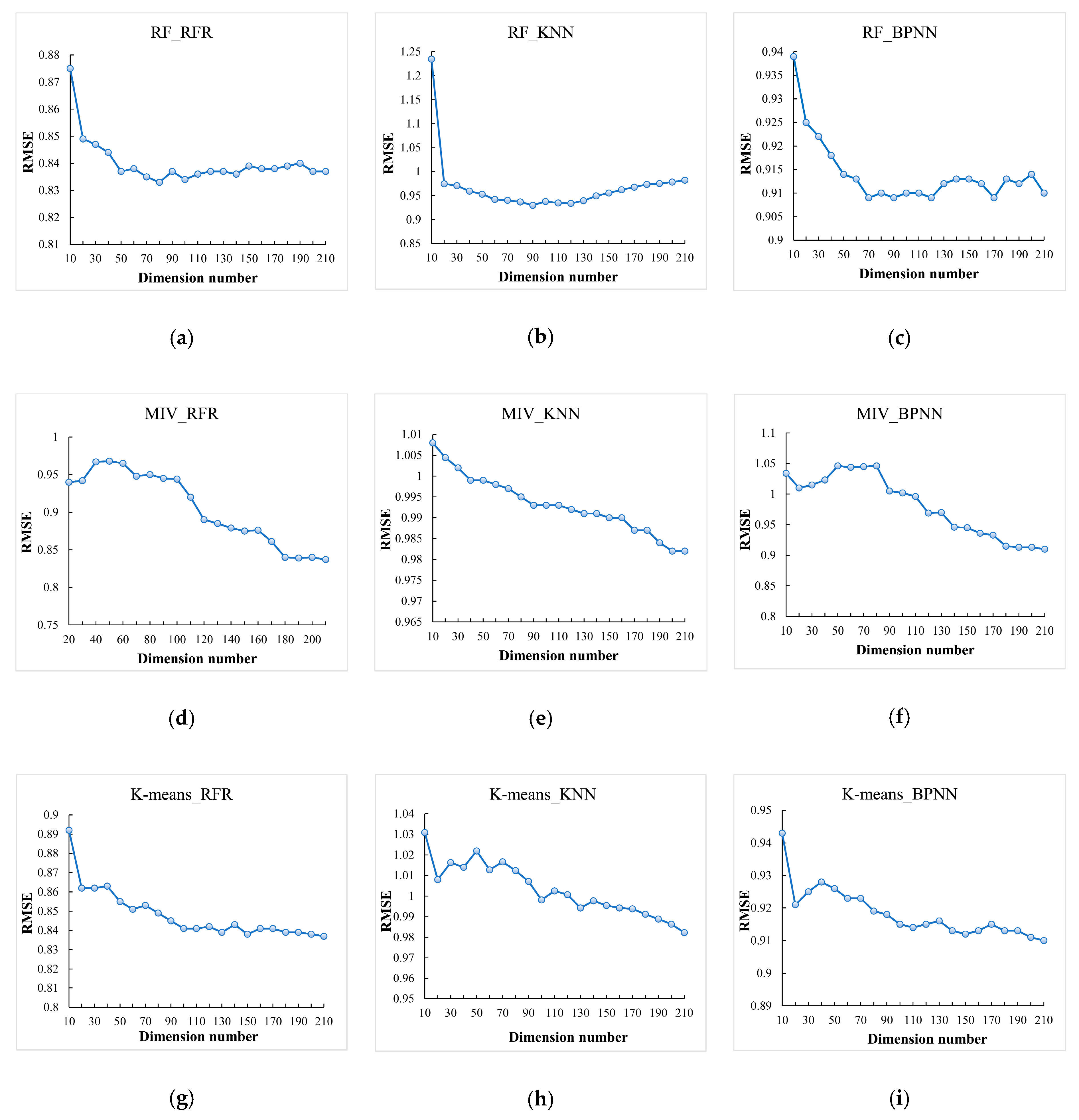
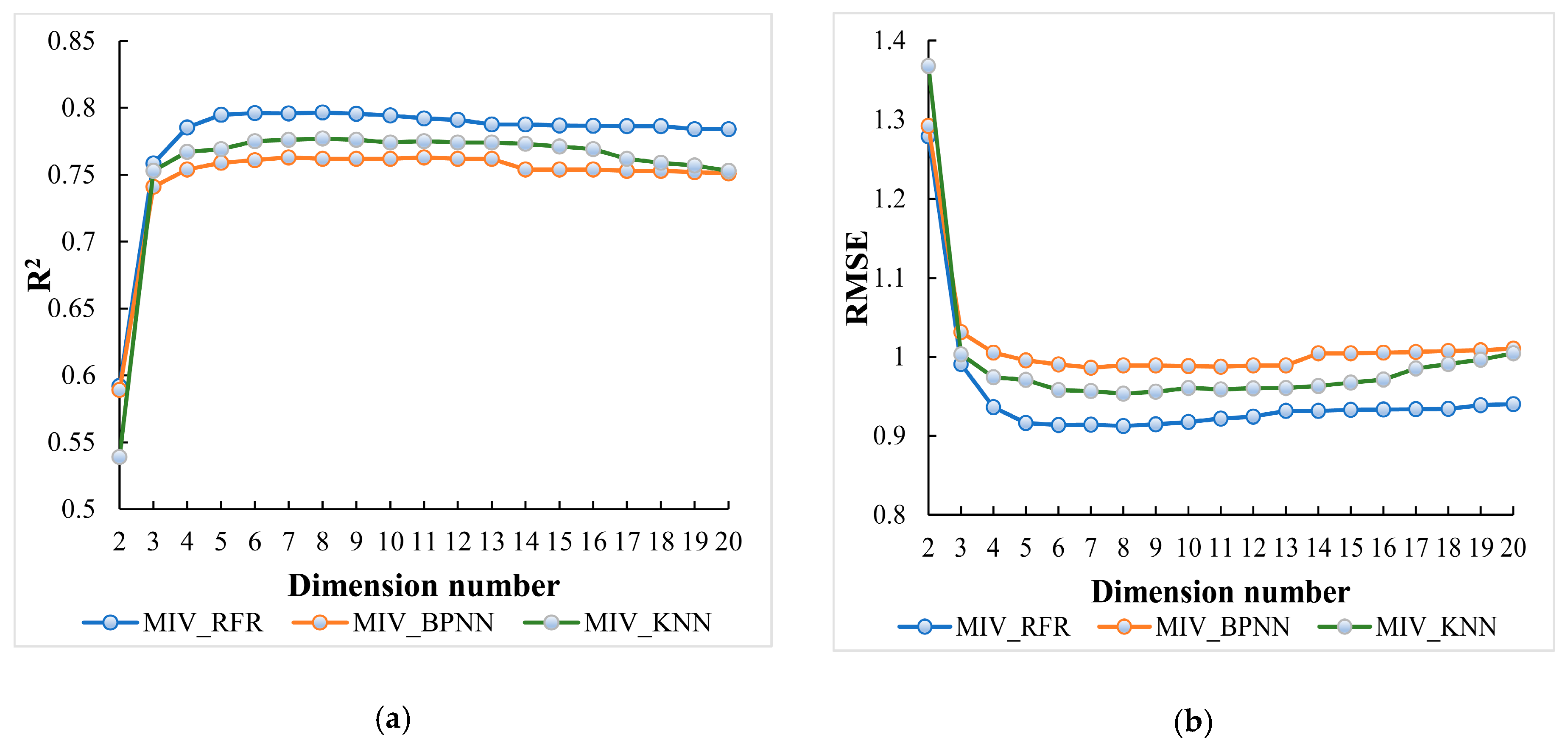
3.1. Determining the Dimension Number of the First FS Process

The nine models were derived using three FS methods (RF, MIV and K-means) and three ML algorithms (RFR, BPNN and KNN) in this study. The reason we chose these methods was that they represent different feature selection and regression criteria, which makes the LAI estimates more comparable. For example, although RF and MIV selection are both based on feature importance criteria, they rely on different ML algorithms. K-means is an unsupervised clustering algorithm that is only based on spectral similarity instead of the fixed regression method. Therefore, in theory, the features selected by K-means are not able to abide to one specific ML algorithm.

Different models show different RMSE trends with the changing of the input variable dimension (Figure 4). For example, the RMSE increased by 0.038 when the original data decreased to 10-dimension using the RF_RFR model. While the RMSE increased by 0.252, which is almost 7 times larger than the RF_RFR model when applying the RF_KNN model in the same dimensional condition. According to Figure 4, the changes in LAI estimation accuracy of all models can be divided into three categories: reducing continuously (MIV_KNN as category 1); decreasing sharply after a gradual change (RF_RFR, RF_KNN, RF_BPNN as category 2); increasing at initial and then decreasing (MIV_RFR, MIV_BPNN, K-means_RFR, K-means_KNN, K-means_BPNN as category 3). For category 2, the RMSE values only changed by 0.012, 0.008 and 0.015 along with the decreasing of dimension from 210 to 20. While with the dimension continuing to decrease (from 20 to 10), the RMSE values increased sharply by 0.026, 0.260 and 0.014. In addition, for category 3, the RMSE values continued to increase until the dimension reduced to 40 or 50 (depend on the models), then the RMSE started to decrease until the dimension decreased to 20. As the dimensions continue to decline, the LAI estimation accuracy reduced significantly. Therefore, 20 would be a suitable dimension number that maintains most information of the original data set while reduced nearly 90% redundant bands. Therefore, the complexity and computational efficiency of models would be improved obviously.

3.2. LAI Estimation Using Features Selected by the First FS Process

Table 4. LAI estimation accuracy of different machine learning methods.

FS	Machine Learning Method	Original Data Set		20 Dimensions
		R2	RMSE	R2	RMSE
RF	RFR	0.828	0.837	0.824	0.849
	KNN	0.764	0.982	0.768	0.974
	BPNN	0.797	0.910	0.791	0.925
MIV	RFR	0.828	0.837	0.784	0.940
	KNN	0.764	0.982	0.753	1.004
	BPNN	0.797	0.910	0.751	1.010
K-means	RFR	0.828	0.837	0.819	0.862
	KNN	0.764	0.982	0.751	1.008
	BPNN	0.797	0.910	0.793	0.921

shows the LAI estimation accuracy using different FS and ML algorithms. According to the accuracy indicators (R² and RMSE), RFR is the best ML algorithm with or without dimensionality reduction. When using original data set, RFR algorithm obtained higher estimation accuracy (with RMSE of 0.837) than KNN (with RMSE of 0.982) and BPNN (with RMSE of 0.910) algorithm. When the input variable dimension was reduced to 20, RFR still achieved the lowest RMSE values in each data set compared with other ML regression algorithms. In contrast, KNN achieved the lowest accuracy in all ML algorithms except MIV-based models.

Compared with MIV-selected and K-means-selected subsets (Table 4), using RF as feature selection generated the highest accuracy when using RFR and KNN. When using BPNN as the regression algorithm, the LAI estimation difference of the RF_BPNN and K-means_BPNN model could be neglected (with RMSE difference of 0.004). By contrast, those RMSE values of K-means-selected models (RMSE of 0.862, 1.008 and 0.921) and MIV-selected models (RMSE of 0.940, 1.004 and 1.010) were much larger than RF-selected models (RMSE of 0.849, 0.974 and 0.925). Therefore, the results indicate that the RF-selected data set retained more useful information of the original data set, while MIV selection discarded some important spectral bands that could reveal difference in estimation of LAI.

Therefore, RF shows excellent performance as both FS and regression methods, which proved the priority of RF among ML algorithms. Moreover, when using RF as the FS method, the RFR regression achieved the best estimation result. While the same FS and regression method combinations from MIV and BPNN have the worst LAI estimation accuracy among all the models, which indicates that using the same ML algorithm as the FS method cannot always guarantee the satisfactory LAI estimation accuracy.

To explain the reason why MIV-selected models achieve worse LAI estimation than other models, the selected bands of each FS method and their Pearson correlation coefficients are shown in

Table 5. First feature selection (FS) process selected bands using random forest (RF), mean impact value (MIV) and K-means methods.

Methods	Center Wavelength of Selected Bands of the Simulated Data and Its Corresponding Band Number of GF-5 Data
RF	502.5 nm (A1: Band27); 527.5 nm (A2: Band33); 672.5 nm (A3: Band67); 677.5 nm (A4: Band68); 723.5 nm (A5: Band78); 728.5 nm (A6: Band80); 732.5 nm (A7: Band81); 737.5 nm (A8: Band82); 741.5 nm (A9: Band83); 1055.5 nm (A10: Band157); 1067.5 nm (A11: Band158); 1080.5 nm (A12: Band160); 1089.5 nm (A13: Band161); 1097.5 nm (A14: Band162); 1105.5 nm (A15: Band163); 1114.5 nm (A16: Band164); 1266.5 nm (A17: Band182); 2007.5 nm (A18: Band270); 2209.5 nm (A19: Band294); 2428.5 nm (A20: Band320)
MIV	848.5 nm (B1: Band108); 877.5 nm (B2: Band115); 890.5 nm (B3: Band118); 937.5 nm (B4: Band129); 950.5 nm (B5: Band132); 967.5 nm (B6: Band136); 972.5 nm (B7: Band137); 1038.5 nm (B8: Band155); 1046.5 nm (B9: Band156); 1097.5 nm (B10: Band162); 1105.5 nm (B11: Band163); 1131.5 nm (B12: Band166); 1139.5 nm (B13: Band167); 1215.5 nm (B14: Band176); 1274.5 nm (B15: Band183); 1316.5 nm (B16: Band188); 1586.5 nm (B17: Band220); 1603.5 nm (B18: Band222); 1637.5 nm (B19: Band226); 1754.5 nm (B20: Band240)
K-means	502.5 nm (C1: Band27); 565.5 nm (C2: Band42); 612.5 nm (C3: Band53); 668.5 nm (C4: Band66); 702.5 nm (C5: Band74); 706.5 nm (C6: Band75); 711.5 nm (C7: Band76); 723.5 nm (C8: Band79); 728.5 nm (C9: Band80); 856.5 nm (C10: Band110); 886.5 nm (C11: Band117); 997.5 nm (C12: Band143); 1080.5 nm (C13: Band160); 1148.5 nm (C14: Band168); 1494.5 nm (C15: Band209); 1519.5 nm (C16: Band212); 1754.5 nm (C17: Band240); 2007.5 nm (C18: B270); 2260.5 nm (C19: Band300); 2319.5 nm (C20: Band307)

and Figure 5, respectively. Each variable in Figure 5 is corresponding to the bands in Table 5 with the same order. Bands selected by MIV were concentrated in the SWIR region with great linear correlation, which have limitations on the representation of canopy spectral information and lead to low LAI estimation accuracy. In contrast, bands selected by K-means and RF were well distributed in all regions (VIS, red-edge, NIR and SWIR), which also result in the high similarity of estimation results using K-means and RF selected data set.

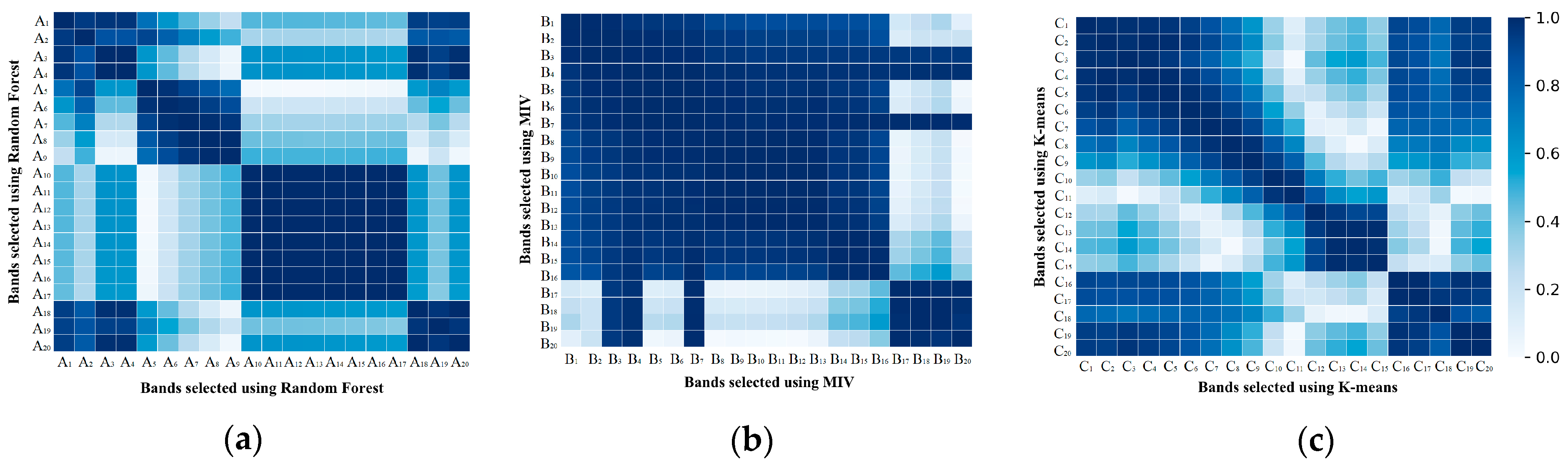
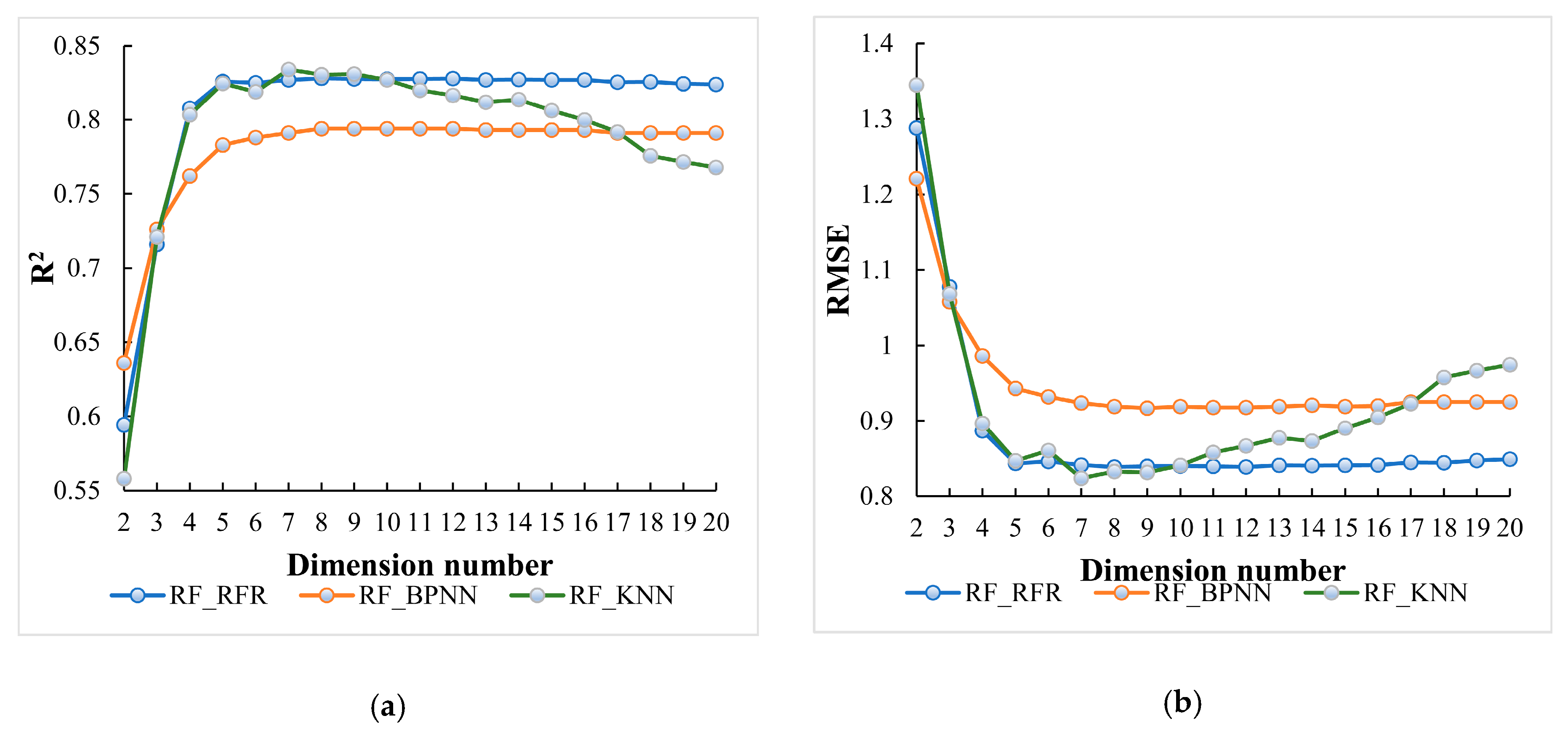
3.3. Optimal Bands Combination Searching in the Second FS Process

SBS is a heuristical search method to remove the bands that have a minimal impact on evaluating indicators. Figure 6 shows the performances of RF_RFR, RF_BPNN and RF_KNN models using SBS to search the optimal input variable data set for LAI estimation using GF-5 hyperspectral data. The results indicate that RFR and BPNN methods were robust with respect to the dimension number changing. When the dimension decreased from 20 to 8, the RMSE of RF_RFR and RF_BPNN decreased by 0.010 and 0.006, respectively. However, when the number of variables continued to decrease, the LAI estimation accuracy of those two models declined sharply. In contrast, the number of variables has a great influence on KNN. When the number decreased from 20 to 7, RMSE decreased by 0.151, which is almost 15 times larger than those of RF_RFR and RF_BPNN.

Figure 7 and Figure 8 show the performances of different ML methods using K-means and MIV as feature selection methods, respectively. RFR and BPNN methods were still robust to the input variable dimension changing. When using K-means as the FS method, RFR and BPNN achieved their highest LAI estimation accuracy when the input variables number decreased to 9 (RMSE of 0.809 and 0.906). While when using MIV as the FS method, RFR and BPNN achieved their highest LAI estimation accuracy when input variables number decreased to 8 and 11 (RMSE of 0.912 and 0.987).

However, the trend of LAI estimation accuracy by KNN is related to input variables selected by different FS methods. For instance, Figure 7 shows that RMSE of RF_KNN decreased by 0.026 when the number of input variables decreased from 20 to 14, and then the accuracy dropped significantly with the decrease of the input variables dimension. While using MIV as the FS method, KNN shows good stability like RFR and BPNN.

Table 6. Best LAI estimation accuracy of each FS and ML method combination.

FS	ML Method	R2	RMSE	Number of Input Variables	Center Wavelength of the Selected Bands
RF	RFR	0.828	0.839	8	502.5 nm; 527.5 nm; 677.5 nm; 1055.5 nm; 1080.5 nm; 1097.5 nm; 1266.5 nm; 2428.5 nm
	BPNN	0.794	0.919	8	502.5 nm; 527.5 nm; 672.5 nm; 728.5 nm; 1080.5 nm; 2007.5 nm; 2209.5 nm; 2428.5 nm
	KNN	0.834	0.824	7	502.5 nm; 677.5 nm; 1114.5 nm; 1266.5 nm; 2007.5 nm; 2209.5 nm; 2428.5 nm
K-means	RFR	0.840	0.809	9	502.5 nm; 612.5 nm; 723.5 nm; 856.5 nm; 997.5 nm; 1148.5 nm; 1519.5 nm; 1754.5 nm; 2319.5 nm
	BPNN	0.799	0.906	9	502.5 nm; 565.5 nm; 668.5 nm; 702.5 nm; 723.5 nm; 856.5 nm; 1080.5 nm; 1519.5 nm; 2260.5 nm;
	KNN	0.764	0.982	14	502.5 nm; 612.5 nm; 702.5 nm; 706.5 nm; 711.5 nm; 723.5 nm; 728.5 nm; 1080.5 nm; 1148.5 nm; 1494.5 nm; 1519.5 nm; 1754.5 nm; 2260.5 nm; 2319.5 nm
MIV	RFR	0.796	0.912	8	877.5 nm; 890.5 nm; 972.5 nm; 950.5 nm; 1046.5 nm; 1097.5 nm; 1215.5 nm; 1274.5 nm;
	BPNN	0.763	0.987	11	967.5 nm; 972.5 nm; 1038.5 nm; 1046.5 nm; 1097.5 nm; 1131.5 nm; 1139.5 nm; 1215.5 nm; 1274.5 nm; 1316.5 nm; 1637.5 nm;
	KNN	0.777	0.953	8	967.5 nm; 972.5 nm; 1097.5 nm; 1105.5 nm; 1139.5 nm; 1215.5 nm; 1274.5 nm; 1316.5 nm

shows the best performance of each FS and ML method combination. According to Table 4, Table 6 and Figure 6a, the bands distributed in RE and NIR (<1100 nm) had a negative effect on the LAI estimation accuracy of the RF_KNN model. Removing those bands significantly improved the LAI estimation accuracy. However, the RE bands are indispensable to maintain the LAI estimation accuracy of the K-means_KNN model since the RMSE will at least increase by 0.132 if the dimension changed from 14 to 13. On the other hand, although RF_RFR and RF_KNN models achieved similar LAI estimation accuracy, their final selected bands were distributed differently.

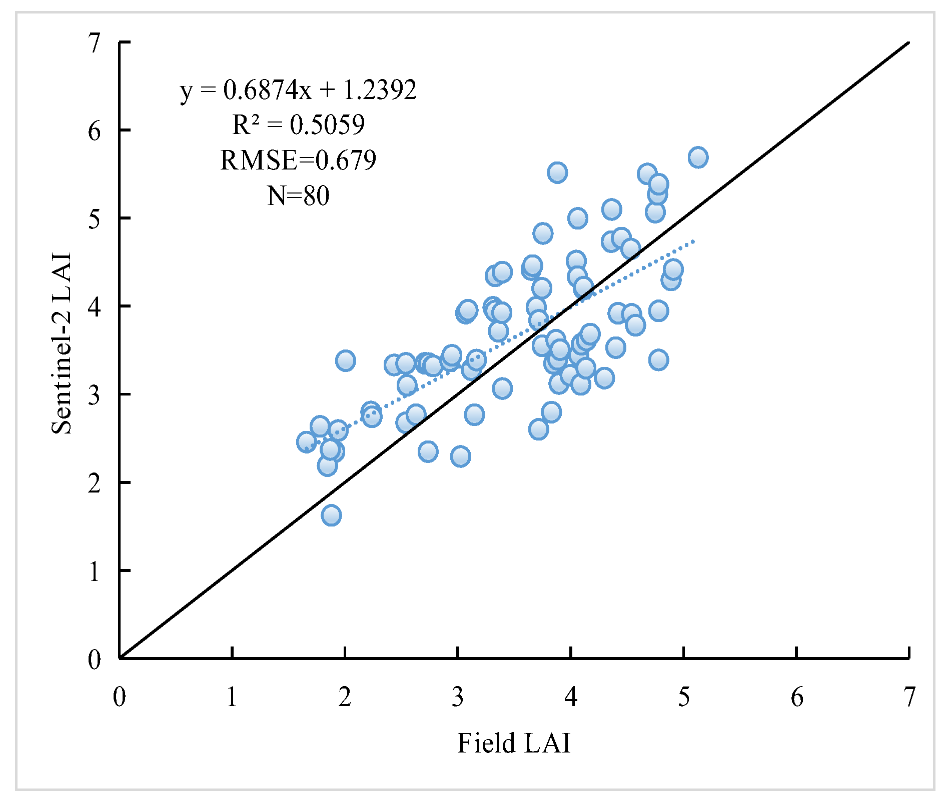
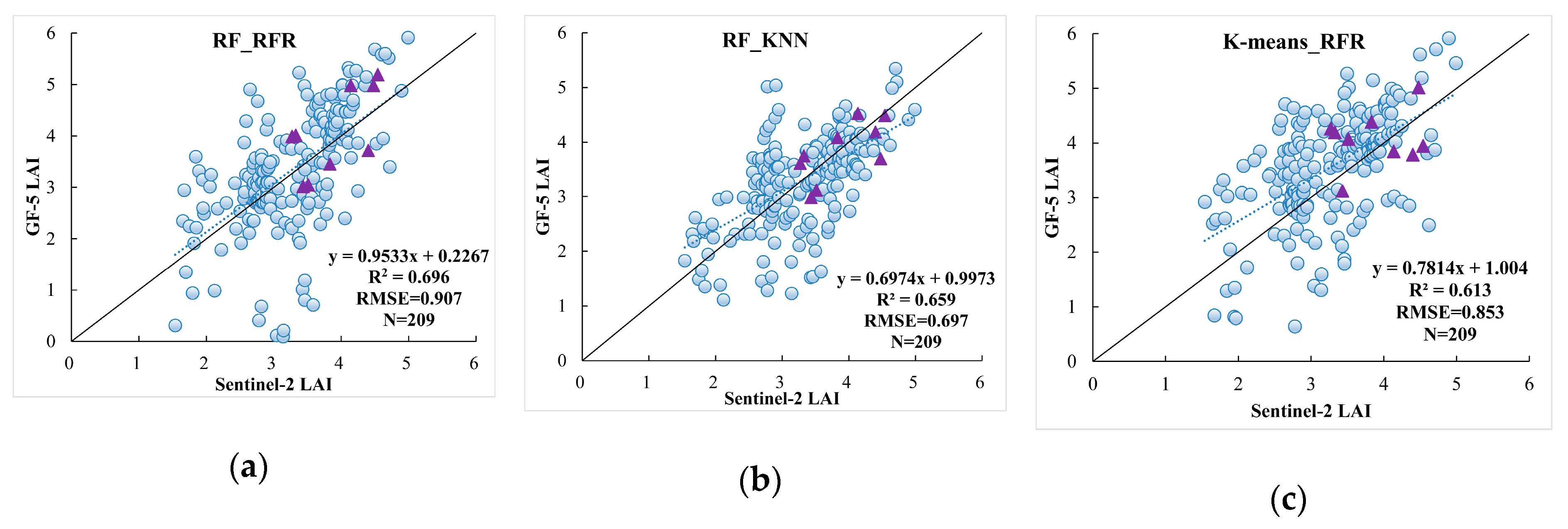
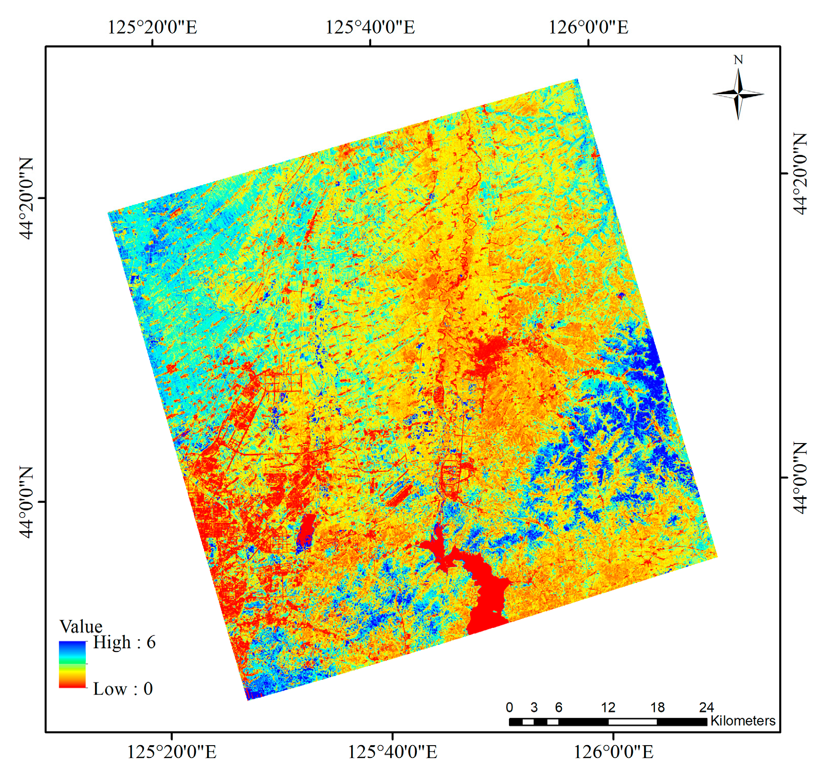
3.4. Evaluation of GF-5 LAI Estimation

According to Table 6, there are only three models with RMSE less than 0.85. Therefore, RF_RFR, RF_KNN and K-means_RFR models were selected to access the LAI estimation accuracy using actual GF-5 hyperspectral data (Figure 9). RF_RFR model had the highest R², but its RMSE value was the largest one among all the LAI estimation results. In addition, some low LAI estimates present in the reference value range of 2–4 when using the RF_RFR model. K-means_RFR shows an overestimation in the range of 2–5, whereas the LAI estimates from RF_KNN achieved the best performance (R² = 0.659, RMSE = 0.697). In Figure 9, the purple triangles represent the filed-measured LAI points. Similarly, RF_RFR and K-means_RFR models still show greater overestimation than the RF_KNN model.

Figure 10 shows the LAI estimation results using the 7-band RF_KNN model. According to the land-use map (FROM-GLC30) [82] shown in Figure 2, the LAI estimations of the RF_KNN model conform to the distribution characteristics of different land cover types. For instant, the forest region, which was mostly located in the southeast of Figure 2, had high LAI estimations ranging from 5 to 6. In the northwest is the corn filed (classified as cropland in Figure 2), which also had high LAI estimations ranging from 3 to 6. There are also some fallow land and vegetable filed regions (also classified as cropland in Figure 2) located in the northeast and southeast, they had low LAI estimations ranging from 0 to 3. The red regions in Figure 10, which had LAI estimations close to 0, were the impervious surfaces and water bodies. In general, the 7 band RF_KNN model is suitable for LAI estimation using GF-5 hyperspectral data.

4. Discussion

This study proposed a LAI estimation algorithm for GF-5 hyperspectral data based on the PROSAIL model as well as different feature selection and machine learning methods. The PROSAIL model can simulate extensive vegetation and underlying surface situations, which result in wide applicability of the proposed LAI estimation method. This LAI estimation method can be operated without any prior knowledge, it is also robust to the vegetation type and soil background. The seven selected spectral bands of the RF_KNN model maintain most information of the original hyperspectral data, which have achieved satisfactory LAI estimation accuracy validated by both simulated data and actual GF-5 data. This LAI estimation model developing method through comparison of different feature selection and machine learning methods is also suitable for other biophysical parameters inversion method development using hyperspectral data, such as FVC, fraction of absorbed photosynthetically active radiation (FPAR) and chlorophyll content.

Compared with multispectral data, hyperspectral data contains much more detailed information about reflectance properties of vegetation canopies. The effects of those abundant spectral bands in LAI estimation are always been discussed. For example, Lee et al. [83] confirmed the advantage of those abundant bands by comparing the LAI estimation accuracies of AVIRS and Landsat ETM+ data. Similarly, the research conducted by Das et al. [84] also indicated that Hyperion hyperspectral bands performed better than Landsat-8 and Sentinel-2 data in LAI estimation. The board-band reflectance and VIs show occurrence of saturation in high amounts of biomass, therefore they usually underestimate LAI in the high value region [85,86]. In contrast, the narrow-band VIs [28,29,87] are more sensitive to biomass change than board-band VIs, therefore those valuable variables, which provided by hyperspectral data contribute to achieve higher estimation accuracy in the high LAI value region [88,89]. Moreover, the advantages of higher spectral resolution and narrow-band VIs give hyperspectral data abilities in distinguishing vegetation types, thus the LAI could be estimated more accurately according to the different classification categories [90].

In general, the statistical regression methods applied in LAI estimation mainly based on the multiple-linear model with spectral bands or VIs as inputs [91,92,93]. However, it is difficult to describe the relationship between those independent variables and LAI using linear models. In contrast, the machine learning algorithms have excellent performances on establishing the nonlinear relationship between the dependent and independent variables [94,95]. Furthermore, traditional statistical regression methods are more sensitive to the multicollinearity between independent variables [96,97]. Although principal component regression (PCR) and partial least squared regression (PLSR) can improve the LAI estimation accuracy, some studies indicated that they still achieved lower accuracy than ML regression algorithms [98,99,100].

Table 7. LAI estimation performances using the partial least squared regression (PLSR) algorithm based on different data sets.

Data Set	Simulated Data		GF-5 Data		Optimal Number of Components
	R2	RMSE	R2	RMSE
RF-based (20 bands)	0.822	0.841	0.547	1.168	3
MIV-based (20 bands)	0.791	0.918	0.523	1.346	2
K-means-based (20 bands)	0.809	0.922	0.528	1.199	3

shows the best LAI estimation accuracy using the PLSR algorithm based on different data sets selected by RF, MIV and K-means algorithms in this study. Those best LAI estimates generated by PLSR algorithms have higher RMSEs than ML-based methods, especially for the GF-5 data. Those results confirm the previous research [98,99,100] by revealing the low robustness to noise of the PLSR algorithm. Therefore, ML algorithms still will be considered as a better choice for LAI (and other biophysical parameters) estimation.

The applications of ML regression methods to hyperspectral data processing in the field of quantitative remote sensing are developed rapidly [39,101]. However, the collinear relationship between adjacent bands hampers the vegetation parameter estimation accuracy. Most previous studies on LAI estimation employing the hybrid model and some vegetation indices (VIs) from hyperspectral data were preferred to be used to avert dimensionality curse [92,93,102]. Although VIs have great linear or nonlinear relationships with LAI in some cases, they only represent a small part of hyperspectral reflectance information. This study focused on searching the most representative input variables by investigating all the hyperspectral reflectance. It not only avoids the subjectivity of input variable selection for LAI estimation, but also makes full use of the advantage of hyperspectral bands. Furthermore, feature selection algorithms usually applied only once in most studies [39,103,104], such as choosing variables according to importance scores. However, most of the scores only represent the correlation between one specific input variable and the LAI. Therefore, it does not guarantee that the combination of high scored variables would be the optimal choice for LAI estimation. The two-step FS process confirmed this hypothesis by showing more accurate estimations using only a small part of the variables. Those RF-based and MIV-based models (selected by important score ranking) achieved better performances after the optimal variables searching strategy conducted by the SBS algorithm. Therefore, this two-step FS process has been proven to be suitable for LAI estimation.

Due to the limitation of available GF-5 hyperspectral data, the performance of the proposed algorithm was verified by reference LAI, which including field measured LAI and Sentinel-2 data derived LAI. According to the error transmission theory, the Sentinel-2 data derived LAI values have some influence on accuracy validation of LAI estimation from GF-5 data. Therefore, more field experiments are needed to conduct in the further to access the accuracy of this GF-5 LAI estimation algorithm.

5. Conclusions

In this study, a LAI estimation algorithm for GF-5 hyperspectral reflectance base on different FS and ML methods was proposed. According to the performances presented in this study, GF-5 hyperspectral reflectance data achieved satisfactory LAI estimations with R² of 0.659 and RMSE of 0.697 using a RF_KNN model (7 bands). The main conclusions are as follows:

(1)

Using the same ML algorithm as feature selection and regression methods could not always ensure an optimal LAI estimation result. In this study, the RF_RFR model using the random forest algorithm as both FS and regression methods achieved higher estimation accuracy than RF_BPNN and RF_KNN when using simulated data. The MIV_BPNN is another model that uses the same algorithm as the FS and regression method. However, this model yielded lower estimation accuracy than using other regression algorithms (MIV_RFR and MIV_KNN).

(2)

The RF algorithm can be regarded as one of the most adaptable algorithms for further studies of biophysical parameters estimation using hyperspectral data. Not only RF-based features retained the most useful information for LAI estimation, but this algorithm was also less affected by the redundant variables when used as the regression method.

(3)

The proposed two-step feature selection process can achieve more satisfactory estimations with even fewer inputs. The study indicates that the feature ranking provided by RF and MIV only represents the importance of a single feature, thus the combination of high-score features could not represent the best inputs of the LAI estimation model. While the additional selection process based on the SBS algorithm was very effective in the optimal subset searching in a small or moderate dimension. Therefore, this two-step feature selection method improved the model performance by taking advantage of two FS algorithms with different criteria (first to reduce dimension, then search for the optimal subset). This proposed method was not only suitable for LAI estimation, but also can be used for classification based on hyperspectral remote sensing data.

The approach provided in this study assessed the application of GF-5 reflectance data in LAI estimation. Further research will focus on developing some effective narrow-band vegetation indexes for biophysical parameters estimation using GF-5 data.

References

1. Chen, J.M.; Pavlic, G.; Brown, L.; Cihlar, J.; Leblanc, S.G.; White, H.P.; Hall, R.J.; Peddle, D.R.; King, D.J.; Trofymow, J.A.; et al. Derivation and validation of canada-wide coarse-resolution leaf area index maps using high-resolution satellite imagery and ground measurements. Remote Sens. Environ. 2002, 80, 165–184. [Google Scholar] [CrossRef]
2. Karimi, S.; Sadraddini, A.A.; Nazemi, A.H.; Xu, T.; Fard, A.F. Generalizability of gene expression programming and random forest methodologies in estimating cropland and grassland leaf area index. Comput. Electron. Agric. 2018, 144, 232–240. [Google Scholar] [CrossRef]
3. Wang, L.; Wang, P.; Liang, S.; Qi, X.; Li, L.; Xu, L. Monitoring maize growth conditions by training a bp neural network with remotely sensed vegetation temperature condition index and leaf area index. Comput. Electron. Agric. 2019, 160, 82–90. [Google Scholar] [CrossRef]
4. Calders, K.; Origo, N.; Disney, M.; Nightingale, J.; Woodgate, W.; Armston, J.; Lewis, P. Variability and bias in active and passive ground-based measurements of effective plant, wood and leaf area index. Agric. For. Meteorol. 2018, 252, 231–240. [Google Scholar] [CrossRef]
5. Hales, K.; Neelin, J.D.; Zeng, N. Sensitivity of tropical land climate to leaf area index: Role of surface conductance versus albedo. J. Clim. 2004, 17, 1459–1473. [Google Scholar] [CrossRef]
6. Gonsamo, A.; Walter, J.M.; Chen, J.M.; Pellikka, P.; Schleppi, P. A robust leaf area index algorithm accounting for the expected errors in gap fraction observations. Agric. For. Meteorol. 2018, 248, 197–204. [Google Scholar] [CrossRef]
7. Xiao, Z.; Liang, S.; Jiang, B. Evaluation of four long time-series global leaf area index products. Agric. For. Meteorol. 2017, 246, 218–230. [Google Scholar] [CrossRef]
8. Delegido, J.; Verrelst, J.; Meza, C.M.; Rivera, J.P.; Alonso, L.; Moreno, J. A red-edge spectral index for remote sensing estimation of green LAI over agroecosystems. Eur. J. Agron. 2013, 46, 42–52. [Google Scholar] [CrossRef]
9. Zhu, X.; Skidmore, A.K.; Wang, T.; Liu, J.; Darvishzadeh, R.; Shi, Y.; Premier, J.; Heurich, M. Improving leaf area index (LAI) estimation by correcting for clumping and woody effects using terrestrial laser scanning. Agric. For. Meteorol. 2018, 263, 276–286. [Google Scholar] [CrossRef]
10. Soudani, K.; François, C.; Le Maire, G.; Le Dantec, V.; Dufrêne, E. Comparative analysis of IKONOS, SPOT, and ETM+ data for leaf area index estimation in temperate coniferous and deciduous forest stands. Remote Sens. Environ. 2006, 102, 161–175. [Google Scholar] [CrossRef] [Green Version]
11. Xiao, Z.; Liang, S.; Wang, J.; Chen, P. Use of general regression neural networks for generating the glass leaf area index product from time-series MODIS surface reflectance. IEEE Trans. Geosci. Remote Sens. 2014, 52, 209–223. [Google Scholar] [CrossRef]
12. Huang, D.; Knyazikhin, Y.; Wang, W.; Deering, D.W.; Stenberg, P.; Shabanov, N.; Tan, B.; Myneni, R.B. Stochastic transport theory for investigating the three-dimensional canopy structure from space measurements. Remote Sens. Environ. 2008, 112, 35–50. [Google Scholar] [CrossRef]
13. Xie, Y.; Wang, P.; Bai, X.; Khan, J.; Zhang, S.; Li, L.; Wang, L. Assimilation of the leaf area index and vegetation temperature condition index for winter wheat yield estimation using Landsat imagery and the CERES-Wheat model. Agric. For. Meteorol. 2017, 246, 194–206. [Google Scholar] [CrossRef]
14. Ganguly, S.; Nemani, R.R.; Zhang, G.; Hashimoto, H.; Milesi, C.; Michaelis, A.; Wang, W.; Votava, P.; Samanta, A.; Melton, F.; et al. Generating global Leaf Area Index from Landsat: Algorithm formulation and demonstration. Remote Sens. Environ. 2012, 122, 185–202. [Google Scholar] [CrossRef] [Green Version]
15. Wang, J.; Xiao, X.M.; Bajgain, R.; Starks, P.; Steiner, J.; Doughty, R.B.; Chang, Q. Estimating leaf area index and aboveground biomass of grazing pastures using Sentinel-1, Sentinel-2 and Landsat images. ISPRS J. Photogramm. Remote Sens. 2019, 154, 189–201. [Google Scholar] [CrossRef] [Green Version]
16. Li, W.; Niu, Z.; Wang, C.; Huang, W.; Chen, H.; Gao, S.; Li, D.; Muhammad, S. Combined use of airborne Lidar and satellite GF-1 data to estimate leaf area index, height, and aboveground biomass of maize during peak growing season. IEEE J. Sel. Top. Appl. Earth Obs. Remote Sens. 2015, 8, 4489–4501. [Google Scholar] [CrossRef]
17. Wei, X.; Gu, X.; Meng, Q.; Yu, T.; Zhou, X.; Wei, Z.; Jia, K.; Wang, C. Leaf Area Index Estimation Using Chinese GF-1 Wide Field View Data in an Agriculture Region. Sensors 2017, 17, 1593. [Google Scholar] [CrossRef] [PubMed]
18. Asner, G.P.; Martin, R.E. Airborne spectranomics: Mapping canopy chemical and taxonomic diversity in tropical forests. Front. Ecol. Environ. 2009, 7, 269–276. [Google Scholar] [CrossRef] [Green Version]
19. Thenkabail, P.S.; Smith, R.B.; Pauw, E.D. Hyperspectral vegetation indices and their relationships with agricultural crop characteristics. Remote Sens. Environ. 2000, 71, 158–182. [Google Scholar] [CrossRef]
20. Perry, E.M.; Davenport, J.R. Spectral and spatial differences in response of vegetation indices to nitrogen treatments on apple. Comput. Electron. Agric. 2007, 59, 56–65. [Google Scholar] [CrossRef]
21. Luo, S.; Wang, C.; Xi, X.; Pan, F.; Qian, M.; Peng, D.; Nie, S.; Qin, H.; Lin, Y. Retrieving aboveground biomass of wetland Phragmites australis (common reed) using a combination of airborne discrete-return LiDAR and hyperspectral data. Int. J. Appl. Earth Obs. Geoinf. 2017, 58, 107–117. [Google Scholar] [CrossRef]
22. Ustin, S.L.; Roberts, D.A.; Gamon, J.A.; Asner, G.P.; Green, R.O. Using imaging spectroscopy to study ecosystem processes and properties. Bioscience 2004, 54, 523–534. [Google Scholar] [CrossRef]
23. Smith, M.L.; Ollinger, S.V.; Martin, M.E.; Aber, J.D.; Goodale, H.C.L. Direct estimation of aboveground forest productivity through hyperspectral remote sensing of canopy nitrogen. Ecol. Appl. 2002, 12, 1286–1302. [Google Scholar] [CrossRef]
24. Li, X.; Zhang, Y.; Bao, Y.; Luo, J.; Jin, X.; Xu, X.; Song, X.; Yang, G. Exploring the best hyperspectral features for LAI estimation using partial least squares regression. Remote Sens 2014, 6, 6221–6241. [Google Scholar] [CrossRef] [Green Version]
25. Meroni, M.; Colombo, R.; Panigada, C. Inversion of a radiative transfer model with hyperspectral observations for LAI mapping in poplar plantations. Remote Sens. Environ. 2004, 92, 195–206. [Google Scholar] [CrossRef]
26. Zhang, X.; Liao, C.; Li, J.; Sun, Q. Fractional vegetation cover estimation in arid and semi-arid environments using hj-1 satellite hyperspectral data. Int. J. Appl. Earth Obs. Geoinf. 2013, 21, 506–512. [Google Scholar] [CrossRef]
27. Jiao, Q.; Zhang, B.; Liu, J.; Liu, L. A novel two-step method for winter wheat-leaf chlorophyll content estimation using hyperspectral vegetation index. Int. J. Remote Sens. 2014, 35, 7363–7375. [Google Scholar] [CrossRef]
28. Kanning, M.; Kühling, I.; Trautz, D.; Jarmer, T. High-Resolution UAV-Based Hyperspectral Imagery for LAI and Chlorophyll Estimations from Wheat for Yield Prediction. Remote Sens. 2018, 10, 2000. [Google Scholar] [CrossRef] [Green Version]
29. George, R.; Padalia, H.; Sinha, S.K.; Kumar, A.S. Evaluation of the use of hyperspectral vegetation indices for estimating mangrove leaf area index in middle Andaman Island, India. Remote Sens. Lett. 2018, 9, 1099–1108. [Google Scholar] [CrossRef]
30. Feng, J.; Jiao, L.; Liu, F.; Sun, T.; Zhang, X. Unsupervised feature selection based on maximum information and minimum redundancy for hyperspectral images. Pattern Recognit. 2015, 51, 295–309. [Google Scholar] [CrossRef]
31. Taskin, G.; Kaya, H.; Bruzzone, L. Feature selection based on high dimensional model representation for hyperspectral images. IEEE Trans. Image Process. 2017, 26, 2918–2928. [Google Scholar] [CrossRef] [PubMed]
32. Majdi, M.M.; Seyedali, M. Whale Optimization Approaches for Wrapper Feature Selection. Appl. Soft Comput. 2017, 62, 441–453. [Google Scholar]
33. Samsudin, S.H.; Shafri, H.Z.M.; Hamedianfar, A.; Mansor, S. Spectral feature selection and classification of roofing materials using field spectroscopy data. J. Appl. Remote Sens. 2015, 9, 95079. [Google Scholar] [CrossRef]
34. Kumar, A.; Patidar, V.; Khazanchi, D.; Saini, P. Optimizing feature selection using particle swarm optimization and utilizing ventral sides of leaves for plant leaf classification. Procedia Comput. Sci. 2016, 89, 324–332. [Google Scholar] [CrossRef] [Green Version]
35. Khaled, A.Y.; Aziz, S.A.; Bejo, S.K.; Nawi, N.M.; Jamaludin, D.; Ibrahim, N.U.A. A comparative study on dimensionality reduction of dielectric spectral data for the classification of basal setm rot (BSR) disease in oil palm. Comput. Electron. Agric. 2020, 170, 105288. [Google Scholar] [CrossRef]
36. Lee, J.A.; Verleysen, M. Nonlinear dimensionality reduction of data manifolds with essential loops. Neurocomputing 2005, 67, 29–53. [Google Scholar] [CrossRef]
37. Alvarez-Meza, A.M.; Lee, J.A.; Verleysen, M.; Castellanos-Dominguez, G. Kernel-based dimensionality reduction using Renyi’s α-entropy measures of similarity. Neurocomputing 2017, 222, 36–46. [Google Scholar] [CrossRef]
38. Chen, Y.; Wu, X.; Li, T.; Cheng, J.; Ou, Y.; Xu, M. Dimensionality reduction of data sequences for human activity recognition. Neurocomputing 2016, 210, 294–302. [Google Scholar] [CrossRef]
39. Rivera-Caicedo, J.P.; Verrelst, J.; Muñoz-Marí, J.; Camps-Valls, G.; Moreno, J. Hyperspectral dimensionality reduction for biophysical variable statistical retrieval. ISPRS J. Photogramm. Remote Sens. 2017, 132, 88–101. [Google Scholar] [CrossRef]
40. Chan, K.Y.; Aydin, M.E.; Fogarty, T.C. Main effect fine-tuning of the mutation operator and the neighbourhood function for uncapacitated facility location problems. Soft Comput. 2006, 10, 1075–1090. [Google Scholar] [CrossRef]
41. Imani, M.B.; Pourhabibi, T.; Keyvanpour, M.R.; Azmi, R. A new feature selection method based on ant colony and genetic algorithm on persian font recognition. Int. J. Mach. Learn. Comput. 2012, 2, 278–282. [Google Scholar] [CrossRef]
42. Karegowda, A.G.; Manjunath, A.S.; Jayaram, M.A. Comparative study of attribute selection using gain ratio and correlation-based feature selection. Int. J. Inf. Technol. Knowl. Manag. 2010, 2, 271–277. [Google Scholar]
43. Sylvester, E.V.; Bentzen, P.; Bradbury, I.R.; Clément, M.; Pearce, J.; Horne, J.; Beiko, R.G. Applications of random forest feature selection for fine-scale genetic population assignment. Evolut. Appl. 2018, 11, 153–165. [Google Scholar] [CrossRef] [PubMed]
44. Lee, C.P.; Lin, C.J. Large-scale linear ranksvm. Neural Comput. 2014, 26, 781–817. [Google Scholar] [CrossRef] [Green Version]
45. Lan, L.; Wang, Z.; Zhe, S.; Cheng, W.; Wang, J.; Zhang, K. Scaling up kernel SVM on limited resources: A low-rank linearization approach. IEEE Trans. Neural Netw. Learn. Syst. 2019, 30, 369–378. [Google Scholar] [CrossRef] [Green Version]
46. Joachims, T. Making large-scale svm learning practical. Tech. Rep. 1998, 8, 499–526. [Google Scholar]
47. Berger, K.; Atzberger, C.; Danner, M.; D’Urso, G.; Mauser, W.; Vuolo, F.; Hank, T. Evaluation of the PROSAIL model capabilities for future hyperspectral model environments: A review study. Remote Sens. 2018, 10, 85. [Google Scholar] [CrossRef] [Green Version]
48. Darvishzadeh, R.; Skidmore, A.; Abdullah, H.; Cherenet, E.; Ali, A.; Wang, T.; Nieuwenhuis, W.; Heurich, M.; Vrieling, A.; O’Connor, B.; et al. Mapping leaf chlorophyll content from Sentinel-2 and RapidEye data in spruce stands using the invertible forest reflectance model. Int. J. Appl. Earth Obs. Geoinf. 2019, 79, 58–70. [Google Scholar] [CrossRef] [Green Version]
49. Poursanidis, D.; Traganos, D.; Reinartz, P.; Chrysoulakis, N. On the use of Sentinel-2 for coastal habitat mapping and satellite-derived bathymetry estimation using downscaled coastal aerosol band. Int. J. Appl. Earth Obs. Geoinf. 2019, 80, 58–70. [Google Scholar] [CrossRef]
50. Xie, Q.; Dash, J.; Huete, A.; Jiang, A.; Yin, G.; Ding, Y.; Peng, D.; Hall, C.C.; Brown, L.; Shi, Y.; et al. Retrieval of crop biophysical parameters from Sentinel-2 remote sensing imagery. Int. J. Appl. Earth Obs. Geoinf. 2019, 80, 187–195. [Google Scholar] [CrossRef]
51. Pasqualotto, N.; Delegido, J.; Wittenberghe, S.A.; Rinaldi, M.; Moreno, J. Multi-Crop green LAI estimation with a new simple Sentinel-2 LAI index. Sensors 2019, 19, 904. [Google Scholar] [CrossRef] [PubMed] [Green Version]
52. Mbulisi, S.; Onisimo, M.; Timothy, D.; Thulile, S.V.; Paramu, L.M. Estimating LAI and mapping canopy storage capacity for hydrological applications in wattle infested ecosystems using Sentinel-2 MSI derived red edge bands. Gisci. Remote Sens. 2019, 56, 68–86. [Google Scholar]
53. Pearlman, J.S.; Barry, P.S.; Segal, C.C.; Shepanski, J.; Carman, S.L. Hyperion, a space-based imaging spectrometer. IEEE Trans. Geosci. Remote Sens. 2003, 41, 1160–1173. [Google Scholar] [CrossRef]
54. Datt, B.; Mcvicar, T.R.; Van Niel, T.G.; Jupp, D.L.B.; Pearlman, J.S. Preprocessing eo-1 hyperion hyperspectral data to support the application of agricultural indexes. IEEE Trans. Geosci. Remote Sens. 2003, 41, 1246–1259. [Google Scholar] [CrossRef] [Green Version]
55. Jacquemoud, S.; Verhoef, W.; Baret, F.; Bacour, C.; Zarco-Tejada, P.J.; Asner, G.P.; François, C.; Ustin, S.L. PROSPECT+ SAIL models: A review of use for vegetation characterization. Remote Sens. Environ. 2009, 113, 56–66. [Google Scholar] [CrossRef]
56. Atzberger, C.; Richter, K. Spatially constrained inversion of radiative transfer models for improved LAI mapping from future sentinel-2 imagery. Remote Sens. Environ. 2012, 120, 208–218. [Google Scholar] [CrossRef]
57. Wang, B.; Jia, K.; Liang, S.; Xie, X.; Wei, X.; Zhao, X.; Yao, Y.; Zhang, X. Assessment of Sentinel-2 MSI spectral band reflectance for estimating fractional vegetation cover. Remote Sens. 2018, 10, 1927. [Google Scholar] [CrossRef] [Green Version]
58. Tao, G.; Jia, K.; Zhao, X.; Wei, X.; Xie, X.; Zhang, X.; Wang, B.; Yao, Y.; Zhang, X. Generating high spatio-temporal resolution fractional vegetation cover by fusing GF-1 WFV and MOSID data. Remote Sens. 2019, 11, 2324. [Google Scholar] [CrossRef] [Green Version]
59. Weiss, M.; Baret, F.; Smith, G.J.; Jonckheere, I.; Coppin, P. Review of methods for in situ leaf area index (LAI) determination: Part II. Estimation of LAI, errors and sampling. Agric. For. Meteorol. 2004, 121, 37–53. [Google Scholar] [CrossRef]
60. Baret, F.; Hagolle, O.; Geiger, B.; Bicheron, P.; Miras, B.; Huc, M.; Berthelot, B.; Niño, F.; Weiss, M.; Samain, O.; et al. Lai, fapar and fcover cyclopes global products derived from vegetation: Part 1: Principles of the algorithm. Remote Sens. Environ. 2007, 110, 275–286. [Google Scholar] [CrossRef] [Green Version]
61. Ho, T.K. The random subspace method for constructing decision forests. IEEE Trans. Pattern Anal. Mach. Intell. 1998, 20, 832–844. [Google Scholar]
62. Genuer, R.; Poggi, J.M.; Tuleau-Malot, C. Variable selection using random forests. Pattern Recognit. Lett. 2010, 31, 2225–2236. [Google Scholar] [CrossRef] [Green Version]
63. Ou, Q.; Lei, X.; Shen, C. Individual tree diameter growth models of Larch-Spruce-Fir mixed forests based on machine learning algorithm. Forests 2019, 10, 187. [Google Scholar] [CrossRef] [Green Version]
64. Rahman, M.M.; Zhang, X.; Ahmed, I.; Iqbal, Z.; Zeraatpisheh, M.; Kanzaki, M.; Xu, M. Remote sensing-based mapping of senescent leaf C:N ratio in the sundarbans reserved forest using machine learning techniques. Remote Sens. 2020, 12, 1375. [Google Scholar] [CrossRef]
65. Qi, M.; Fu, Z.; Chen, F. Research on a feature selection method based on median impact value for modeling in thermal power plants. Appl. Therm. Eng. 2016, 94, 472–477. [Google Scholar] [CrossRef]
66. Tan, X.; Ji, Z.; Zhang, Y. Non-invasive continuous blood pressure measurement based on mean impact value method, bp neural network, and genetic algorithm. Technol. Health Care 2018, 26, 1–15. [Google Scholar] [CrossRef] [Green Version]
67. Kanungo, T.; Mount, D.M.; Netanyahu, N.S.; Piatko, C.D.; Silverman, R.; Wu, A.Y. An efficient k-means clustering algorithm: Analysis and implementation. IEEE Trans. Pattern Anal. Mach. Intell. 2002, 24, 881–892. [Google Scholar] [CrossRef]
68. Zhou, Q.; Zhao, Y. The design and implementation of intrusion detection system based on data mining technology. Res. J. Appl. Sci. Eng. Technol. 2013, 5, 204–208. [Google Scholar] [CrossRef]
69. Manju, V.N.; Lenin Fred, A. Ac coefficient and k-means cuckoo optimisation algorithm-based segmentation and compression of compound images. IET Image Process. 2018, 12, 218–225. [Google Scholar] [CrossRef]
70. Breiman, L. Random forests. Mach. Learn. 2001, 45, 5–32. [Google Scholar] [CrossRef] [Green Version]
71. Vigneau, E.; Courcoux, P.; Symoneaux, R.; Guérin, L.; Villière, A. Random forests: A machine learning methodology to highlight the volatile organic compounds involved in olfactory perception. Food Q. Prefer. 2018, 68, 135–145. [Google Scholar] [CrossRef]
72. Desai, N.P.; Lehman, C.; Munson, B.; Wilson, M. Supervised and unsupervised machine learning approaches to classifying chimpanzee vocalizations. J. Acoust. Soc. Am. 2018, 143, 1786. [Google Scholar] [CrossRef]
73. Hecht-Nielsen, R. Theory of the backpropagation neural network. Neural Netw. Percept. 1992, 65–93. [Google Scholar] [CrossRef]
74. Heermann, P.D.; Khazenie, N. Classification of multispectral remote sensing data using a back-propagation neural network. IEEE Trans. Geosci. Remote Sens. 1992, 30, 81–88. [Google Scholar] [CrossRef]
75. Huang, R.; Xi, L.; Li, X.; Liu, C.R.; Qiu, H.; Lee, J. Residual life predictions for ball bearings based on self-organizing map and back propagation neural network methods. Mech. Syst. Signal Process. 2007, 21, 193–207. [Google Scholar] [CrossRef]
76. Jia, K.; Liang, S.; Gu, X.; Baret, F.; Wei, X.; Wang, X.; Yao, Y.; Yang, L.; Li, Y. Fractional vegetation cover estimation algorithm for Chinese gf-1 wide field view data. Remote Sens. Environ. 2016, 177, 184–191. [Google Scholar] [CrossRef]
77. Yang, L.; Jia, K.; Liang, S.; Liu, J.; Wang, X. Comparison of four machine learning methods for generating the GLASS fractional vegetation cover product from MODIS data. Remote Sens. 2016, 8, 682. [Google Scholar] [CrossRef] [Green Version]
78. Ngia, L.S.H.; Sjoberg, J. Efficient training of neural nets for nonlinear adaptive filtering using a recursive levenberg-marquardt algorithm. IEEE Trans. Signal Process. 2000, 48, 915–1927. [Google Scholar] [CrossRef]
79. Song, Y.; Liang, J.; Lu, J.; Zhao, X. An efficient instance selection algorithm for k nearest neighbor regression. Neurocomputing 2017, 251, 26–34. [Google Scholar] [CrossRef]
80. Dusseux, P.; Vertès, F.; Corpetti, T.; Corgne, S.; Hubert-Moy, L. Agricultural practices in grasslands detected by spatial remote sensing. Environ. Monit. Assess. 2014, 186, 8249–8265. [Google Scholar] [CrossRef]
81. Li, F.; Jin, G. Research on power energy load forecasting method based on KNN. Int. J. Ambient Energy 2019, 12, 1–7. [Google Scholar] [CrossRef]
82. Gong, P.; Wang, J.; Yu, L.; Zhao, Y.; Zhao, Y.; Liang, L.; Niu, Z.; Huang, X.; Fu, H.; Liu, S. Finer resolution observation and monitoring of global land cover: First mapping results with Landsat TM and ETM+ data. Int. J. Remote Sens. 2012, 34, 2607–2654. [Google Scholar] [CrossRef] [Green Version]
83. Lee, K.S.; Cohen, W.B.; Kennedy, R.E.; Maiersperger, T.K.; Gower, S.T. Hyperspectral versus multispectral data for estimating leaf area index in four different biomes. Remote Sens. Environ. 2004, 91, 508–520. [Google Scholar] [CrossRef]
84. Das, B.; Sahoo, R.N.; Pargal, S.; Krishna, G.; Verma, R.; Chinnusamy, V.; Sehgal, V.K.; Gupta, V.K. Comparative analysis of index and chemometric techniques based assessment of leaf area index (LAI) in wheat through field spectroradiometer, landsat-8, sentinel-2 and hyperion bands. Geocarto Int. 2019, 1–19. [Google Scholar] [CrossRef]
85. Thenkabail, P.S.; Enclona, E.A.; Ashton, M.S.; Legg, C.; De Dieu, M.J. Hyperion, IKONOS, ALI, and ETM+ sensors in the study of African rainforests. Remote Sens. Environ. 2004, 90, 23–43. [Google Scholar] [CrossRef]
86. Thenkabail, P.S.; Enclona, E.A.; Ashton, M.S.; Van Der Meer, B. Accuracy assessments of hyperspectral waveband performance for vegetation analysis applications. Remote Sens. Environ. 2004, 91, 354–376. [Google Scholar] [CrossRef]
87. Bach, H.; Mauser, W. Improvements of plant parameter estimations with hyperspectral data compared to multispectral data. Proc. SPIE Int. Soc. Opt. Eng. 1997, 2959. [Google Scholar] [CrossRef]
88. Mananze, S.; Pôças, I.; Cunha, M. Retrieval of maize leaf area index using hyperspectral and multispectral data. Remote Sens. 2018, 10, 1942. [Google Scholar] [CrossRef] [Green Version]
89. Roberts, D.A.; Roth, K.L.; Perroy, R.L. Hyperspectral vegetation indices. In Hyperspectral Remote Sensing of Vegetation; Thenkabail, P.S., Lyon, J.G., Huete, A., Eds.; CRC Press, Taylor & Francis Group: Boca Raton, FL, USA, 2012; pp. 309–327. [Google Scholar]
90. Halme, E.; Pellikka, P.K.E.; Mttus, M. Utility of hyperspectral compared to multispectral remote sensing data in estimating forest biomass and structure variables in Finnish boreal forest. Int. J. Appl. Earth Obs. Geoinf. 2019, 83, 101942. [Google Scholar] [CrossRef]
91. Darvishzadeh, R.; Skidmore, A.; Schlerf, M.; Atzberger, C.; Corsi, F.; Cho, M.A. LAI and chlorophyll estimated for a heterogeneous grassland using hyperspectral measurements. ISPRS J. Photogramm. Remote Sens. 2008, 63, 409–426. [Google Scholar] [CrossRef]
92. Darvishzadeh, R.; Atzberger, C.; Skidmore, A.K.; Abkar, A.A. Leaf area index derivation from hyperspectral vegetation indicesand the red edge position. Int. J. Remote Sens. 2009, 30, 6199–6218. [Google Scholar] [CrossRef]
93. Darvishzadeh, R.; Atzberger, C.; Skidmore, A.; Schlerf, M. Mapping grassland leaf area index with airborne hyperspectral imagery: A comparison study of statistical approaches and inversion of radiative transfer models. ISPRS J. Photogramm. Remote Sens. 2011, 66, 894–906. [Google Scholar] [CrossRef]
94. Zhu, Y.; Liu, K.; Liu, L.; Myint, S.W.; Wang, S.; Liu, H.; He, Z. Exploring the potential of worldview-2 red-edge band-based vegetation indices for estimation of mangrove leaf area index with machine learning algorithms. Remote Sens. 2017, 9, 1060. [Google Scholar] [CrossRef] [Green Version]
95. Campos-Taberner, M.; García-Haro, F.J.; Moreno, Á.; Gilabert, M.A.; Sánchez-Ruiz, S.; Martínez, B.; Camps-Valls, G. Mapping leaf area index with a smartphone and gaussian processes. IEEE Geosci. Remote Sens. Lett. 2015, 12, 2501–2505. [Google Scholar] [CrossRef]
96. Fotheringham, A.S.; Oshan, T.M. Geographically weighted regression and multicollinearity: Dispelling the myth. J. Geogr. Syst. 2016, 18, 303–329. [Google Scholar] [CrossRef]
97. Dormann, C.F.; Elith, J.; Bacher, S.; Buchmann, C.; Carl, G.; Carré, G.; Marquéz, J.R.G.; Gruber, B.; Lafourcade, B.; Leitao, P.J.; et al. Collinearity: A review of methods to deal with it and a simulation study evaluating their performance. Ecography 2013, 36, 27–46. [Google Scholar] [CrossRef]
98. Verrelst, J.; Rivera, J.P.; Veroustraete, F.; Muñoz-Marí, J.; Clevers, J.G.; Camps-Valls, G.; Moreno, J. Experimental sentinel-2 LAI estimation using parametric, non-parametric and physical retrieval methods—A comparison. ISPRS J. Photogramm. Remote Sens. 2015, 108, 260–272. [Google Scholar] [CrossRef]
99. Siegmann, B.; Jarmer, T. Comparison of different regression models and validation techniques for the assessment of wheat leaf area index from hyperspectral data. Int. J. Remote Sens. 2015, 36, 4519–4534. [Google Scholar] [CrossRef]
100. Wang, L.; Chang, Q.; Yang, J.; Zhang, X.; Li, F. Estimation of paddy rice leaf area index using machine learning methods based on hyperspectral data from multi-year experiments. PLoS ONE. 2018, 13, e0207624. [Google Scholar] [CrossRef] [Green Version]
101. Verrelst, J.; Camps-Valls, G.; Muñoz Marí, J.; Rivera, J.; Veroustraete, F.; Clevers, J.; Moreno, J. Optical remote sensing and the retrieval of terrestrial vegetation bio-geophysical properties—A review. ISPRS J. Photogramm. Remote Sens. 2015, 108, 273–290. [Google Scholar] [CrossRef]
102. Ge, S.; Xu, M.; Anderson, G.L.; Carruthers, R.I. Estimating yellow starthistle (centaurea solstitialis) leaf area index and aboveground biomass with the use of hyperspectral data. Weed Sci. 2007, 55, 671–678. [Google Scholar] [CrossRef]
103. Liu, L.; Coops, N.C.; Aven, N.W.; Pang, Y. Mapping urban tree species using integrated airborne hyperspectral and LIDAR remote sensing data. Remote Sens. Environ. 2017, 200, 170–182. [Google Scholar] [CrossRef]
104. Feilhauer, H.; Asner, G.P.; Martin, R.E. Multi-method ensemble selection of spectral bands related to leaf biochemistry. Remote Sens. Environ. 2015, 164, 57–65. [Google Scholar] [CrossRef]
Figure 1. The flow chart of this study.
Remotesensing 12 02110 g001
Figure 2. Geographic location of the study area (left: administrative map of Jilin Province; middle: standard false color image of GF-5; right: land-use map).
Remotesensing 12 02110 g002
Figure 3. Validation of Sentinel-2 derived LAI based on field LAI measurements.
Remotesensing 12 02110 g003
Figure 4. Trend of root mean square error (RMSE) values with dimension number in (a) RF_RFR model, (b) RF_KNN model, (c) RF_BPNN model, (d) MIV_RFR model, (e) MIV_KNN model, (f) MIV_BPNN model, (g) K-means_RFR model, (h) K-means_KNN model and (i) K-means_BPNN model.
Remotesensing 12 02110 g004
Figure 5. Pearson correlation coefficients between bands selected by (a) RF, (b) MIV and (c) K-means.
Remotesensing 12 02110 g005
Figure 6. Performance of different machine learning (ML) methods using RF as FS method based on simulated validation data (a) coefficient of determination (R2) and (b) RMSE.
Remotesensing 12 02110 g006
Figure 7. Performance of different ML methods using K-means as the FS method based on simulated validation data (a) R2 and (b) RMSE.
Remotesensing 12 02110 g007
Figure 8. Performance of different ML methods using MIV as the FS method based on simulated validation data (a) R2 and (b) RMSE.
Remotesensing 12 02110 g008
Figure 9. Validation of GF-5 LAI estimation based on the Sentinel-2 derived LAI (blue dots) and filed-measured LAI (purple triangle) using the (a) RF_RFR model; (b) RF_KNN model and (c) K-means_RFR.
Remotesensing 12 02110 g009
Figure 10. LAI estimations from GF-5 hyperspectral data using the RF_KNN model.
Remotesensing 12 02110 g010