Imaging Karatungk Cu-Ni Mine in Xinjiang, Western China with a Passive Seismic Array
by
 , , , and
Peixiao Du
1,2, 
Jing Wu
1,*,
Yang Li
1,2,
Jian Wang
3,
Chunming Han
3,
Mark Douglas Lindsay
4,
Huaiyu Yuan
4,5,
Liang Zhao
1,2 and
Wenjiao Xiao
1,2 1
State Key Laboratory of Lithospheric Evolution, Institute of Geology and Geophysics, Chinese Academy of Sciences, Beijing 100029, China
2
College of Earth Sciences, University of Chinese Academy of Sciences, Beijing 100049, China
3
Key Laboratory of Mineral Resources, Institute of Geology and Geophysics, Chinese Academy of Sciences, Beijing 100029, China
4
Centre for Exploration Targeting, School of Earth Sciences, The University of Western Australia, Crawley, Western Australia 6009, Australia
5
ARC Centre of Excellence for Core to Crust Fluid Systems, Department of Earth and Planetary Sciences, Macquarie University, North Ryde, NSW 2109, Australia
*
Author to whom correspondence should be addressed.
Minerals 2020, 10(7), 601; https://doi.org/10.3390/min10070601
Submission received: 8 June 2020
/
Revised: 27 June 2020
/
Accepted: 29 June 2020
/
Published: 1 July 2020
(This article belongs to the Special Issue Novel Methods and Applications for Mineral Exploration, Volume II)
Abstract
:Karatungk Mine is the second-largest Cu-Ni sulfide mine in China. However, the detailed structure beneath the mine remains unclear. Using continuous waveforms recorded by a dense temporary seismic array, here we apply ambient noise tomography to study the shallow crustal structure of Karatungk Mine down to ~1.3 km depth. We obtain surface-wave dispersions at 0.1–1.5 s by calculating cross-correlation functions, which are inverted for 3D shear-wave structure at the top-most (0–1.3 km) crust by a joint inversion of group and phase dispersions. Our results show that low-velocity zones beneath Y1 ore-hosting intrusion (hereafter called Y1) at 0–0.5 km depth and northwest of the Y2 ore-hosting intrusion (hereafter called Y2) at 0–0.6 km depth are consistent with highly mineralized areas. A relatively high-velocity zone is connected with a weakly mineralized area located to the southeast of Y2 and Y3 (hereafter called Y3) ore-hosting intrusions. Two high-velocity zones, distributed at 0.7–1.3 km depth in the northernmost and southernmost parts of the study area respectively, are interpreted to be igneous rocks related to early magma intrusion. Furthermore, the low-velocity zone at 0.7–1.3 km depth in the middle of the study area may be related to: a possible channel related to initial magma transport; mine strata or a potentially mineralized area. This study demonstrates a new application of dense-array ambient noise tomography to a mining area that may guide future studies of mineralized regions.
1. Introduction
Karatungk Mine, located on the southern margin of the Altay Mountains, is the second-largest Cu-Ni sulfide mine in China (Figure 1) [1,2,3]. The surface area of the mine is ~13 km2, and the reserves of the mine were re-predicted to be 1,240,000 tons in 2005 [4]. This mine still has a relatively large stable mining value. Previous research suggests that there may be a large number of additional Cu-Ni sulfide orebodies hosted in ultramafic intrusions at depth, especially given that the geology mainly comprises mafic intrusions, although significant ultramafic intrusions are not exposed [5]. Moreover, as a basis for studying the sulfide mine, improved imaging of the 3D shallow structure helps to better understand the spatial-temporal distribution of magmatism, mineralization, and evolution mechanisms, which are crucial in future mine planning and exploration.
The outcropping rocks in Karatungk Mine are mainly of Devonian or Carboniferous age, with parts being Ordovician, Jurassic, Tertiary, and Quaternary [2]. Northwest striking folds and thrusting faults are dominant structures in the mine (Figure 1b,c), and the intersection of folds and faults are favorable for intruding of ore-hosting intrusions [5,6]. From northwest to southeast, there are three major ore-hosting intrusions named Y1, Y2, and Y3, respectively (Figure 1c). Y1 is partially exposed to the ground and all rocks have been mineralized, Y2 is unexposed with high mineralization in the northwest and weak mineralization in the southeast, and Y3 is unexposed with weak mineralization, (Figure 1) [5]. In addition, there are another six ore-hosting intrusions with weak mineralization named Y4–Y9, distributed in the northeast of three main ore-hosting intrusions, in which Y4 and Y6–Y9 are exposed and Y5 is unexposed (Figure 1c) [5].
To date, previously discovered shallow structures have been largely usually revealed by active source seismic, gravity, and magnetic detection including both Time Domain Electromagnetic Method (TEM) and Wide-Field Electromagnetic Method (WFEM) [7,8]. Gravity and magnetic measurements typically reveal Cu-Ni sulfide orebodies in this area with higher magnetic, density and polarization signatures and lower resistivity values relative to ore-hosting intrusions [9]. By combining TEM and exploration drilling, it is inferred that Y2 does not connect with Y5 and Y7–Y9 as there are steeply individual intrusions in the depth shallower than 0.7 km [5]. Application of seismic reflection imaging in this mine indicates that buried mafic intrusions may exist beneath Y3 and Y5 [5]. This speculation has been supported by borehole data, which found mafic intrusions (diorite, gabbro-diorite, and diorite porphyrite) at depths of 686–840 m and 1060–1140 m [10]. Unfortunately, the methods mentioned above are costly with some not environmentally friendly. Even though many studies have examined Karatungk Mine, the detailed structure beneath those ore-hosting intrusions remains unclear, which prevents us from better understanding of the origin of the intrusions, e.g., [5], deep ore genesis processes and their relationship to seismic structures.
Ambient noise tomography (ANT) provides a feasible, cost-effective, and environmentally friendly approach to study shallow velocity structures, where the resolution depends on array setup, interstation distance, and frequency content of surface–wave in the study area [11,12]. Therefore, in order to observe fine shallow velocity structures, a dense seismic array and high-frequency content are required to study mines like Karatungk where major orebodies are distributed within the topmost (~2 km) of the crust. Many studies have demonstrated that ANT can be used for retrieving the structures on local (~20 km) [13], regional (~100–1000 km) [14,15,16] and global scales (>1000 km) [17,18,19]. In recent years, ANT has been increasingly applied to highly dense arrays [12,13,20], for example, the array of 5204 seismometers in Long Beach, California [13], and the array of 1108 stations in the San Jacinto Fault Zone southeast of Anza, California [21]. These studies show that detailed structures at kilometric, or much smaller scales (hundreds or even tens of meters, e.g., [21]), can be obtained by combining ANT and highly dense arrays. However, to our knowledge, few published studies have focused on mines by ANT using dense arrays.
In this paper, we apply ANT to a dense array with 100 single-component seismometers in Karatungk Mine in northeastern Xinjiang, China. We obtain 1838 group velocity and 2092 phase velocity dispersion curves respectively from 4950 cross-correlation functions using a matured ANT technique [16,22,23]. Using a direct surface wave tomography approach [24], we invert these dispersion measurements for the shear-wave structure at a depth of 0–1.3 km beneath the study area. We find that velocity heterogeneities spatially correlate well with the distribution of major ore-hosting intrusions and mineralization of ore-hosting intrusions. These intrusions tend to cause a decrease in its shear-wave velocity in our study area, which is sensitive to the ANT technique. We propose that a combined approach with the ANT and a dense array setup may be a potentially feasible tool to map Cu-Ni sulfide orebodies in mines. Ultimately, this may help to better understand the geological evolution of the region and identify other potential mineral targets located in the shallow crust that remain undiscoverable to conventional tools.
2. Data and Method
To investigate the 3D shallow velocity structure in Karatungk Mine, we deployed a dense array of 100 short-period vertical-component seismometers between June 19, 2018 and August 25, 2018 (Figure 1), which was named Karatungk Mine array (KMA). The full aperture of the KMA was ~12 km in length and ~3 km in width, with an average station spacing of ~500 m. The seismometer used was manufactured by Dynamic Technologies Cooperation Company (DTCC), with the natural frequency of 0.2 s. The recording sampling rate was 0.002 s.
2.1. Cross-Correlation Function
We followed the method outlined in [25] and procedures outlined in [26] to process the data. Procedures performed include waveform demeaning and de-trending, instrument response removal, data cutting into 1-hour segments, spectral whitening, and temporal normalization. The final inter-station cross-correlation functions (CCFs) for all station pairs of the KMA were calculated in the periods of 0.1–2 s. Figure 2 shows examples of CCFs in which clear fundamental Rayleigh surface waves are present. On the positive and negative lag time of CCFs, we can see some differences in amplitude, which indicates directional heterogeneous noise sources in mine (Section S1).
2.2. Rayleigh Wave Dispersion Measurement
Previous studies show that the CCFs of the ambient noise field between any station pairs is related to the Green’s function of the selected stations [16]. Here we applied the frequency–time analysis method [16,22,23] that can solve several CCFs at a time and measure dispersion curves accurately. We stacked the negative and positive components of CCFs to suppress the influence of inhomogeneous source distribution of the noise sources (Figure S1) [13,17]. Luo et al. (2015) suggested that dispersion measurements at short interstation distance are stable if measured with a two- or three-wavelength rule [16,23,25,27]. We here chose one wavelength as the threshold for restriction on the inter-station distance [27] so that there were more dispersion points available for inversion while satisfying quality control of signal-to-noise ratio (SNR). Similar short wavelength rule has been used in other studies [13,27]. After filtering CCFs with a narrow band Gaussian filter [16], the dispersion curves were measured by setting the threshold of SNR >5. During the measurements, we firstly picked group velocity dispersion curves (Figure 3a) and then performed time-variable filtering to obtain the phase velocity dispersion curves in Figure 3b. In order to avoid the 2π ambiguity in phase velocity measurement, the group velocity dispersion curve was used as a reference for picking phase velocity dispersion curves, considering close trending in two dispersion curves. The group velocity and phase velocity dispersion curves obtained from the CCFs were in the periods of 0.1–1.5 s and 0.1–1.2 s, respectively (Figure S2). Figure 4 shows ray path density maps of the group and phase velocities at representative periods of 0.1, 0.5, 0.7, and 1.1 s, which suggests a dense and uniform coverage in the study area.
2.3. Direct Surface Wave Tomography
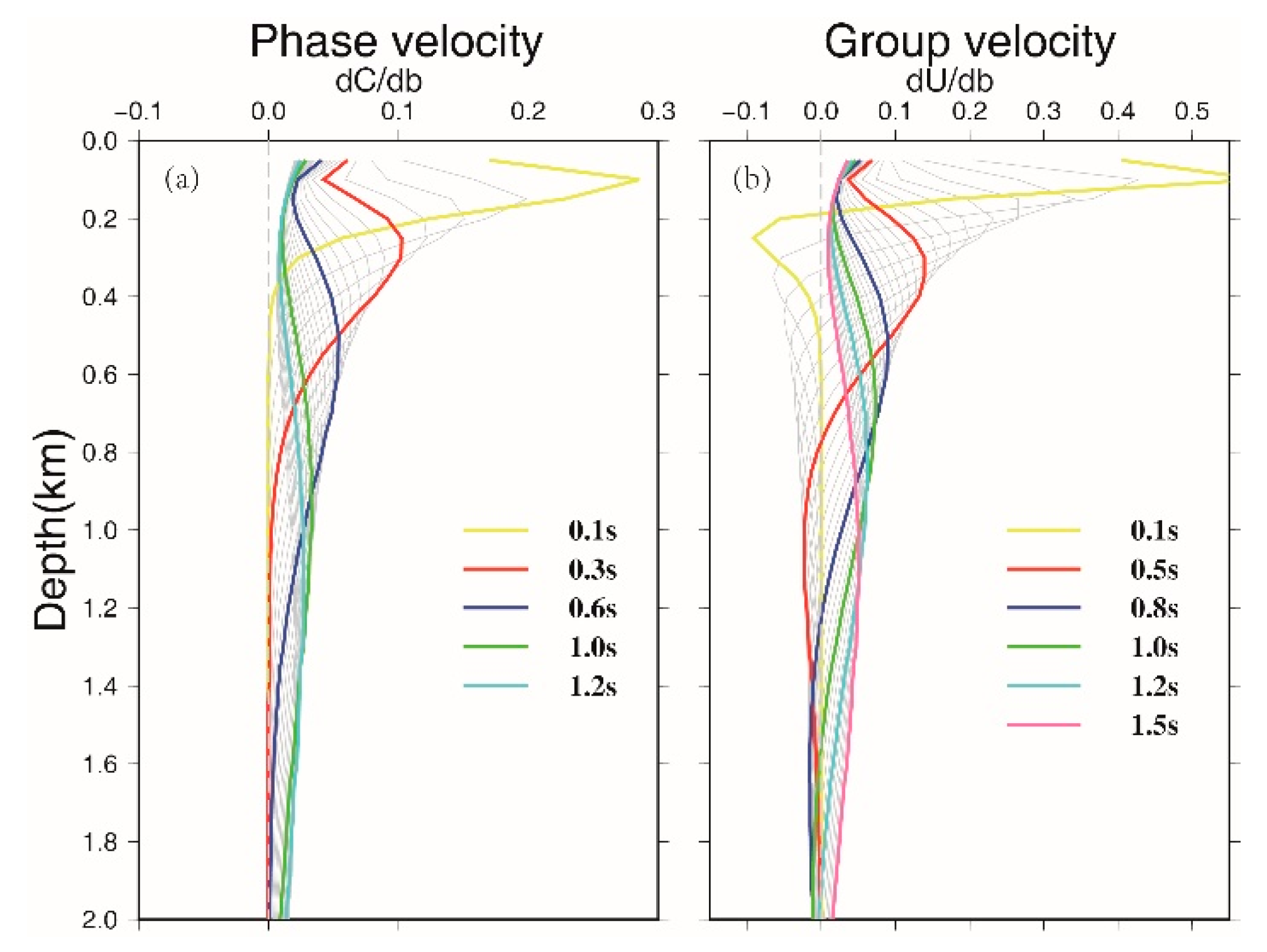
Empirically proven relationships suggest that the fundamental mode Rayleigh-wave phase velocity is mostly sensitive to the shear-wave velocity at depths about one-third of its corresponding wavelength [24,28] and phase velocity is 0.92 of shear-wave velocity at a uniform half-space Poisson solid [28]. We constructed an initial 1D shear-wave velocity model and adjusted it according to CRUST 1.0 [29] (Figure S3). Then the srfker96 program in Computer Programs in Seismology was used to solve the depth sensitivity kernels (Figure 5) depending on the input of the 1D shear-wave velocity model at a given frequency [30]. The sensitive kernel functions, corresponding to the selected periods plotted in Figure 5, show that phase and group velocities are complementary in depth. In addition, when phase and group velocities are inverted simultaneously, uncertainties are significantly reduced at depths [31], suggesting that joint inversion of group velocity and phase velocity may help to increase the robustness of the inverted velocity model.
We subsequently applied a direct inversion imaging technique [24] to invert both surface wave dispersions for the 3D shallow crustal shear-wave velocity structures beneath the mine. The method is based on 2D ray tracing instead of surface-wave propagating along the great-circle path, which is more suitable for complex situations in the shallow crust where large velocity variations usually cause strong non-linear effects. Next, a fast-marching method [32] was used to calculate Rayleigh-wave travel-time. Traditional inversion approaches do not usually update ray paths and sensitivity kernels for the updated 3D models, which may bias computation in wave propagation and thus invert velocity models in complex mediums [24]. In the computation of direct inversion imaging, the 3D wave speed model at each inversion step was used to obtain the 2D phase velocity maps and to construct new depth sensitivity kernels. Essentially these laterally varying depth kernels were updated with each iteration of inversion so that more accurate kernels were considered. Inversion parameters (e.g., weight factor between data misfit and model smoothing [24]) are tested at the beginning to obtain an optimal residual distribution [24,33]. Finally, we used all the parameters obtained from previous calculations to inverse for a 3D shear-wave velocity structure of Karatungk Mine.
3. Results
We jointly inverted group and phase velocity dispersion data to obtain the shallow crustal shear velocity structures. The study area was parameterized into a 36 by 36 grid points on the horizontal plane and 20 grid points along the depth direction. The grid size of the latitude and longitude in the horizontal plane are 0.0102° and 0.0147°, and in depth the grid interval varies from 50 m to 300 m within the depth of 1.3 km.
3.1. Resolution Tests
In order to test the robustness of the inversion results, we conducted a series of resolution tests (Figure S4). These tests illustrate that our dataset may reach a lateral resolution of ~1.0 km at shallow depth (<0.2 km) and 1.3 km at deep depth, respectively. In Figure 6 we show the residual distribution of initial inversion and last inversion. After the iterative, non-linear inversion, the distribution of travel time residuals is more Gaussian-like, and the average and standard deviation of the residuals dropped significantly from −0.022 s and 0.197 s in the initial model to 0.001 s and 0.076 s in the final model, respectively (Figure 6).
3.2. Error Analysis
In order to improve the accuracy and stability of the inversion results for all dispersion curves, here we adopted a bootstrap resampling method with repeated sampling of dispersion curves [34], then multiple sets of dispersion curves can be used for inversion. We performed the bootstrap procedure in which 50 sets of resampled dispersion curves were generated and then inverted for 50 velocity models. We used the resulting mean and standard deviation of the velocity models as the final model and the approximated model error, respectively (Figure 7). There are only few ANT studies that deal with model errors at this step, e.g., [24,35]. Here the bootstrap procedure has the advantage to deal with real data errors without any assumptions, for example the distribution, the amplitude, and different sources of error that cannot be explained by an inversion problem. Figure 7 shows the velocity structure of the imaging results, in which the mean and standard deviation of the velocity structure were obtained by the bootstrap resampled datasets. We found that the bootstrapped average velocity structure is very close to the velocity structure inverted from the original data set (Figure S5). The model errors approximated by the standard deviation allow us to evaluate robust model regions for interpretation, for example, in most areas the approximated model errors are <~1.0–1.2% level (Figure 7 and Figure S6). These measures provide confidence that the results are robust. The bootstrap procedure restricts the description of error to the dataset used in this study; thus, the error estimate described here is not transferrable to other regions or datasets. Nonetheless, the approach is transferrable to other regions and datasets in order to provide a useful measure from which robustness is represented to guide predictive endeavours. We stress that the model error obtained this way is not in the absolute sense, but this “approximated” approach helps us determine reliable model features.
3.3. Shear-Wave Velocities
Figure 7, Figure 8 and Figure 9 present the new features of our absolute shear-wave velocity model beneath Karatungk Mine. In the shallow section within 0.5 km depth, the shear-wave velocity maps show that prominent low velocities (<2.55 km/s) spatially correspond to the major ore-hosting intrusions Y1 and northwest of Y2 (Figure 8), while high velocities (2.7–3.3 km/s) are present in Y3 and southeast of Y2, which extends vertically to ~0.6 km depth (Figure 8). Another major feature is a low-velocity zone (LVZ) of 1.5–2 km width beneath Y2 and Y3 at a depth of 0.7–1.3 km (Figure 8). In this depth range, we also find high-velocity zones (HVZs) in the northernmost and the southernmost sections of the study area at a depth of 0.7–1.3 km.
Depth cross-sections of the velocity structure are shown in Figure 9. The high-velocity anomalies (3.25–3.6 km/s) mentioned above are observed on sections A–A′, B–B′, and C–C′. The high-velocity anomalies are thinner in the middle of the section and thicker on both sides (Figure 9). In sections A–A′ to C–C′, the LVZs, locating in the middle of the mine, gradually expand horizontally from northeast to southwest and vertically expand from 1.0–1.3 km to 0.7–1.3 km. Additionally, a thin high-velocity anomaly, also located in the middle of the mine, is proximal to the LVZ beneath Y2 and Y3 at section B–B′ (Figure 9). Profiles D–D′, E–E′, and F–F′ in Figure 9 intersect Y1, Y2, and Y3, respectively. The HVZ beneath Y1 in D–D′ is much thicker than the zone beneath Y2 in E–E′, and the HVZ beneath Y3 in F–F′ is estimated to be the thinnest among those proximal to Y3, Y2, and Y1 (Figure 9).
4. Discussion
In this paper, we applied the ANT to the dense passive-source array data to image a mining area in northeastern Xinjiang, China. We found clear velocity heterogeneities in the study area that spatially coincide with the major ore-hosting intrusions. We attempt to interpret their geological meaning here (Figure 8 and Figure 9). In the following section, we discuss the structure at depths 0–0.7 km and 0.7–1.3 km, respectively. The velocity structure is considered to be in two sections as the major ore-hosting intrusions are suggested by borehole observations to be distributed at 0–0.7 km depth [5,10] where the model errors are also considerably small (Figure S6). The deeper part (0.7–1.3 km), were considered as the source regions of these ore-hosting intrusions [36].
4.1. Seismic Structure within 0.7 km and Y1, Y2, Y3
The major pattern of the seismic structure at Karatungk Mine within 0.7 km is that three main ore-hosting intrusions present different velocity features (Figure 8 and Figure 9). Y1 and northwest of Y2 present relatively LVZs (<2.55 km/s) at the depth of 0–0.5 km. Y3 and southeast of Y2 present HVZs (2.7–3.3 km/s) at a depth of 0–0.6 km. Horizontal checkerboard tests show that horizontal resolution of our measurements may reach ~1.0 km, indicating that Y1 and Y2 are distinguishable from each other. We performed vertical synthetic model tests by setting six velocity anomalies with different thickness in depth (Figure S7), each of which has the same distribution of synthetic anomalies, and its depth range is equal to the thickness of the anomalies. Vertical recoveries of tests (Figure S7) suggest that a depth resolution of 0.1 km in the region shallower than 0.4 km may be reasonably recovered, i.e., the tests in Figure S7 show that even vertical smearing of ~0.1km may occur, the centers of the anomalies are well recovered at correct depths. This confirms the reliability of the LVZs distributed at Y1 and northwest of Y2 at depths of 0–0.5 km, and HVZs at southeast of Y2 and Y3 at depths of 0–0.6 km. We focus on the velocity features of Y1–Y3 here since imaging has limited resolutions near Y4–Y9 (Figure 1) and most published works of Karatungk Mine relate to Y1–Y3. Figure S6 further illustrates that these three features are in very small model error regions (<1.0%).
Factors contributing to the velocity features nature of the featureY1–Y3 mentioned above include lithology, water content, and degree of mineralization for the ore-hosting intrusions. The observed lithologies of Y1 are biotite gabbro, amphibolite, hyperite, and diabase gabbro; Y2 are bojite, norite, and gabbro; and Y3 are gabbro-diorite, bojite, and amphibolite [5]. Overall there is little difference in lithology compositions that would differentiate these bodies in velocity structure According to lithology and composition, the ore-hosting intrusions comprise multiple hydrous minerals, which indicate early magma intrusion was relatively hydrous [37]. Considering that the hydrous minerals evolve under the same tectonic conditions, we reasonably deduce that water is not a predominant discriminating factor. According to previous geological studies and borehole data, the mineralization of three major ore-hosting intrusions indicates that Y1 and northwestern part of Y2 are strongly mineralized, while the southeast of Y2 has a weaker degree of mineralization, and Y3 presents weak mineralization [5]. Previous studies suggest a relationship between mineralization and velocity. For example, [10] suggest that compressional velocity decreases with an increase of mineralization of gabbroic rocks. Additionally, based on the results of borehole petrophysic experiments at Voisey’s Bay Cu-Ni sulfide mine from [38], the highly-mineralized sulfide shows higher density but lower seismic wave velocity compared with the host rocks. Other studies, while not specifically describing Cu-Ni mineralization, do investigate similar styles of mineralization and report a similar relationship between sulfidation and velocity [39,40]. To summarize, the rock composition and water content of three ore-hosting intrusions show few differences. As levels of mineralization are consistent with changes in velocity features in our study, we speculate the spatial variations of the shear-wave velocity may be mainly related to the distribution of mineralization.
4.2. Seismic Structure at the Depth of 0.7–1.3 km
The major feature at the depths of 0.7–1.3 km is an LVZ of approximate width 1.5–2 km beneath Y2 and Y3 (Figure 8). Resolution tests show that our dataset can retrieve structures of similar size at the depth (Figure S3), although these structures are located in relatively large model error regions (up to 2%; Figure S6). We propose three candidates for the origin. First, we speculate that the LVZ beneath Y2 and Y3 may be the possible channel for initial magma transport. A continuous supply for magma suggests that the older host rocks of this area would cool earlier than the intrusions, and possibly exhibit higher velocities. The second speculation is inspired by the drilling data obtained from beneath Y3 and Y5, which show that siliceous rocks and a fragmentation zone exist at depths >1.1 km [10]. From results at 0–0.6 km depth, the tuff and weakly mineralized intrusive rocks would be indistinguishable in terms of shear-wave velocity. With the support of borehole data, we further realize that LVZ beneath Y2 and Y3 at the depth of 0.7–1.3 km may also correspond to the strata observed in the mine, of which are predominantly carbonaceous tuff, argillaceous tuff, and coarse-grained tuff. Since we do not have enough constraints for fault distribution in the mine, we are unable to correlate this velocity feature to a possible fragmentation zone beneath Y2 and Y3 without further drilling data. The last speculation is that the relative LVZ near the intrusive rocks might indicate a possible mineralized area according to the arguments presented in Section 4.1 linking mineralization can and lower velocities [10,38].
We find HVZs in the northernmost and the southernmost sections of the study area at a depth of 0.7–1.3 km. Prior investigations of ore-hosting lithology in the mine indicate that main intrusive rocks are gabbro and hyperite of the middle-late Hercynian age. Laboratory measurements suggest that less mineralized gabbro has a higher velocity [9]. Thus we suggest that HVZs may be connected with un-mineralized intrusive rocks (e.g., gabbro, peridotite and gabbro-diabase) resulting from early magma intrusion.
4.3. Passive Observations Based on a Dense Array
This study demonstrates a new application of ANT to a dense array in a mine, trying to provide a general connection between seismic velocity, the seismic images and Cu-Ni sulfide orebodies. This relationship contributes to a better understanding of the shallow mineralization processes beneath Karatungk Mine. The major limitation of this study is the resolution of tomographic imaging. Resolution, however, can be improved by increasing the number of seismometers and reducing the station spacing.
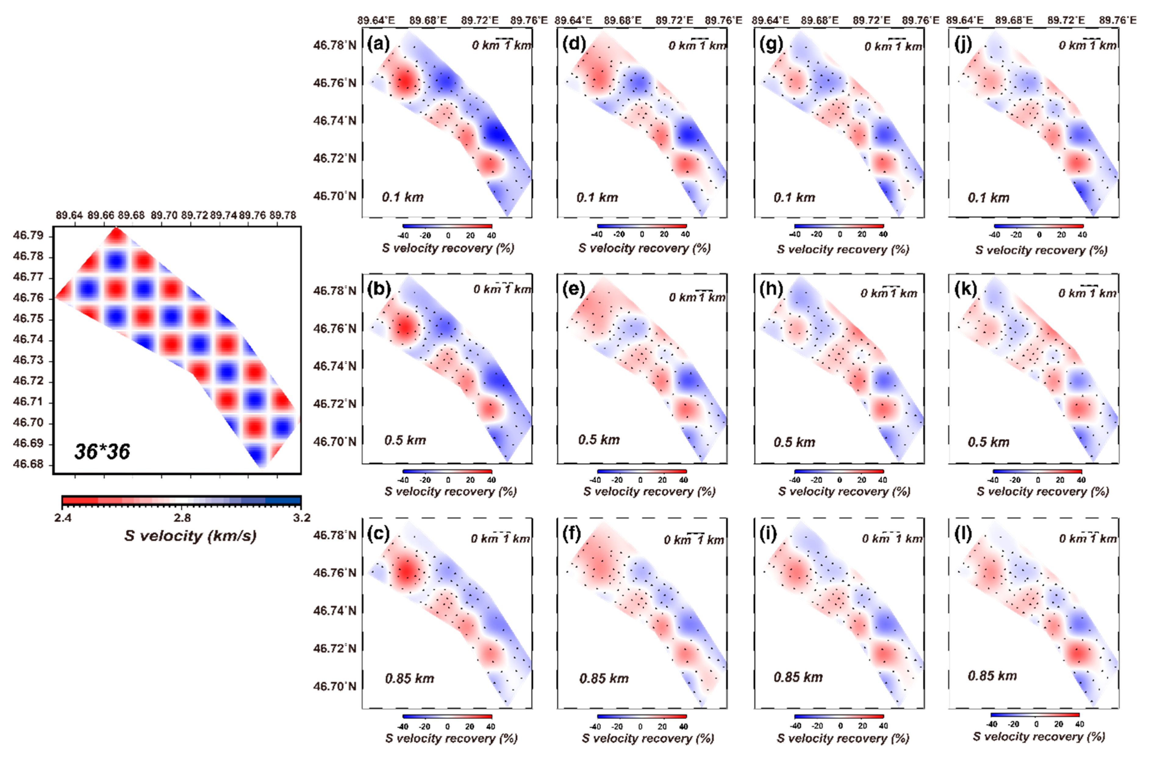
Firstly, to demonstrate that increasing the number of stations can effectively improve the resolution of inversion results in the case of a specific study area, we used a jackknife-style resampling approach [41] to artificially select 50%, 70%, and 90% of stations from the original 100 stations. Then, we used dispersion curves corresponding to the selected stations for horizontal resolution tests. Theoretical model and inversion parameters used in the test are the same as those in Section 3.1. Figure 10 shows the comparison of resolution tests corresponding to different numbers of stations (50, 70, and 90) and various depths (0.1 km, 0.5 km, and 0.85 km) to the original data (100 stations). It is clear that for a grid size of 0.1° × 0.14°, using only 50 stations results in difficulties in recovering the input model for most regions. By increasing the number of stations, recovery of the input model at depths of 0.1, 0.5, and 0.85 km are improved systematically. When the number of samples reaches 90, the resolution tests show similar recovery of that from the original dataset (100 stations). This shows that under these conditions, increasing the number of ray paths, by deploying more stations, can improve the resolution to a certain degree.
4.4. Potential of Seismic Observations in Deep Prospecting Work
Another major difficulty in this study, and indeed in many mining locations, is the complex structure of the ore bodies. The uneven mineralization distribution of ore-hosting intrusions and the different degrees of mineralization can result in various velocity characteristics. Thus, determining the distribution of Cu-Ni sulfide orebodies is not easily obtained by seismic imaging alone. Indeed, some geological control from direct observation or sampling will always be required to support interpretation of mineralized zones from geophysics. Furthermore, in Karatungk Mine, magnetic and gravity anomalies have a consistent surface correlation with the ore bodies (Y1 to Y9) inferred from earlier multi-disciplinary studies [5] (Figure 11a,b). These geophysical datasets, however, do not distinguish the orebodies’ depth distribution, and mineralization extent of orebodies so far depends on more expensive surface and in-tunnel drilling data (Figure 11c). With limited spatial resolution, the seismic model here seems to favor a positive correlation between the two highly mineralized regions beneath Y1 and Y2 (red open blocks in Figure 11c) and the shallowing trending slow velocity (Figure 11d), and between the low mineralized regions beneath Y2 and Y3 (blue dashed open blocks) and the high velocities towards the bottom of the orebodies (Figure 11c,d). We conclude that complementary to expensive direct observation and sampling, less expensive reconnaissance surveys as described here can mitigate the risk of drilling activities. In the future, we may better solve this issue with the help of multiple geophysical observations; however, this technique demonstrates a feasible reconnaissance method that can provide useful initial images to better guide more expensive and invasive mineral exploration methods.
5. Conclusions
We have demonstrated a technique to recover a shallow crustal shear-wave velocity structure beneath Karatungk Mine, Junggar Basin, using ANT based on KMA. We observe that low-velocity heterogeneities are mainly distributed near the Y1 ore-hosting intrusion and northwest of Y2 within ~0.5 km depth. In addition, high-velocity heterogeneities are mainly located at the southeast of Y2 and Y3 within ~0.7 km depth. We proposed that the spatial variations of the shear-wave velocity may mainly be related to the mineralization of three ore-hosting intrusions, which is supported by other studies and qualitative reasoning. We also observe that low velocities beneath Y2 and Y3 at depths of 0.7–1.3 km. We interpret that these low-velocity zones may indicate the presence of magmatic conduits, mine strata or mineralized regions. High-velocity anomalies displayed in the northernmost and southernmost sections of the mine at depths of 0.7–1.3 km are interpreted to relate to the intrusions of gabbro, peridotite, and gabbro-diabase resulting from the early magmatism.
Our study demonstrates an applicable technique for using passive seismic imaging at the mine-scale for the first time, which can then help us to better understand the shallow structure of Karatungk Mine, and mining environments in general. ANT method using a dense array is shown to be a potentially efficient way to reveal detailed structure in mine areas. In this example, ore-hosting intrusions within 0.7 km in depth have been well-constrained and supported by borehole data observations. However, variable spatial distribution of mineralization and complex ore-body geometry can cause difficulties in determining the exact location of Cu-Ni sulfide orebodies. In addition, the spatial resolution of the results is still too low to solve the geometry of all Cu-Ni sulfide orebodies. However, we successfully demonstrate that a denser ANT array will obtain more detailed structure in the area.
Supplementary Materials
The following are available online at https://www.mdpi.com/2075-163X/10/7/601/s1, Section S1: Beamforming of Cross-Correlation Functions; Section S2: Resolution, Robustness Tests and Model Error Estimates; Figure S1: Distribution of ambient noise sources along different azimuths and slowness; Figure S2: Results of fundamental mode Rayleigh wave dispersion measurement; Figure S3: Starting 1D velocity model (red), which is also used for depth kernel computation; Figure S4: Horizontal resolution tests; Figure S5: Model comparison between models without (left) and with bootstrap approach (right); Figure S6: Same as the cross-sections in Figure 9 but for approximated model errors using the bootstrap procedure; Figure S7: Vertical synthetic model tests.
Author Contributions
Conceptualization, J.W., C.H., J.W., L.Z., and W.X.; methodology, P.D., J.W., and H.Y.; software, P.D.; data curation, P.D., J.W., Y.L., J.W., and C.H.; writing—original draft preparation, P.D. and J.W.; writing—review and editing, J.W., Y.L., M.D.L., H.Y., and L.Z.; supervision, J.W.; and project administration, J.W., L.Z., and W.X. All authors have read and agreed to the published version of the manuscript.
Funding
This research was funded by the National Key R&D Programs of China (Grant No.2017YFC0601206 and Grant No.2017YFC1500302), National Natural Science Foundation of China (Grant No.41574055), State Key Laboratory of Lithospheric Evolution, Institute of Geology and Geophysics, Chinese Academy of Sciences (Grant No.11731210).
Acknowledgments
Zhengfu Guo, Kezhang Qin, Yibo Wang and Dongmei Tang from the Institute of Geology and Geophysics and the Chinese Academy of Sciences, and Nishida Kiwamu from the Earthquake Research Institute, Tokyo University, provided great supports for this study. Thanks to Zhihai Li, Xiaomei Liu, Jujing Li, Shaojiang Wu, and Xianzhen Chen for their help in the field work. Group members of Crustal and Mantle Structure from State Key Laboratory of Lithospheric Evolution helped a lot on this study. Support from the Computer Simulation Lab, Institute of Geology and Geophysics, and the Chinese Academy of Sciences is appreciated. The figures are produced by GMT [42]. Mark Lindsay acknowledges the support from ARC DECRA Scheme project number DE190100431. HY acknowledges partial support from NSFC programs 91955210, 41625016 and CAS program GJHZ1776. This is Contribution 1514 from the ARC Centre of Excellence for Core to Crust Fluid Systems (http://www.ccfs.mq.edu.au).
Conflicts of Interest
The authors declare no conflict of interest.
References
- Han, C.; Xiao, W.; Zhao, G.; Qu, W.; Mao, Q.; Du, A. Re-Os isotopic analysis of the Kalatongke Cu-Ni Sulfide Deposit, Northern Xinjiang, NW China, and its geological implication. Acta Petrol. Sin. 2006, 22, 163–170, (In Chinese with English abstract). [Google Scholar]
- Wang, J. The Minerogenesis and Metallogenic Potential of Kalatongke Nickel -Copper Sulfide Deposit, Xinjiang, China. Ph.D. Thesis, Chang’an University, Xi’an, China, 2010. (In Chinese with English abstract). [Google Scholar]
- Wan, B.; Xiao, W.; Windley, B.F.; Yuan, C. Permian hornblende gabbros in the Chinese Altai from a subduction-related hydrous parent magma, not from the Tarim mantle plume. Lithosphere 2013, 5, 290–299. [Google Scholar] [CrossRef] [Green Version]
- Gong, Y.; Wang, Y.; Wang, B. Exploration on resource prediction in karatungk Cu-Ni metallogenic belt. Xinjiang Nonferrous Met. 2005, A2, 32–35, (In Chinese with English abstract). [Google Scholar]
- Qin, K.; Tian, Y.; Yao, Z.; Wang, Y.; Mao, Y.; Wang, B.; Xue, S.; Tang, D.; Kang, Z. Metallogenetic conditions, magma conduit and exploration potential of the kalatongk Cu-Ni orefield in Northern Xinjiang. Geol. China 2014, 41, 912–935, (In Chinese with English abstract). [Google Scholar]
- Han, C.; Wenjiao, X.; Guochun, Z.; Wenjun, Q.; Andao, D. Re–Os dating of the Kalatongke Cu–Ni deposit, Altay Shan, NW China, and resulting geodynamic implications. Ore Geol. Rev. 2007, 32, 452–468. [Google Scholar] [CrossRef]
- Ferguson, I.J.; Young, J.B.; Cook, B.J.; Krakowka, A.B.C.; Tycholiz, C. Near-surface geophysical surveys at the Duport gold deposit, Ontario, Canada: Relating airborne responses to small-scale geologic features. Interpretation 2016, 4, SH39–SH60. [Google Scholar] [CrossRef]
- Malehmir, A.; Juhlin, C.; Wijns, C.; Urosevic, M.; Valasti, P.; Koivisto, E. 3D reflection seismic imaging for open-pit mine planning and deep exploration in the Kevitsa Ni-Cu-PGE deposit, northern Finland. Geophysics 2012, 77, 95–108. [Google Scholar] [CrossRef] [Green Version]
- Tong, T.; Hu, X.; Liu, J. Study of Metallogenic Forecast and Geophysical Characteristics in Copper-nickel Mine of Kalatongke. West-China Explor. Eng. 2004, 9, 105–106, (In Chinese with English abstract). [Google Scholar]
- Zhou, J.; Xu, M.; Liu, J.; Gao, J.; Wang, X.; Zhang, B. Application of seismic reflection imaging in the Karatungk Cu-Ni deposit of Xinjiang. Geol. Explor. 2016, 52, 0910–0917, (In Chinese with English abstract). [Google Scholar]
- Lin, F.-C.; Ritzwoller, M.H.; Snieder, R. Eikonal tomography: Surface wave tomography by phase front tracking across a regional broad-band seismic array. Geophys. J. Int. 2009, 177, 1091–1110. [Google Scholar] [CrossRef] [Green Version]
- Wang, Y.; Allam, A.; Lin, F.-C. Imaging the Fault Damage Zone of the San Jacinto Fault Near Anza With Ambient Noise Tomography Using a Dense Nodal Array. Geophys. Res. Lett. 2019, 46, 12938–12948. [Google Scholar] [CrossRef]
- Lin, F.-C.; Li, D.; Clayton, R.W.; Hollis, D. High-resolution 3D shallow crustal structure in Long Beach, California: Application of ambient noise tomography on a dense seismic array. Geophysics 2013, 78, Q45–Q56. [Google Scholar] [CrossRef] [Green Version]
- Sabra, K.G.; Gerstoft, P.; Roux, P.; Kuperman, W.A.; Fehler, M.C. Extracting time-domain Green’s function estimates from ambient seismic noise. Geophys. Res. Lett. 2005, 32, L03310. [Google Scholar] [CrossRef]
- Shapiro, N.M.; Campillo, M.; Stehly, L.; Ritzwoller, M.H. High-Resolution Surface-Wave Tomography from Ambient Seismic Noise. Science 2005, 307, 1615–1618. [Google Scholar] [CrossRef] [PubMed] [Green Version]
- Yao, H.; Hilst, R.D.V.D.; Hoop, M.V.D. Surface-wave array tomography in SE Tibet from ambient seismic noise and two-station analysis—I. Phase velocity maps. Geophys. J. Int. 2006, 166, 732–744. [Google Scholar] [CrossRef] [Green Version]
- Lin, F.-C.; Moschetti, M.P.; Ritzwoller, M.H. Surface wave tomography of the western United States from ambient seismic noise: Rayleigh and Love wave phase velocity maps. Geophys. J. Int. 2008, 173, 281–298. [Google Scholar] [CrossRef] [Green Version]
- Saygin, E.; Kennett, B.L.N. Crustal structure of Australia from ambient seismic noise tomography. J. Geophys. Res. 2012, 117. [Google Scholar] [CrossRef] [Green Version]
- Yang, Y.; Ritzwoller, M.H.; Levshin, A.L.; Shapiro, N.M. Ambient noise Rayleigh wave tomography across Europe. Geophys. J. Int. 2007, 168, 259–274. [Google Scholar] [CrossRef] [Green Version]
- Keifer, I.; Dueker, K.; Chen, P. Ambient Rayleigh wave field imaging of the critical zone in a weathered granite terrane. Earth Planet. Sci. Lett. 2019, 510, 198–208. [Google Scholar] [CrossRef]
- Roux, P.; Moreau, L.; Lecointre, A.; Hillers, G.; Campillo, M.; Ben-Zion, Y.; Zigone, D.; Vernon, F. A methodological approach towards high-resolution surface wave imaging of the San Jacinto Fault Zone using ambient-noise recordings at a spatially dense array. Geophys. J. Int. 2016, 206, 980–992. [Google Scholar] [CrossRef] [Green Version]
- Yao, H.; Xu, G.; Zhu, L.; Xiao, X. Mantle structure from inter-station Rayleigh wave dispersion and its tectonic implication in Western China and neighboring regions. Phys. Earth. Planet. In. 2005, 148, 39–54. [Google Scholar] [CrossRef]
- Yao, H.; Gouédard, P.; Collins, J.; McGuire, J.; van der Hilst, R.D. Structure of young East Pacific Rise lithosphere from ambient noise correlation analysis of fundamental- and higher-mode Scholte-Rayleigh waves. Comptes Rendus Geosci. 2011, 343, 571–583. [Google Scholar] [CrossRef]
- Fang, H.; Yao, H.; Zhang, H.; Huang, Y.-C.; van der Hilst, R.D. Direct inversion of surface wave dispersion for three-dimensional shallow crustal structure based on ray tracing: Methodology and application. Geophys. J. Int. 2015, 201, 1251–1263. [Google Scholar] [CrossRef] [Green Version]
- Bensen, G.D.; Ritzwoller, M.H.; Barmin, M.P.; Levshin, A.L.; Lin, F.; Moschetti, M.P.; Shapiro, N.M.; Yang, Y. Processing seismic ambient noise data to obtain reliable broad-band surface wave dispersion measurements. Geophys. J. Int. 2007, 169, 1239–1260. [Google Scholar] [CrossRef] [Green Version]
- Yao, H.; Beghein, C.; van der Hilst, R.D. Surface wave array tomography in SE Tibet from ambient seismic noise and two-station analysis–II. Crustal and upper-mantle structure. Geophys. J. Int. 2008, 173, 205–219. [Google Scholar] [CrossRef] [Green Version]
- Luo, Y.; Yang, Y.; Xu, Y.; Xu, H.; Zhao, K.; Wang, K. On the limitations of interstation distances in ambient noise tomography. Geophys. J. Int. 2015, 201, 652–661. [Google Scholar] [CrossRef] [Green Version]
- Shearer, P.M. Introduction to Seismology, 2nd ed.; Cambridge University Press: New York, NY, USA, 2009. [Google Scholar]
- Laske, G.; Masters, G.; Ma, Z.; Pasyanos, M. Update on CRUST1.0—A 1-degree global model of Earth’s crust. Geophys. Res. Abstr. 2013, 15, 2658. [Google Scholar]
- Herrmann, R.B. An Overview of Synthetic Seismogram Computation, Computer Programs in Seismology; Saint Louis University: Baguio, Benguet, 2002. [Google Scholar]
- Shapiro, N.M.; Ritzwoller, M.H. Monte-Carlo inversion for a global shear-velocity model of the crust and upper mantle. Geophys. J. Int. 2002, 151, 88–105. [Google Scholar] [CrossRef] [Green Version]
- Rawlinson, N.; Sambridge, M. Wave front evolution in strongly heterogeneous layered media using the fast marching method. Geophys. J. Int. 2004, 156, 631–647. [Google Scholar] [CrossRef] [Green Version]
- Liu, Y.; Zhang, H.; Fang, H.; Yao, H.; Gao, J. Ambient noise tomography of three-dimensional near-surface shear-wave velocity structure around the hydraulic fracturing site using surface microseismic monitoring array. J. Appl. Geophys. 2018, 159, 209–217. [Google Scholar] [CrossRef]
- Efron, B.; Tibshirani, R. Bootstrap methods for standard errors, confidence intervals, and other measures of statistical accuracy. Stat. Sci. 1986, 1, 54–77. [Google Scholar] [CrossRef]
- Li, T.; Zhao, L.; Wan, B.; Li, Z.X.; Bodin, T.; Wang, K.; Yuan, H. New crustal Vs model along an array in south-east China: Seismic characters and paleo-Tethys continental amalgamation. Geochem. Geophys. Geosyst. 2020, 21, e2020GC009024. [Google Scholar] [CrossRef]
- Zhou, J. The application of seismic method in deep prospecting–take the case of the Cu-Ni deposit in Karatungk of Xinjiang Province. Ph.D. Thesis, China University of Geosciences, Wuhan, China, 2017. (In Chinese with English abstract). [Google Scholar]
- Chai, F. Comparison on Petrologic Geochemistry of Three Mafic-ultramafic instrusions Associated with Ni-Cu Sulfide Deposits in Northern Xinjiang. Ph.D. Thesis, China University of Geosciences, Wuhan, China, 2006. (In Chinese with English abstract). [Google Scholar]
- Duff, D.; Hurich, C.; Deemer, S. Seismic properties of the Voisey’s Bay massive sulfide deposit: Insights into approaches to seismic imaging. Geophysics 2012, 77, 59–68. [Google Scholar] [CrossRef]
- Shetselaar, E.; Bellefleur, G.; Craven, J.; Roots, E.; Cheraghi, S.; Shamsipour, P.; Caté, A.; Mercier-Langevin, P.; El Goumi, N.; Enkin, R.; et al. Geologically Driven 3D Modelling of Physical Rock Properties in Support of Interpreting the Seismic Response of the Lalor Volcanogenic Massive Sulphide Deposit, Snow Lake, Manitoba, Canada; Geological Society: London, UK, 2017; Volume 453. [Google Scholar]
- Dentith, M.; Enkin, R.J.; Morris, W.; Adams, C.; Bourne, B. Petrophysics and mineral exploration: A workflow for data analysis and a new interpretation framework. Geophys. Prospect. 2020, 68, 178–199. [Google Scholar]
- Efron, B. Bootstrap Methods: Another Look at the Jackknife. Ann. Stat. 1979, 7, 1–26. [Google Scholar] [CrossRef]
- Wessel, P.; Smith, W.H.F.; Scharroo, R.; Luis, J.; Wobbe, F. Generic Mapping Tools: Improved Version Released. Eos Trans. Am. Geophys. Union 2013, 94, 409–410. [Google Scholar] [CrossRef] [Green Version]
Figure 1.
Karatungk Mine, local geological setting, and seismic array. (a) Topographic map and the Karatungk Mine array—KMA. The map shows the location of KMA (black triangles). Blue solid lines show the profiles across the mine on which velocity model is presented. Red areas represent the ore-hosting intrusions. White letters are the name of intrusions. (b) The regional map of Karatungk Mine: black lines are faults and red triangles show the permanent stations in Xinjiang Province, yellow circles show the seismicity from China Earthquake Network Center. The inset shows the geographic location of this map. The white rectangle shows the geographic location of (a). (c) Detailed distribution of ore-hosting intrusions (Y1–Y11) in Karatungk Mine, modified from [5]. Labels of horizontal and vertical axis are the location of the mine given in Geodetic coordinate system. Right panel shows detailed structural attributes.

Figure 2.
An example of cross-correlation functions (CCFs) used for dispersion measurements in the periods of 0.1–2 s. The CCFs of the total 58 days between 10 stations (named as XJ100~XJ109) and all the other stations of KMA. CCFs shown here are not symmetrized waveforms.
Figure 2.
An example of cross-correlation functions (CCFs) used for dispersion measurements in the periods of 0.1–2 s. The CCFs of the total 58 days between 10 stations (named as XJ100~XJ109) and all the other stations of KMA. CCFs shown here are not symmetrized waveforms.

Figure 3.
Rayleigh wave group (a) and phase (b) velocity dispersion curves analysis. Different color shows envelope amplitude at different period and velocity; blue presents lower amplitude and yellow brown show higher amplitude. (a) Rayleigh wave group velocity dispersion curves analysis. The horizontal axis is period (s) and the vertical axis is group velocity (km/s). Blue circles are the dispersion points satisfying the threshold of which only red-filled points are saved for inversion. The dark line is the dispersion curve which is predicted by the code. (b) Rayleigh wave phase velocity dispersion curves analysis. Horizontal axis is period (s) and vertical axis is group velocity (km/s). Pink line (bottom) shows the group velocity dispersion curves extracted in the previous step, which is used as a reference to guide picking of the corresponding phase velocity dispersion curve.

Figure 4.
Ray path density maps of Rayleigh wave dispersion curves between all stations at various periods, and 0.1 s, 0.5 s, 0.7 s, 1.1 s are presented, respectively. (a–d) Ray path density maps of phase velocity; (e–h) Ray path density maps of group velocity.
Figure 4.
Ray path density maps of Rayleigh wave dispersion curves between all stations at various periods, and 0.1 s, 0.5 s, 0.7 s, 1.1 s are presented, respectively. (a–d) Ray path density maps of phase velocity; (e–h) Ray path density maps of group velocity.

Figure 5.
Rayleigh wave depth sensitivity kernels at different periods. (a) The sensitivity kernels of the phase velocity. (b) The sensitivity kernels of the group velocity. Gray curves show the kernels with 0.1 s increments in between the labeled periods.
Figure 5.
Rayleigh wave depth sensitivity kernels at different periods. (a) The sensitivity kernels of the phase velocity. (b) The sensitivity kernels of the group velocity. Gray curves show the kernels with 0.1 s increments in between the labeled periods.

Figure 6.
Distributions of surface wave travel-time residuals. Residuals before inversion are gray columns with the average μ = −0.022 s and the standard deviation σ = 0.197 s. Residuals after inversion are red columns with μ = 0.001 s and σ = 0.076 s.
Figure 6.
Distributions of surface wave travel-time residuals. Residuals before inversion are gray columns with the average μ = −0.022 s and the standard deviation σ = 0.197 s. Residuals after inversion are red columns with μ = 0.001 s and σ = 0.076 s.

Figure 7.
The Vs model and approximated model errors from the bootstrap inversion. The final Vs model is averaged from the 50 models inverted using bootstrapped datasets, and is shown at 0.1, 0.5, 0.7 and 1.0 km, respectively in the top panels. The model errors approximated from the standard deviation are plotted in the lower panels. The errors are in general in the range of ~0.2% to 2.7%. (Note outside the array there is no ray coverage. The <0.2% errors reflect smoothing and regularization in the effective regions and therefore may not be representative of robust regions). White areas with black solid lines represent the surface location of ore hosting intrusions Y1–Y9.

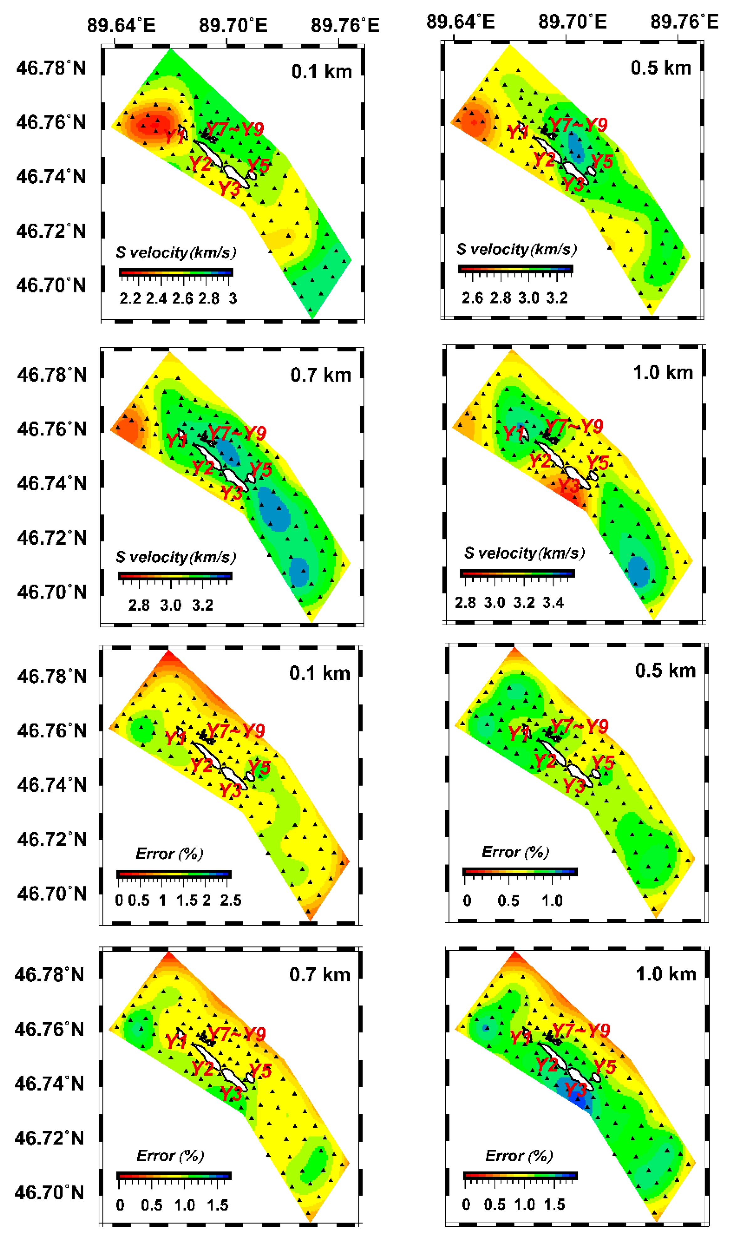
Figure 8.
Left panel shows 3D shear wave velocity slices at the depth of 0.1, 0.2, 0.3, 0.4, 0.5, 0.6, 0.7, 0.85, 1.0, 1.15 and 1.30 km, respectively. Black lines at the left top panel of topographic pattern and black dotted lines at 0.1~0.7 km in the lower panel all show ore hosting intrusions. Red solid rectangles represent LVZs at Y1 and northwest of Y2. Blue dotted rectangles indicate HVZs southeast of Y2 and Y3. Right panel represents horizontal slices of shear wave velocity in the mine at the depth of 0.2, 0.3, 0.4, 0.6, 0.85 and 1.3 km (a–f). Areas circled by blue lines on the upper panel and yellow lines on the bottom panel are the ore-hosting intrusions Y1~Y9 in Karatungk mine.

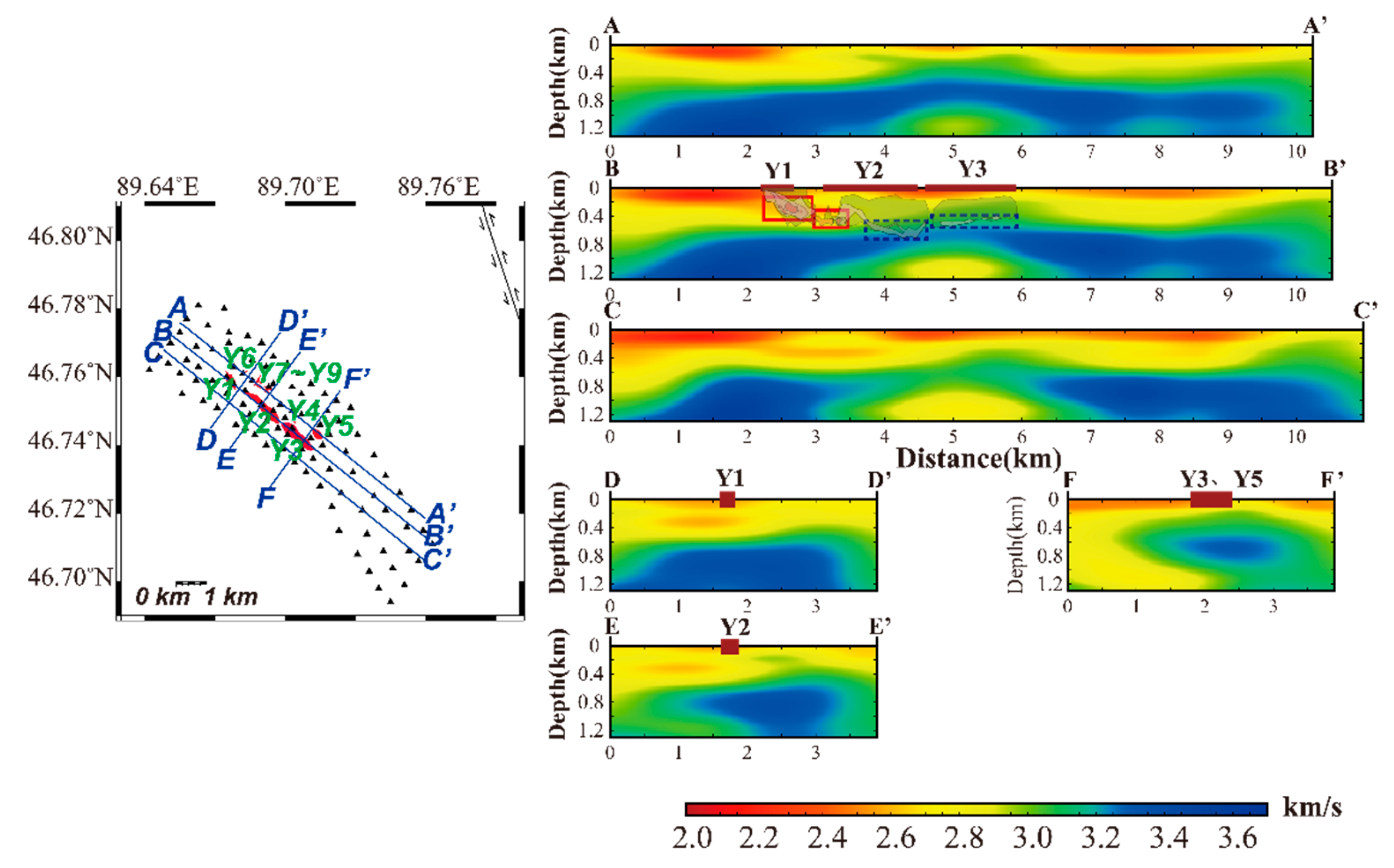
Figure 9.
Vertical profiles of shear wave velocity and distribution of ore-body intrusions. Left: Surface distribution of ore-hosting intrusions and location of the profiles. Black triangles are station of KMA. Red areas are ore-hosting intrusions Y1~Y9 with names labeled in green. Along profile in B-B′, D-D′, E-E′ and F-F′ ore hosting intrusions are marked at the surface. Along B-B′ the transparent zones with black lines are ore hosting intrusions with different mineralization [5]. Red solid rectangles along B-B′ represent LVZs at Y1 and northwest of Y2, which have highest degree of mineralization. Blue dotted rectangles include HVZs southeast of Y2 and Y3, which have lower degree of mineralization.

Figure 10.
Horizontal resolution tests of numbers of stations. The left panel shows the synthetic model. (a–c) the model recoveries with 50 stations at depth of 0.1, 0.5 and 0.85 km in order. (d–f) the model recoveries with 70 stations at depth of 0.1, 0.5 and 0.85 km in order. (g–i) the model recoveries with 90 stations at depth of 0.1, 0.5 and 0.85 km in order. (j–l) the model recoveries with 100 stations at depth of 0.1, 0.5 and 0.85 km in order.

Figure 11.
Potential of geophysical models in aiding deep prospecting work. (a) Surface distribution of orebodies. (b) Magnetic and gravity anomalies from [5]. (c) Locations of intrusions along the NW–SE profile across the three main ore bodies Y1 to Y3. The shapes of the intrusions were determined by drilling data from [5]. Red boxes are highly mineralized intrusions and blue boxes are much less mineralized. (d) Velocity model from ambient noise inversion.

© 2020 by the authors. Licensee MDPI, Basel, Switzerland. This article is an open access article distributed under the terms and conditions of the Creative Commons Attribution (CC BY) license (http://creativecommons.org/licenses/by/4.0/).
Share and Cite
MDPI and ACS Style
Du, P.; Wu, J.; Li, Y.; Wang, J.; Han, C.; Lindsay, M.D.; Yuan, H.; Zhao, L.; Xiao, W. Imaging Karatungk Cu-Ni Mine in Xinjiang, Western China with a Passive Seismic Array. Minerals 2020, 10, 601. https://doi.org/10.3390/min10070601
AMA Style
Du P, Wu J, Li Y, Wang J, Han C, Lindsay MD, Yuan H, Zhao L, Xiao W. Imaging Karatungk Cu-Ni Mine in Xinjiang, Western China with a Passive Seismic Array. Minerals. 2020; 10(7):601. https://doi.org/10.3390/min10070601
Chicago/Turabian StyleDu, Peixiao, Jing Wu, Yang Li, Jian Wang, Chunming Han, Mark Douglas Lindsay, Huaiyu Yuan, Liang Zhao, and Wenjiao Xiao. 2020. "Imaging Karatungk Cu-Ni Mine in Xinjiang, Western China with a Passive Seismic Array" Minerals 10, no. 7: 601. https://doi.org/10.3390/min10070601
Note that from the first issue of 2016, this journal uses article numbers instead of page numbers. See further details here.