Exact Values of the Gamma Function from Stirling’s Formula

Abstract

In this work the complete version of Stirling’s formula, which is composed of the standard terms and an infinite asymptotic series, is used to obtain exact values of the logarithm of the gamma function over all branches of the complex plane. Exact values can only be obtained by regularization. Two methods are introduced: Borel summation and Mellin–Barnes (MB) regularization. The Borel-summed remainder is composed of an infinite convergent sum of exponential integrals and discontinuous logarithmic terms that emerge in specific sectors and on lines known as Stokes sectors and lines, while the MB-regularized remainders reduce to one complex MB integral with similar logarithmic terms. As a result that the domains of convergence overlap, two MB-regularized asymptotic forms can often be used to evaluate the logarithm of the gamma function. Though the Borel-summed remainder has to be truncated, it is found that both remainders when summed with (1) the truncated asymptotic series, (2) Stirling’s formula and (3) the logarithmic terms arising from the higher branches of the complex plane yield identical values for the logarithm of the gamma function. Where possible, they also agree with results from Mathematica.

1. Introduction

Discovered in the 1730s [1], Stirling’s formula is a well-known result for determining approximate values of the gamma function, $\mathsf{\Gamma }\left(z\right)$, which is so important in the definition of Mittag–Leffler functions. Mystery has lingered whether it is indeed possible to obtain exact values of the gamma function from the complete version of the formula as opposed to its more famous truncated form. Moreover, due to the function’s rapid exponentiation, its logarithm or $ln\mathsf{\Gamma }\left(z\right)$ is studied more often. This, however, introduces multivaluedness, which makes the asymptotic analysis of the function more formidable. Consequently, no one has ever been able to obtain exact values of either function via the entire formula.

In its entirety, Stirling’s formula is an asymptotic expansion and is, therefore, divergent. Here exact values of $ln\mathsf{\Gamma }\left(z\right)$ are determined for all values of $argz$ from the complete asymptotic expansion of the formula. This process known as exactification represents the ultimate goal of hyperasymptotics, whose primary aim is to obtain far more accurate values from asymptotic expansions than standard Poincaré asymptotics [2]. In such studies one not only includes all the terms in a dominant asymptotic series, but also, subdominant exponential terms, which are said to lie beyond all orders [3]. To observe their effect, hyperasymptotic calculations are generally carried out to more than 20 decimal places.

Since a complete asymptotic expansion is composed of divergent series, exactification involves obtaining meaningful values from them. This is achieved by the process of regularization, which is defined here as the removal of the infinity in the remainder of an asymptotic series so as to make the series summable. It was first demonstrated in [4] that the infinity in the remainder of an asymptotic series arises from an impropriety in the asymptotic method used to derive it. Hence regularization represents the method of correcting asymptotic methods.

Two very different techniques will be used to regularize the divergent series in this work. As discussed in [5,6], the most common method of regularizing a divergent series is Borel summation, but often, it produces results that are not amenable to fast and accurate computation. To overcome this drawback, the numerical technique of Mellin–Barnes regularization was developed in [7]. In this method, divergent series are expressed in terms of Mellin–Barnes integrals and divergent arc-contour integrals. Regularization removes the latter resulting in the Mellin–Barnes integrals yielding finite values, similar to the Hadamard finite part of a divergent integral [8]. Amazingly, the finite values obtained from applying the technique to an asymptotic expansion yield exact values of the original function with the main difference being that instead of dealing with Stokes sectors and lines, one now deals with overlapping domains of convergence over which the Mellin–Barnes integrals are valid.

2. Stirling’s Formula

Stirling’s formula [1] for the factorial function is often written for large integers, n, as

$$\begin{array}{c}\hfill lnn!=ln\mathsf{\Gamma }(n+1)=nlnn-n+\frac{1}{2}ln\left(2\pi n\right)+\cdots .\end{array}$$

(1)

As this is accurate to within 1% for $n>5$, it represents a good approximation in standard (Poincaré) asymptotics [2], but not so in hyperasymptotics. Moreover, our aim is to consider complex values, not large integers. Thus, we replace the factorial function by the more general gamma function, $\mathsf{\Gamma }(z+1)$. The terms in (1), denoted here by $F\left(z\right)$, then become the leading terms of the complete asymptotic expansion for $ln\mathsf{\Gamma }\left(z\right)$. They will be treated as a separate contribution in all calculations of $ln\mathsf{\Gamma }\left(z\right)$, so that the reader will be able to observe just how inadequate standard asymptotics is compared with hyperasymptotics.

Occasionally, a problem arises where there is an interest in the missing terms in (1). Then Stirling’s formula is expressed differently. For example, according to No. 6.1.41 in [9], for $z\to \infty$ and $\left|\arg z\right|<\pi$, $ln\mathsf{\Gamma }\left(z\right)$ is given by

$$\begin{array}{c}\hfill ln\mathsf{\Gamma }\left(z\right)\sim F\left(z\right)+\frac{1}{12z}-\frac{1}{360z^3}+\frac{1}{1260z^5}-\frac{1}{1680z^7}+\cdots ,\end{array}$$

(2)

where $F\left(z\right)$ represents all the terms in Stirling’s formula, namely,

$$\begin{array}{c}\hfill F\left(z\right)=\left(z-\frac{1}{2}\right)lnz-z+\frac{1}{2}ln\left(2\pi \right).\end{array}$$

(3)

Hence the leading terms are identical to those in (1). In other texts the dots in (2) are replaced by the Landau gauge symbol, which would be $O\left(z^{-9}\right)$ here since it is the next highest order term. In [10] the power series after $ln\left(2\pi \right)$ is truncated with the coefficients expressed in terms of the Bernoulli numbers, while the remainder term, $R_N\left(z\right)$ in No. 8.344, is given as

$$\begin{array}{c}\hfill \left|R_N\left(z\right)\right|=\left|\sum _{k=N}^{\infty }\frac{B_{2k}}{2k(2k-1)z^{2k-1}}\right|<\frac{|B_{2n}|}{{2n(2n-1)\left|z\right|}^{2n-1}{cos}^{2n-1}((argz)/2)}.\end{array}$$

(4)

Although the remainder is dependent upon z and N, for $\Re z>0$, the series diverges once N passes the optimal point of truncation, $N_{OP}$. Moreover, the above result is even more vague than (2) because the expansion is only valid for “large” values of $\left|z\right|$ without indicating what large means. Here, we shall evaluate exact values of $ln\mathsf{\Gamma }\left(z\right)$ from the complete version of Stirling’s formula by following the concepts and theory in [6], but before this can be done, the following lemma is required.

Lemma 1.

Via regularization, the power/Taylor series expansion for $\arctan u$, namely, ${\sum }_{k=0}^{\infty }{u}^{2k+1}/(2k+1)$, can be expressed as

$$\begin{array}{c}\hfill \sum _{k=0}^{\infty }\frac{{(-1)}^k{u}^{2k+1}}{(2k+1)}\left\{\begin{array}{cc}=\arctan u,\hfill & -1<\Re \left(iu\right)<1,\hfill \\ \equiv \arctan u,\hfill & \Re \left(iu\right)\le -1,\mathrm{and}\Re \left(iu\right)\ge 1.\hfill \end{array}\right.\end{array}$$

(5)

Proof. 

For brevity, the proof is not given here, but appears in [11]. □

It should be noted that an equivalence symbol appears in one of the results, indicating that one side possesses a divergent series, while the other side represents a finite regularized value. That is, $\arctan ,\mathrm{u}$ is defined for all values of u, while the series representation for the function is divergent when u does not lie within $-1<\Re \left(iu\right)<1$. Since the equivalence symbol is less stringent than an equals sign, we can re-write the lemma as

$$\begin{array}{c}\hfill \sum _{k=0}^{\infty }\frac{{(-1)}^k{u}^{2k+1}}{(2k+1)}\equiv \arctan u,\forall u.\end{array}$$

(6)

Therefore, if the series appears in a problem, then it can be replaced by the right-hand side (rhs). Though equivalence statements will appear throughout this paper, it does not necessarily mean that a power series is divergent for all values of the variable.

Now we derive the complete form of Stirling’s formula. This will not be original, but we need to establish that it is complete. Binet’s second expression for $ln\mathsf{\Gamma }\left(z\right)$ in [2] is

$$\begin{array}{c}\hfill ln\mathsf{\Gamma }\left(z\right)=F\left(z\right)+2{\int }_0^{\infty }dt\frac{\arctan (t/z)}{e^{2\pi t}-1}.\end{array}$$

(7)

By making a change of variable, $y=2\pi t$, and noting that z is complex, we can then introduce (5). Replacing k by $k+1$ yields

$$\begin{array}{c}\hfill ln\mathsf{\Gamma }\left(z\right)-F\left(z\right)\equiv \frac{1}{\pi }\sum _{k=1}^{\infty }\frac{{(-1)}^{k+1}}{(2k-1)}{\left(\frac{1}{2\pi z}\right)}^{2k-1}{\int }_0^{\infty }dy\frac{y^{2k-1}}{e^y-1}.\end{array}$$

(8)

The left-hand side (lhs) of (8) is finite (convergent), while the rhs can be either divergent or convergent. From No. 3.411(1) in [10], the integral in the above equivalence is equal to $\mathsf{\Gamma }\left(2k\right)\zeta \left(2k\right)$, where $\zeta \left(z\right)$ represents the Riemann zeta function. Thus, the above result becomes

$$\begin{array}{c}\hfill ln\mathsf{\Gamma }\left(z\right)-F\left(z\right)\equiv 2z\sum _{k=1}^{\infty }\frac{{(-1)}^{k+1}}{(2k-1)}\frac{\mathsf{\Gamma }\left(2k\right)\zeta \left(2k\right)}{{\left(2\pi z\right)}^{2k}}.\end{array}$$

(9)

From here on, $S\left(z\right)$ denotes the series on the rhs. On the other hand, Paris and Kaminski [12,13], replace the terms on the lhs by $\mathsf{\Omega }\left(z\right)$. With the aid of the reflection formula for the gamma function, the following continuation formula can be derived:

$$\begin{array}{c}\hfill \mathsf{\Omega }\left(z\right)+\mathsf{\Omega }\left(z{e}^{\pm i\pi }\right)=-ln\left(1-e^{\mp 2i\pi z}\right).\end{array}$$

(10)

This enables one to obtain values of $ln\mathsf{\Gamma }\left(z\right)$ whenever z is situated in the left-hand complex plane via the corresponding values in the right-hand complex plane. Furthermore, the rhs will play an important role when the Stokes phenomenon is discussed later.

In order to continue with this study, the following definitions are required:

Definition 1.

An asymptotic (power) series is defined here as an infinite power series with zero radius of absolute convergence.

Definition 2.

An asymptotic form is composed of: (1) a complete asymptotic expansion, which not only possesses all terms in a dominant asymptotic power series, e.g., $S\left(z\right)$ above, but also all the terms in each subdominant asymptotic series, should they exist, and (2) the common sector or ray in the complex plane over which the argument of the variable in each series is valid.

By truncating $S\left(z\right)$ at N terms, we arrive at

$$\begin{array}{c}\hfill S\left(z\right)=z\sum _{k=1}^{N-1}\frac{{(-1)}^k}{{\left(2z\right)}^{2k}}\mathsf{\Gamma }(2k-1)c_k\left(1\right)-2z\sum _{n=1}^{\infty }\sum _{k=N}^{\infty }\frac{{(-1)}^k}{{\left(2\pi nz\right)}^{2k}}\mathsf{\Gamma }(2k-1),\end{array}$$

(11)

where the first term will be denoted as $T{S}_N\left(z\right)$, N is the truncation parameter and $c_k\left(1\right)$ represents a specific value of the cosecant polynomials [14], given by

$$\begin{array}{c}\hfill c_k\left(1\right)=-2\zeta \left(2k\right)/{\pi }^{2k}.\end{array}$$

(12)

The infinite series over k in the second term is known as a generalized Type I terminant [6]. Terminants were first introduced by Dingle [15] because he found that special functions often possess asymptotic series whose late coefficients exhibit gamma function growth, viz. $\mathsf{\Gamma }(k+\alpha )$. A Type II terminant differs in that the coefficients possess an extra phase factor of ${(-1)}^k$.

The notation $S_{p,q}^I(N,z^{\beta })$ was introduced in [6] to denote the generalization of Dingle’s Type I terminants, which are defined as

$$\begin{array}{c}\hfill S_{p,q}^I\left(N,z^{\beta }\right)\doteqdot \sum _{k=N}^{\infty }{(-1)}^k\mathsf{\Gamma }(pk+q)z^{\beta k}.\end{array}$$

(13)

Alternatively, (11) can be expressed as

$$\begin{array}{c}\hfill S\left(z\right)=z\sum _{k=1}^{N-1}\frac{{(-1)}^k}{{\left(2z\right)}^{2k}}\mathsf{\Gamma }(2k-1)c_k\left(1\right)-2z\sum _{n=1}^{\infty }{S}_{2,-1}^I\left(N,{(1/2n\pi z)}^2\right).\end{array}$$

(14)

Thus, $\beta$ and z in (13) are equal to 2 and $1/2n\pi z$ in (14). Although [6] states that both p and q have to be positive and real, it is $N+q/p$, which appears in the regularized value of a generalized terminant. Therefore, provided $\Re (N+q/p)>0$, the regularized value of the series still exists. Alternatively, k can be replaced by $k+1$ in the infinite series in (14), in which case q equals unity. Since $S_{2,-1}^I\left(N,z^2\right)=-z^2{S}_{2,1}^I\left(N-1,z^2\right)$, we can apply the result in [6] to $S_{2,1}^I\left(N-1,z^2\right)$ instead.

According to Rule A in ([15], Chapter 1), Stokes lines occur whenever the arguments or phases of the variable result in the terms of an asymptotic series becoming homogeneous in phase and having the same sign. In the case of the generalized terminant in (13), this means that Stokes lines occur whenever $\arg \left(-z^{\beta }\right)=2l\pi$, for l, an integer. Then the terms in either $S_{2,-1}^I(N,1/z^2)$ or $S_{2,1}^I(N,1/z^2)$ are all positively real. Because l is arbitrary, we can replace $-1$ by $exp(-i\pi )$. Thus, we find that the Stokes lines for $S\left(z\right)$ occur whenever $\arg z=-(l+1/2)\pi$, i.e., at half integer multiples of $\pi$.

The concept of a primary Stokes sector/line was introduced in [6] to indicate the first Stokes sector/line over which an asymptotic expansion is derived. It was also necessary to define asymptotic forms since two functions can have the same complete asymptotic expansion, but will still be different if the expansion applies over different primary Stokes sectors or lines. For example, in solving a problem for positive real values of the variable, one may obtain a generalized Type I terminant as the asymptotic solution. However, as the variable moves off the real axis, it will acquire subdominant semi-residue contributions of opposing signs in either direction as a result of the Stokes phenomenon. However, if the same asymptotic solution is obtained for positive imaginary values of the variable, then as the variable hits the positive and negative real axes, the asymptotic solution will acquire a semi-residue contribution. When the variable moves into the lower half of the complex plane, the asymptotic solution will acquire a full residue contribution. Clearly, both cases are different and will yield different values even though the same generalized Type I terminant was derived. Hence the original functions or solutions for these cases are different. In the first case the positive real axis becomes the primary Stokes line for the generalized Type I terminant, while in the second case, the upper half of the complex plane represents the primary Stokes sector. Then as more secondary Stokes sectors/lines are encountered either in a clockwise or anti-clockwise direction from the primary Stokes sector/line, more Stokes discontinuities arise at the boundaries. Although the choice of a primary Stokes sector/line is arbitrary, it will be taken here to be the Stokes sector/line situated in the principal branch of the complex plane, since most asymptotic expansions are derived under the condition that the variable lies initially in the principal branch of the complex plane.

Before we can regularize the asymptotic series, $S\left(z\right)$, we require the following lemma:

Lemma 2.

Regularization of the Taylor series for the logarithmic function yields

$$\begin{array}{c}\hfill \sum _{k=1}^{\infty }\frac{{(-1)}^{k+1}}{k}{z}^k\left\{\begin{array}{cc}\equiv ln(1+z),\hfill & \Re z\le -1,\hfill \\ =ln(1+z),\hfill & \Re z>-1.\hfill \end{array}\right.\end{array}$$

(15)

Proof. 

There is no need for the proof to appear here as it can be found in [16]. □

As in the first lemma, we can replace the equals sign in the lemma by the less stringent equivalence symbol, which reduces the lemma to

$$\begin{array}{c}\hfill \sum _{k=1}^{\infty }\frac{{(-z)}^k}{k}\equiv -ln(1+z),\forall z.\end{array}$$

(16)

With this result we can now regularize $S\left(z\right)$, which will enable the asymptotic forms for $ln\mathsf{\Gamma }\left(z\right)$ to be derived.

Theorem 1.

As a result of the regularization of its asymptotic power series, the logarithm of the gamma function possesses the following asymptotic forms:

$$ln\mathsf{\Gamma }\left(z\right)=F\left(z\right)+z\sum _{k=1}^{N-1}\frac{{(-1)}^k}{{\left(2z\right)}^{2k}}\mathsf{\Gamma }(2k-1)c_k\left(1\right)+R_N^{SS}\left(z\right)+S{D}_M^{SS}\left(z\right),$$

(17)

where the remainder $R_N^{SS}\left(z\right)$ is given by

$$\begin{array}{cc}\hfill R_N^{SS}\left(z\right)& =\frac{2{(-1)}^{N+1}z}{{\left(2\pi z\right)}^{2N}}{\int }_0^{\infty }dy{y}^{2N-2}{e}^{-y}\sum _{n=1}^{\infty }\frac{1}{n^{2N-2}\left({(y/2\pi z)}^2+n^2\right)},\hfill \end{array}$$

(18)

and the Stokes discontinuity term $S{D}_M\left(z\right)$ is given by

$$\begin{array}{cc}\hfill S{D}_M^{SS}\left(z\right)& =-\lfloor M/2\rfloor ln\left(-e^{\pm 2i\pi z}\right)-\frac{\left(1-{(-1)}^M\right)}{2}ln\left(1-e^{\pm 2i\pi z}\right).\hfill \end{array}$$

(19)

The remainder is valid for either $(M-1/2)\pi <\theta =\arg z<(M+1/2)\pi$ or $-(M+1/2)\pi <\theta <-(M-1/2)\pi$, where M is a non-negative integer. However, the Stokes discontinuity term possesses two forms that are complex conjugates. The upper-signed version of (19) applies to $(M-1/2)\pi <\theta <(M+1/2)\pi$, while the lower-signed version is valid over $-(M+1/2)\pi <\theta <-(M-1/2)\pi$. For z lying on the Stokes lines, i.e., for $\theta =\pm (M+1/2)\pi$, $R_N^{SS}\left(z\right)$ and $S{D}_M^{SS}\left(z\right)$ are replaced by $R_N^{SL}\left(z\right)$ and $S{D}_M^{SL}\left(z\right)$, respectively. Then the remainder is given by

$$\begin{array}{cc}\hfill R_N^{SL}\left(z\right)& =\frac{2z}{{\left(2\pi \right|z\left|\right)}^{2N-2}}P{\int }_0^{\infty }dy{y}^{2N-2}{e}^{-y}\sum _{n=1}^{\infty }\frac{1}{n^{2N-2}(y^2-4n^2{\pi }^2{\left|z\right|}^2)},\hfill \end{array}$$

(20)

while the Stokes discontinuity term becomes

$$\begin{array}{cc}\hfill S{D}_M^{SL}\left(z\right)& ={(-1)}^M\left(\lfloor M/2\rfloor +\frac{1-{(-1)}^M}{2}\right)2\pi \left|z\right|-\frac{1}{2}ln\left(1-e^{-2\pi \left|z\right|}\right).\hfill \end{array}$$

(21)

In (20), P denotes the Cauchy principal value.

Proof. 

For brevity, the proof is not presented here as it can be found in [11]. □

The remainder in Theorem 1 is conceptually different from the remainder term in standard Poincaré asymptotics, which is expressed in terms of the Landau gauge symbol, $\mathcal{O}\left(\right)$, or as $+\cdots$ In fact, (17) would typically be written as

$$\begin{array}{c}\hfill ln\mathsf{\Gamma }\left(z\right)=F\left(z\right)-\frac{c_1\left(1\right)}{4z}+\frac{c_2\left(1\right)}{8z^3}-\frac{3c_3\left(1\right)}{8z^5}+\mathcal{O}\left(\frac{1}{z^7}\right).\end{array}$$

(22)

Moreover, by introducing $c_1\left(1\right)=-1/3$, $c_2\left(1\right)=-1/45$, $c_3\left(1\right)=-2/945$ and $c_4\left(1\right)=-1/4725$, into the above result, we obtain (2). For real values of z, (22) is referred to as a large z or $z\to \infty$ expansion with the limit point at infinity. For z complex, it becomes a large $\left|z\right|$ expansion. In other cases, where the Landau gauge symbol is omitted, a tilde often replaces the equals sign. Nevertheless, in all these representations it means that the later terms in the truncated power series have been neglected despite their eventual divergence past the optimal point of truncation.

3. Numerical Analysis

In the previous section the asymptotic forms for $ln\mathsf{\Gamma }\left(z\right)$ were derived via Borel summation. However, we still need to verify that these results yield exact values of the special function. This section aims to present such a numerical analysis. For the analysis to be effective, a large number of values of $\left|z\right|$ is not required. This is because the results change across Stokes sectors or rays, but within each sector or on each line, they behave uniformly with respect to z. Thus, a few values of $\left|z\right|$ are necessary for testing the validity of the asymptotic forms. In fact, only two values of $\left|z\right|$ are necessary: a relatively large one, where the asymptotic series in (17) can be truncated, and a small one, where truncation breaks down completely. Then a range of values for both N and $\arg z$ or $\theta$, need to be considered across the Stokes sectors and lines. Note also that selecting extremely large/small values of $\left|z\right|$ may result in overflow or underflow problems in the numerical calculations. This would then give the misleading impression that the asymptotic forms are incorrect rather than implying a deficiency in the computing system. Since the variable in the asymptotic series is $1/{\left(2n\pi z\right)}^2$ with n ranging from unity to infinity, $\left|z\right|=3$ is deemed to be sufficiently large, while for $\left|z\right|=1/10$, there is no optimal point of truncation. The second value is, therefore, sufficiently small to demonstrate the breakdown of standard Poincaré asymptotics.

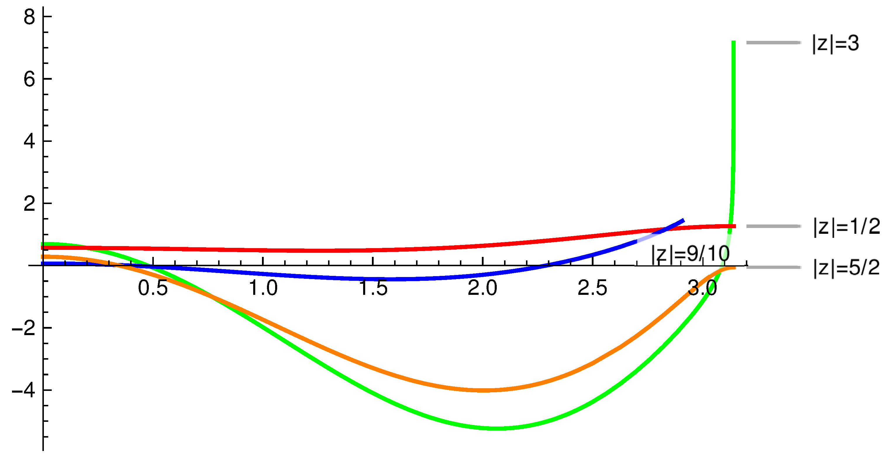
Before undertaking the numerical analysis, let us present plots of $ln\mathsf{\Gamma }\left(z\right)$ to help the reader understand the nature of the function. Figure 1 displays graphs of the real part of the function for several fixed values of $\left|z\right|$ used in this paper as a function of $\theta$ over $(0,\pi )$. There we see for the larger values of $\left|z\right|$, the real part of $ln\mathsf{\Gamma }\left(z\right)$ dips to a minimum before it begins to grow dramatically, which is the rapid exponentiation mentioned in the introduction. The smaller values of $\left|z\right|$ do not vary as much, although both are similar to the larger values of $\left|z\right|$ in that they dip to a minimum and rise afterwards. Unlike the other graphs, the graph for $\left|z\right|=1/2$ has a positive minimum and increases rather slowly.

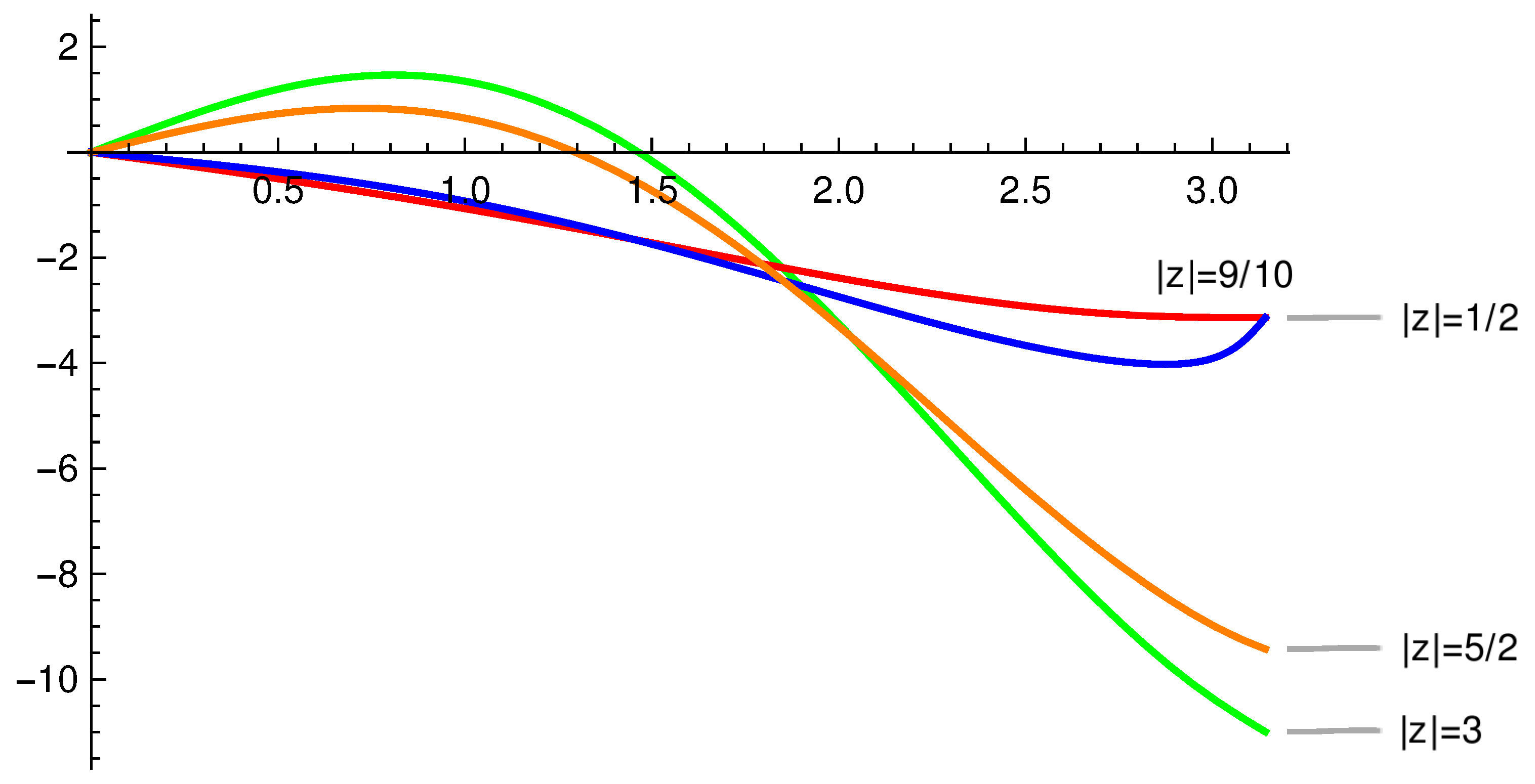
Figure 2 displays graphs of the imaginary part of $ln\mathsf{\Gamma }\left(z\right)$ for the same fixed values of $\left|z\right|$ as a function of $\theta$ over $(0,\pi )$. Here we see that the large values of $\left|z\right|$ rise to a positive maximum before rapidly decreasing into the negative right quadrant. The plot for $\left|z\right|=9/10$ does not attain a positive maximum, but decreases relatively slowly from the origin into the negative right quadrant. The graph for $\left|z\right|=1/2$ follows that for $\left|z\right|=9/10$ until about $\theta =\pi /2$. Then it decreases faster than the $\left|z\right|=9/10$ graph, but when $\theta$ is close to $\pi$, it rises until it meets the $\left|z\right|=9/10$ graph at $\theta =\pi$.

The optimal point of truncation, $N_{OP}$, is determined by calculating the first value of the truncation parameter, N, when successive terms in an asymptotic series begin to dominate the preceding terms. That is, it occurs at the first value of k, where the $k+1$-th term is greater than the k-th term in $S\left(z\right)$, namely,

$$\begin{array}{c}\hfill \left|\frac{2k(2k-1)}{{\left(2z\right)}^2}\frac{c_{k+1}\left(1\right)}{c_k\left(1\right)}\right|=\left|\frac{2k(2k-1)}{{\left(2\pi z\right)}^2}\frac{\zeta (2k+2)}{\zeta \left(2k\right)}\right|\approx 1.\end{array}$$

(23)

Since the ratio of the Riemann zeta functions is close to unity, we observe that $N_{OP}$ occurs around $\pi \left|z\right|$. Therefore, for $\left|z\right|=3$, $N_{OP}$ will be close to 10, while for $\left|z\right|=1/10$, it does not exist, meaning that $N_{OP}=0$. In the latter case the first or leading term of the asymptotic series will yield the “nearest” value to $ln\mathsf{\Gamma }\left(z\right)$, but it will not be accurate. On the other hand, the larger $N_{OP}$ is, the more accurate truncation of the asymptotic series becomes.

Typically, when a software package such as Mathematica [17] determines values of a special function, it only does so over the principal branch of the complex plane. Hence, the numerical analysis will be confined to $\arg z$ over $(-\pi ,\pi ]$, which means in turn that the numerical analysis of (17) will only be conducted over the three Stokes sectors, $-3\pi /2<\theta <-\pi /2$, $-\pi /2<\theta <\pi /2$ and $\pi /2<\theta <3\pi /2$, and the two Stokes lines at $\theta =\pm \pi /2$. In other words, only the $M=0$ and $M=\pm 1$ results in Theorem 1 will be tested for the time being. By denoting the truncated sum in (17) by $T{S}_N\left(z\right)$, i.e.,

$$\begin{array}{c}\hfill T{S}_N\left(z\right)=z\sum _{k=1}^{N-1}\frac{{(-1)}^k}{{\left(2z\right)}^{2k}}\mathsf{\Gamma }(2k-1)c_k\left(1\right),\end{array}$$

(24)

we need to verify the following results:

$$\begin{array}{c}\hfill ln\mathsf{\Gamma }\left(z\right)=\left\{\begin{array}{cc}F\left(z\right)+T{S}_N\left(z\right)+R_N^{SS}\left(z\right)+S{D}_1^{SS,U}\left(z\right),\hfill & \pi /2<\theta \le \pi ,\hfill \\ F\left(z\right)+T{S}_N\left(z\right)+R_N^{SL}\left(z\right)+S{D}_0^{SL}\left(z\right),\hfill & \theta =\pi /2,\hfill \\ F\left(z\right)+T{S}_N\left(z\right)+R_N^{SS}\left(z\right),\hfill & -\pi /2<\theta <\pi /2,\hfill \\ F\left(z\right)+T{S}_N\left(z\right)+R_N^{SL}\left(z\right)+S{D}_0^{SL}\left(z\right),\hfill & \theta =-\pi /2,\hfill \\ F\left(z\right)+T{S}_N\left(z\right)+R_N^{SS}\left(z\right)+S{D}_1^{SS,L}\left(z\right),\hfill & -\pi <\theta <-\pi /2.\hfill \end{array}\right.\end{array}$$

(25)

In the above the superscripts, U and L, have been introduced into the Stokes discontinuity terms in the Stokes sectors to indicate the upper- and lower-signed versions of (21). Although equal to zero, the Stokes discontinuity term for the third asymptotic form will be denoted as $S{D}_0^{SS}\left(z\right)$.

If we put $N=4$ in the third result of (24) and neglect the final term or remainder, then we arrive at (2). However, the remaining terms in this result are now expressed as

$$\begin{array}{cc}\hfill R_N^{SS}\left(z\right)& =\frac{2{(-1)}^{N+1}z}{{\left(2\pi z\right)}^{2N-2}}\sum _{n=1}^{\infty }\frac{1}{n^{2N-2}}{\int }_0^{\infty }dy\frac{y^{2N-2}{e}^{-y}}{\left(y^2+4{\pi }^2{n}^2{z}^2\right)},\hfill \end{array}$$

(26)

and

$$\begin{array}{cc}\hfill R_N^{SL}\left(z\right)& =\frac{2z}{{\left(2\pi \right|z\left|\right)}^{2N-2}}\sum _{n=1}^{\infty }\frac{1}{n^{2N-2}}P{\int }_0^{\infty }dy\frac{y^{2N-2}{e}^{-y}}{\left(y^2-4{\pi }^2{n}^2{\left|z\right|}^2\right)},\hfill \end{array}$$

(27)

while the Stokes discontinuity terms are given by

$$\begin{array}{c}\hfill S{D}_1^{SS}\left(z\right)=-ln\left(1-e^{\pm 2\pi zi}\right),\end{array}$$

(28)

and

$$\begin{array}{c}\hfill S{D}_0^{SL}\left(z\right)=-\frac{1}{2}ln\left(1-e^{-2\pi \left|z\right|}\right).\end{array}$$

(29)

Note the connection with $\mathsf{\Omega }\left(z\right)$ mentioned below (9).

For the numerical analysis we need to consider the results over the Stokes sectors separately from those at the Stokes lines since the latter require the evaluation of the Cauchy principal value and the Stokes discontinuity terms possess a factor of $1/2$ compared with zero when $\left|\theta \right|<\pi /2$ or unity when $\left|\theta \right|>\pi /2$. Thus, $ln\mathsf{\Gamma }\left(z\right)$ will be evaluated via two different Mathematica modules: one involving the standard numerical integration routine called NIntegrate, and another, where NIntegrate is adapted to evaluate only the Cauchy principal value.

When $\theta >0$, the Stokes discontinuity terms can be combined into one expression, denoted by $S{D}^{+}\left(z\right)$. This is given by

$$\begin{array}{c}\hfill S{D}^{+}\left(z\right)=-S^{+}ln\left(1-e^{2\pi iz}\right),\end{array}$$

(30)

where the Stokes multiplier, $S^{+}$, is written as

$$\begin{array}{c}\hfill S^{+}=\left\{\begin{array}{cc}1,\hfill & \pi /2<\theta \le \pi ,\hfill \\ 1/2,\hfill & \theta =\pi /2,\hfill \\ 0,\hfill & -\pi /2<\theta <\pi /2.\hfill \end{array}\right.\end{array}$$

(31)

Similarly, the Stokes discontinuity terms in the lower half of the principal branch, $S{D}^{-}\left(z\right)$, can be written in terms of another Stokes multiplier, $S^{-}$, as follows:

$$\begin{array}{c}\hfill S{D}^{-}\left(z\right)=S^{-}ln\left(1-e^{-2\pi iz}\right),\end{array}$$

(32)

where $S^{-}$ is given by

$$\begin{array}{c}\hfill S^{-}=\left\{\begin{array}{cc}0,\hfill & -\pi /2<\theta <\pi /2,\hfill \\ 1/2,\hfill & \theta =-\pi /2,\hfill \\ 1,\hfill & -\pi <\theta <-\pi /2.\hfill \end{array}\right.\end{array}$$

(33)

From the above, we see that the Stokes multipliers are discontinuous, which is known as the conventional view of the Stokes phenomenon. However, an alternative view of the Stokes phenomenon arose in the late 1980s where they were no longer regarded as step-functions. Instead, it was proposed that they undergo a smooth, but rapid, transition from zero to unity, equalling $1/2$ at the Stokes line [18]. Today, this is known as Stokes smoothing, despite the fact that Stokes never regarded the multipliers as being smooth [19]. According to this approach, first put forward by Berry and then made more “rigorous” by Olver [20], the Stokes multiplier reduces to the error function, $\mathrm{erf}\left(z\right)$. Later, Berry [21] and Paris and Wood [22] found an approximate form for the Stokes multipliers of $ln\mathsf{\Gamma }\left(z\right)$, which were given as

$$\begin{array}{c}\hfill S^{\pm }\left(z\right)\sim \frac{1}{2}\pm \frac{1}{2}\mathrm{erf}\left((\theta \pm \pi /2)\sqrt{\pi \left|z\right|}\right).\end{array}$$

(34)

A graph of (34) for $\left|z\right|=3$ versus $\theta$ is displayed in Figure 3 together with the conventional view or (31). For $\theta <1$, (34) is virtually zero, while for $\theta >2$, it is almost equal to unity. In between, however, the rapid smoothing occurs with the greatest deviation from the step-function occurring in the vicinity of the Stokes line where both views possess a common (green) point at ($\pi$/2, 1/2). If smoothing occurs, then Theorem 1 cannot possibly yield exact values of $ln\mathsf{\Gamma }\left(z\right)$, especially for $\theta$ between $13\pi /32$ and $17\pi /32$ excluding $\pi /2$.

We can establish the correct view by calculating $ln\mathsf{\Gamma }\left(z\right)$ for $\theta$ between $13\pi /32$ and $17\pi /32$ using (30) since smoothing implies that (30) cannot possibly yield exact values of $ln\mathsf{\Gamma }\left(z\right)$. However, if we obtain exact values of $ln\mathsf{\Gamma }\left(z\right)$, then we know that the conventional view holds and smoothing is a fallacy. The problem with testing (34) directly is that it applies to much larger values of $\left|z\right|$ than 3. The proponents of smoothing have not provided the form for smaller values of $\left|z\right|$. For very large values of $\left|z\right|$, truncating the asymptotic expansion at a few terms will yield very accurate values for $ln\mathsf{\Gamma }\left(z\right)$, which can obscure both views unless an extremely high precision and time-consuming analysis is undertaken. Hence much smaller values of $\left|z\right|$ will be considered in (30), so that the Stokes discontinuity term can no longer be neglected.

Before Stokes smoothing can be investigated, we must show that (24) behaves as a typical asymptotic expansion. That is, we must show that for large values of $\left|z\right|$, the remainder can be neglected to yield accurate, but nevertheless approximate, values of $ln\mathsf{\Gamma }\left(z\right)$ up to and not very far from the optimal point of truncation, while for small values of $\left|z\right|$, it is simply invalid to neglect the remainder. For this demonstration we do not require the Stokes discontinuity terms. Thus, we shall study the asymptotic series for $\left|\theta \right|<\pi /2$, in particular $\theta =0$, because it does not require complex arithmetic.

From (26) we see that the evaluation of the remainder involves two computationally intensive tasks. The first is the infinite sum over n, which arose due to an infinite number of singularities lying on each Stokes line. The second issue is the numerical integration of the exponential integral. The latter can be avoided by decomposing the denominator into partial fractions and using No. 3.383(10) from [10]. For $\left|\theta \right|<\pi /2$, one then obtains

$$\begin{array}{cc}\hfill R_N^{SS}\left(z\right)& =\frac{\mathsf{\Gamma }(2N-1)}{2\pi i}\sum _{n=1}^{\infty }\frac{1}{n}(e^{-2\pi nzi}\mathsf{\Gamma }(2-2N,-2\pi nzi)\hfill \\ \hfill & -e^{2\pi nzi}\mathsf{\Gamma }(2-2N,2\pi nzi)).\hfill \end{array}$$

(35)

The above result can also be obtained by combining (4.3), (4.10) and (4.11) in [22].

A module was written to evaluate $ln\mathsf{\Gamma }\left(z\right)$ in Mathematica with the remainder given by (35) and n set to an upper limit of ${10}^5$ to ensure 50 figure accuracy.

Table 1. $ln\mathsf{\Gamma }\left(3\right)$ via (35) for various values of the truncation parameter, N.

N	Quantity	Value
	$F\left(3\right)$	0.66546925487494697026844282871193190148012386819465
	TS	0.02777777777777777777777777777777777777777777777777
2	$R_2^{SS}\left(3\right)$	−0.0000998520927794385973038298896926468609453577911
	Total	0.69314718055994530944891677660001703239695628818129
	TS	0.02767489711934156378600823045267489711934156378600
5	$R_5^{SS}\left(3\right)$	3.468406207072280893260950592903359343689305700 $\times {10}^{-8}$
	Total	0.69314718055994530941723212145817656807550013436025
	TS	0.02767792490305420773799675002229807193246527808017
11	$R_{11}^{SS}\left(3\right)$	5.889005342650445782024537787635919634947854418 $\times {10}^{-10}$
	Total	0.69314718055994530941723212145817656807550013436025
	TS	0.02767792637739909405287985684200177174299855050138
20	$R_{20}^{SS}\left(3\right)$	−6.0499126756131034798323054398369045866792543896 $\times {10}^{-7}$
	Total	0.69314718055994530941723212145817656807550013436025
	TS	41.2834736138079254966213754129139774958755379575621
30	$R_{30}^{SS}\left(3\right)$	−41.255795688122927157472586120167732829280161691396
	Total	0.69314718055994530941723212145817656807550013436025
	TS	6.0039864088710184849557428450939638222762809177 $\times {10}^{25}$
50	$R_{50}^{SS}\left(3\right)$	−6.003986408871018484955742842326171253776447002 $\times {10}^{25}$
	Total	0.69314718055994530941723212145817656807550013436025
	$ln\mathsf{\Gamma }\left(3\right)$	0.69314718055994530941723212145817656807550013436025

displays a small sample of the results obtained from the code. For more details about the code including its performance and listing as well as other results, the reader should consult [11]. Note that all the results are real, which is to be expected since $ln\mathsf{\Gamma }\left(3\right)=ln2$. In actual fact, Mathematica printed out a tiny imaginary part with each value, but it was often zero to the first 50+ decimal places and thus was discarded. The appearance of these tiny imaginary values indicates the size of the numerical error. The few cases where the errors were less than 50 decimal places will be discussed shortly.

The first column displays the values of the truncation parameter, N for each calculation. The second row in the table gives the value of Stirling’s formula for $z=3$, which only agrees with the actual value of $ln\mathsf{\Gamma }\left(3\right)$ at the bottom of the table to the first decimal place. For each value of N there are three rows. The first row labelled TS displays the value of the truncated sum in (25), while the row labelled $R_N^{SS}\left(3\right)$ presents the value of the remainder given by (35) with the upper limit set to ${10}^5$. The third row labelled Sum is the sum of Stirling’s formula, the truncated sum and the remainder. It yields the same value of $ln2$ as at the bottom of the table except for $N=2$.

For $N=2$, the truncated sum and remainder equal $0.027777\cdots$ and $-9.98529\cdots \times {10}^{-5}$, respectively. When they are summed with $F\left(3\right)$, they yield a value that agrees with $ln\mathsf{\Gamma }\left(3\right)$ to 19 decimal places, which is well-below the 50 decimal figure accuracy mentioned above and nowhere near as accurate as other results such as $N=50$. The reason this has occurred is that the factor of $n^{2N-2}$ in the denominator of (26) affects the calculation of the remainder for the small values of N such as 1 or 2. In these cases the upper limit of ${10}^5$ needs to be increased substantially to improve the accuracy, which does not apply for higher values of N.

The remainder is smallest in magnitude when $N=11$, which agrees with our estimate below (23) for the optimal point of truncation, $N_{OP}$. For $N=N_{OP}$, the sum of the values only differs from the actual value of $ln\mathsf{\Gamma }\left(3\right)$ at the fifty-third decimal place. Moreover, for N close to $N_{OP}$, there is little deterioration in the accuracy, but for $N=30$ and 50, well past $N_{OP}$, the remainder dominates, whereas in the other calculations, it is small. This is consistent with standard Poincaré asymptotics, where the remainder is neglected. Therefore, for all but the last two calculations, Stirling’s formula yields the main contribution to $ln\mathsf{\Gamma }\left(3\right)$. For the last two values of N, the truncated sum and remainder dominate, but their divergence is cancelled out. For example, when $N=50$, the remainder and truncated sum are $\mathcal{O}\left({10}^{25}\right)$. Hence the first 26 decimal places of both quantities cancel each other, thereby enabling Stirling’s formula to become the main contribution. Unfortunately, losing these decimal places produces an imaginary term that is zero to a reduced number of decimal places, 23 instead of 50+ as mentioned above.

Now consider $z=1/10$, which is unheard of in standard Poincaré asymptotics and also in the hyperasymptotic calculations of [12,18,21,23,24]. Furthermore, Paris [13] has specifically carried out a hyperasymptotic calculation of $ln\mathsf{\Gamma }\left(z\right)$ using Hadamard expansions for $\mathsf{\Omega }\left(z\right)$. Depending on the number of chosen levels, his results are accurate at best to ${10}^{-45}$ for $\Re z>8$ ($N_{OP}>25$). Hence Table 1 displays far more accurate results, but with $z=3$.

Table 2. $ln\mathsf{\Gamma }(1/10)$ via (35) for various values of the truncation parameter, N.

N	Quantity	Value
	$F(1/10)$	1.73997257040229101538752631827936332290183806908929
	TS	0.83333333333333333333333333333333333333333333333333
2	$R_1^{SS}(1/10)$	−0.3205932520014175333654707340213015524648898035500
	Total	2.25271265173420681535538891759139510377028159887258
	TS	−1.94444444444444444444444444444444444444444444444444
3	$R_3^{SS}(1/10)$	2.457184525776359388926618212330380430142089389324197
	Total	2.252712651734205959869700086165299308599483016422822
	TS	−5874.96031746031746031746031746031746031746031746031
5	$R_5^{SS}(1/10)$	5875.473057541649375261942492788406592113174013182747
	Total	2.252712651734205959869701646368495118615533791559062
	TS	−2.94867419474845489858725152842799901623431035195 $\times {10}^{13}$
9	$R_9^{SS}(1/10)$	2.948674194748506172595384719922447233767119265136 $\times {10}^{13}$
	Total	2.25271265173420595986970164636849511861562722229495
	TS	−3.60868558918311609670918346035346984255501011055 $\times {10}^{31}$
15	$R_{15}^{SS}(1/10)$	3.60868558918311609670918346035352111656314330204 $\times {10}^{31}$
	Total	2.252712651734205959869701646368495118615627222294953
	$ln\mathsf{\Gamma }(1/10)$	2.252712651734205959869701646368495118615626380692264

presents a sample of results for $z=1/10$ in the third asymptotic form of (25) with $R_N^{SS}\left(z\right)$ given by (35). In this case Stirling’s formula is nowhere near as accurate as in Table 1. Except for $N=2$, adding the truncated series to Stirling’s formula worsens the accuracy. This has arisen because there is no optimal point of truncation. Therefore, the remainder must be evaluated. As a result that the remainder diverges far more rapidly in this case, there is a greater cancellation of decimal places than in Table 1. Thus, the total values in Table 2 are generally not as accurate, the exception being very low values of N. Despite this, these results could not have been achieved without regularization.

Now we assume that the routine, Gamma[$N,z$], does not exist in Mathematica. Then a new program implementing the first, third and fifth asymptotic forms in (25) with the remainder given by (26) is required. As before, the upper limit in the sum will be set to ${10}^5$. To calculate each term in the remainder, the program, which appears as the second program in the appendix of [11], employs NIntegrate inside a Do loop. Since it is a different approach for calculating $ln\mathsf{\Gamma }\left(z\right)$, it can be used to check the results in Table 1. The version in [11] has the precision and accuracy goals set to 30 for thirty figure accuracy, which means, in turn, that the working precision must be set to a much higher level, e.g., 60. Higher values for these options can be set, but it comes at the expense of computing time. The integrand employed in NIntegrate is called Intgrd and is basically the integrand in (26). Due to lack of space, the calculated quantities are displayed here to 25 decimal places, although they were frequently far more accurate. In addition, unlike the previous calculations, we consider complex values of z, i.e., $\theta$ takes on values within the principal branch of the complex plane except at $\pm \pi /2$. For brevity, only $\left|z\right|=1/10$ is presented here. The results for $\left|z\right|=3$ appear in Table 3 of [11].

Table 3. $ln\mathsf{\Gamma }\left(z\right)$ via (25) with $\left|z\right|=1/10$ for various values of the truncation parameter, N, and $\arg z$.

N	$\mathit{\theta }$	Quantity	Value
		$F\left(z\right)$	1.75803888205251701300823152720 + 0.38158365834299627447460123156$i$
		TS	0.72168783648703220563643597562 − 2.36111111111111111111111111111$i$
3	$-\pi /6$	$R_3^{SS}\left(z\right)$	−0.2230295240392980035338083054 + 2.52524252152237336263247340087$i$
		$S{D}_0^{SS}\left(z\right)$	0
		Total	2.25669719450025121511085919742 + 0.54571506875425852599596352132$i$
		$ln\mathsf{\Gamma }\left(z\right)$	2.25669719450025121511085784624 + 0.54571506875425852599596430142$i$
		$F\left(z\right)$	1.88648341970221940135996338478 + 1.03535606610194782214347998160$i$
		TS	2.87562548020794239198561 $\times {10}^{13}$ − 7.0718880105443602759020497 $\times {10}^{12}i$
9	$-6\pi /13$	$R_9^{SS}\left(z\right)$	−2.8756254802079022596675 $\times {10}^{13}$ + 7.0718880105448298576076792 $\times {10}^{12}i$
		$S{D}_0^{SS}\left(z\right)$	0
		Total	2.28780660084741914752819484319 + 1.50493777173150666351075080995$i$
		$ln\mathsf{\Gamma }\left(z\right)$	2.28780660084741914752819484319 + 1.50493777173150666351075080994$i$
		$F\left(z\right)$	1.93811875120925961146815019100 + 1.18372127170949939121742184779$i$
		TS	−6.2877629092633776151775 $\times {10}^{10}$ + 1.3406164598876901506339999 $\times {10}^{10}i$
8	$-8\pi /15$	$R_8^{SS}\left(z\right)$	6.28776290922350273134009 $\times {10}^{10}$ − 1.3406164598401660891969575 $\times {10}^{10}i$
		$S{D}_1^{SS,L}\left(z\right)$	0.76110557640259383178972540915 + 0.07527936657383153773373307240$i$
		Total	2.30047548923720786540859926314 + 1.73424125265375514384575434070$i$
		$ln\mathsf{\Gamma }\left(z\right)$	2.30047548923720786540859926314 + 1.73424125265375514384575434070$i$
		$F\left(z\right)$	2.33668492162243351553206801970 + 1.825916904516483614559881067115$i$
		TS	−42.600558891527544536579217000 + 64.60897639111337349406319763878$i$
4	$-15\pi /16$	$R_4^{SS}\left(z\right)$	42.0897905773173511704765793260 − 64.54765565501832133510270286263$i$
		$S{D}_1^{SS,L}\left(z\right)$	0.54123306366541416118208181725 + 1.072657474660830843519039814447$i$
		Total	2.36714967107765431061151216215 + 2.959895115272366617039415657712$i$
		$ln\mathsf{\Gamma }\left(z\right)$	2.36714967107765431061151216215 + 2.959895115272366617039415657712$i$

presents a very small sample of the results obtained by running the second program in the appendix of [11] with $\left|z\right|=1/10$. Although positive values of $\theta$ were considered, only negative values are displayed here. In the table, there are six results for each value of N and $\theta$. Stirling’s formula is represented by the first value. The second value, denoted by TS, represents the value of the truncated sum in (24), while the third value is the regularized remainder, (26), as evaluated via NIntegrate. The fourth value for each calculation of $ln\mathsf{\Gamma }\left(z\right)$ is the Stokes discontinuity term, which according to (32) is zero for $\left|\theta \right|<\pi /2$ and is purely logarithmic for $\theta$ over $(-\pi ,-\pi /2)$. The fifth value, denoted by Total, represents the sum of the four preceding values, while the final value is the actual value of $ln\mathsf{\Gamma }\left(z\right)$ using LogGamma[z] in Mathematica.

Since there is no optimal point of truncation, the results in Table 3 for $N>3$ are mainly dominated by the truncated sum and its regularized remainder. In fact, both values dominate so much that many decimal places are cancelled as observed for $N=30$ and 50 in Table 1. Once again, pressure is being put on the accuracy of the final total. For example, for $N=9$ and $\theta =-6\pi /13$, both the truncated sum and the regularized remainder are $\mathcal{O}\left({10}^{13}\right)$, which means a loss of thirteen decimal places when they are summed. Since the accuracy and precision goals were set to 30, this implies that the sum of the truncated series and the regularized remainder should only be accurate to 17 decimal places. Fortunately, the total value agrees with the value of $ln\mathsf{\Gamma }\left(z\right)$ to 28 decimal places because the working precision was set much higher (to 60) than the precision and accuracy goals.

Although $F(exp(i\theta )/10)$ provides a substantial contribution to $ln\mathsf{\Gamma }(exp(i\theta )/10)$, it is no longer accurate. The truncated sum is capable of improving the accuracy slightly for small values of the truncation parameter. For example, when the truncated sum is added to $F\left(z\right)$ for $N=3$ and $\theta =-\pi /6$, the real part is closer to the real part of $ln\mathsf{\Gamma }(exp(-i\pi /6)/10)$, but not so the imaginary part. In fact, all the results are dominated by the truncated sum and its regularized remainder, but since they act against each other, their sum is not as large as Stirling’s formula. Nevertheless, one cannot neglect the remainder as in standard Poincaré asymptotics. In order to obtain the exact value of $ln\mathsf{\Gamma }(exp(-i\pi /6)/10)$ via (25), the remainder must counterbalance the truncated sum, which will only occur if the regularization has been performed correctly. When the regularized remainder is included in the total, exact values of $ln\mathsf{\Gamma }(exp(i\theta )/10)$ are obtained. For $\theta <-\pi /2$, however, the Stokes discontinuity term must be included. In fact, $S{D}_1^{SS,L}\left(z\right)$ is greater than the sum of the truncated series and the regularized remainder, which highlights its importance outside the primary Stokes sector.

So far, we have managed to verify the asymptotic forms in (25) connected with Stokes sectors. Now we consider the asymptotic forms for the two Stokes lines. As $\theta$ is fixed in both asymptotic forms, the Stokes discontinuity term will only depend upon $\left|z\right|$. In other words, it is solely real. Furthermore, since $T{S}_N\left(z\right)$ depends only on odd powers of z in (24), $T{S}_N\left(z\right)$ and $R_N^{SL,}\left(z\right)$ must be imaginary along both Stokes lines. This is consistent with Rule D in ([15], Chapter 1), which states that an asymptotic series crossing a Stokes line generates a discontinuity that is $\pi /2$ out of phase with the series on the line.

The third code in the appendix of [11] implements the second and fourth asymptotic forms of (25) in Mathematica. This program is very different from the previous program because it includes a Which statement in the Do loop. This is necessary because the singularity in the Cauchy principal value integral in (27) alters with each value of n. Moreover, the integral has been divided into several smaller intervals in order to achieve the best possible accuracy. The interval in which the singularity is situated is then determined via the Which statement. This interval is, in turn, divided into two intervals to avoid the singularity in accordance with the definition of the principal value. To ensure that the principal value is evaluated without encountering convergence problems, the option Method—>PrincipalValue must also be introduced into NIntegrate. Finally, in order to achieve the same accuracy as in Table 3, WorkingPrecision has been increased to 80. Hence the program takes much longer to execute.

Table 4. $ln\mathsf{\Gamma }\left(3exp(i\pi /2)\right)$ via (25) for various values of N.

N	Quantity	Value
	$F(3exp(i\pi /2\left)\right)$	−4.3427565915140719616112579569 − 0.4895612973931192354299251350522$i$
	$S{D}_0^{SL}(3exp(i\pi /2))$	3.256206078642828367679816468 $\times {10}^{-9}$
	Combined	−4.3427565882578658829684295892 − 0.4895612973931192354299251350522$i$
	TS	$0$
1	$R_1^{SL}(3exp(i\pi /2))$	− 0.0278840894653691199321777792256$i$
	Total	−4.3427565882578658829684295892 − 0.5174453868584883553621029142779$i$
	TS	$0$ − 0.0278842394252900781377131527007$i$
6	$R_6^{SL}(3exp(i\pi /2))$	$0$ − 1.8907874105339892863379255 $\times {10}^{-8}i$
	Total	−4.3427565882578658829684295892 − 0.51744555572628341890753115113225$i$
	TS	$0$ − 0.0278842563298976281594154202028$i$
9	$R_9^{SL}(3exp(i\pi /2))$	$0$ + 3.2562060786428283676798164 $\times {10}^{-9}i$
	Total	−4.3427565882578658829684295892 − 0.51744555572628341890753115113225$i$
	TS	$0$ − 0.0278842691899612112195938305035$i$
15	$R_{15}^{SL}(3exp(i\pi /2))$	$0$ + 1.0856797027741987814423624 $\times {10}^{-8}i$
	Total	−4.3427565882578658829684295892 − 0.51744555572628341890753115113225$i$
	TS	$0$ − 52.07235660935681329352406137393$i$
30	$R_{30}^{SL}(3exp(i\pi /2))$	$0$ + 52.044472351023649035874440121314$i$
	Total	−4.3427565882578658829684295892 − 0.51744555572628341890753115113225$i$
	TS	$0$ − 6.4908409843349435181620453 $\times {10}^{25}i$
50	$R_{50}^{SL}(3exp(i\pi /2))$	$0$ + 6.4908409843349435181620453 $\times {10}^{25}i$
	Total	−4.3427565882578658829684295892 − 0.51744555572628341890753115113225$i$
	$ln\mathsf{\Gamma }(3exp(i\pi /2\left)\right)$	−4.3427565882578658829684295892 − 0.51744555572268341890753115113225$i$

presents a sample of the results generated by running the third program in [11] with the variable modz set equal to 3. A similar set of calculations was performed for modz equal to 1/10, whose results appear in Table 6 of [11], but for brevity, they are not presented here. Although both Stokes lines were considered by putting the variable theta in the program equal to $\pm \mathrm{Pi}/2$, only the results for positive values of theta are presented here, again for the sake of brevity. The calculations took much longer for larger values of the truncation parameter, ranging from 26 hrs for $N=1$ to 47.5 hrs for $N=50$. Because the values of $F(3exp(i\pi /2\left)\right)$ and $S{D}_0^{SL}(3exp(i\pi /2))$ are independent of the truncation parameter, they only appear once at the top of the table, while their sum appears immediately below them in the row labelled Combined. As stated above, the Stokes discontinuity term is purely real, whereas the truncated sum and regularized value of the remainder are purely imaginary. Therefore, the real part of the value in the Combined row represents the real part of $ln\mathsf{\Gamma }(3exp(i\pi /2\left)\right)$, which can be checked by comparing it with the real part of $ln\mathsf{\Gamma }(3exp(3i\pi /2\left)\right)$ at the bottom of the table. Thus, the Stokes discontinuity term only corrects the real part of Stirling’s formula on a Stokes line. On the other hand, the imaginary part of $ln\mathsf{\Gamma }(3exp(i\pi /2\left)\right)$ can only be calculated exactly if the regularization of (25) has been performed correctly. The last decimal figure of the imaginary part of $ln\mathsf{\Gamma }(3exp(i\pi /2\left)\right)$ was printed out as a 6 instead of a 5, because the accuracy was set to 25 decimal places in the output stage. Since more than 25 figures appear in the table, this statement should have been modified to consider a higher level of accuracy. Therefore, we should only be worried when the results agree for less than 25 decimal places. The redundant places have been introduced here to indicate that the results in the Total column have been computed via a different approach from the LogGamma routine in Mathematica at the bottom of the table. That is, we should expect differences to occur at some stage, but only outside the specified level of accuracy.

In the table we see that the regularized value of the remainder decreases steadily until the truncation parameter reaches $N_{OP}$ around 11, before it begins to diverge. Note that the imaginary part of the Total value for $N=1$ is only accurate to 6 decimal places compared with the imaginary part of $ln\mathsf{\Gamma }(3exp(i\pi /2\left)\right)$. As discussed previously, this arises because the power of n in the denominator of $R_1^{SL}\left(z\right)$ is zero when N is equal to unity. Though not displayed in the table, the remainder at the optimal point of truncation, $R_{11}(3exp(i\pi /2))$, has a minimum magnitude of $\mathcal{O}\left({10}^{-11}\right)$. Beyond this point, the magnitude of the regularized value of the remainder increases so that its magnitude is $\mathcal{O}\left({10}^{-6}\right)$ for $N=20$. By the time $N=30$, both the truncated series and regularized value of the remainder dominate the calculation, but since they act against each other, they combine to yield the extra imaginary value enabling the imaginary part in the Combined row to agree with $ln\mathsf{\Gamma }(3exp(i\pi /2\left)\right)$. In fact, the most surprising result in the table is the last result for $N=50$ because at least 25 decimal places cancel before we obtain the regularized value for the entire asymptotic series. As mentioned previously, the cancellation of these decimal places puts pressure on the accuracy and precision goals, which have been set to 30, as stated above. Fortunately, because WorkingPrecision was set to 80, it appears that the neglected terms in setting a limit of ${10}^5$ in the summation are negligible. Thus, the remainder has been evaluated to a much greater accuracy than specified by the accuracy and precision goals in the program. Consequently, the Total value for $N=50$ agrees with the actual value of $ln\mathsf{\Gamma }(3exp(i\pi /2\left)\right)$.

So far, we have not seen any evidence of Stokes smoothing as espoused by Berry [18], Olver [20] and Paris, Kaminski and Wood [12,13,25]. As indicated earlier, smoothing implies that there is no discontinuity in the vicinity of a Stokes line, whereas we have been able to obtain exact values of $ln\mathsf{\Gamma }\left(z\right)$ near Stokes lines assuming the existence of a discontinuity. Because such smoothing occurs rapidly in the vicinity of Stokes lines, it could perhaps be argued that we have not investigated the asymptotic behaviour of $ln\mathsf{\Gamma }\left(z\right)$ sufficiently close to the Stokes lines. If a rapid transition does occur, then it means that we have still not exactified the Stokes approximation in the vicinity of the Stokes lines. From Figure 3, which represents the situation for $\left|z\right|=3$, Stokes smoothing is expected to be most pronounced for $\theta$ lying between $13\pi /32$ and $19\pi /32$. Alternatively, the Stokes multiplier is expected to be quite close to 1/2 for small values of $\delta$, where $\theta =\pi (1/2+\delta )$ and $\left|\delta \right|<3/32$. On the other hand, if the conventional view of the Stokes phenomenon is valid, then the Stokes multiplier $S^{+}$ will equal unity for $0<\delta <1$ and zero for $-1<\delta <0$ according to (31). Thus, a narrow region of positive and negative values of $\delta$ exists, where one of the views can be disproved. In summary, introducing very small values of $\delta$ into the respective asymptotic forms of (24) should not yield exact values of $ln\mathsf{\Gamma }\left(z\right)$ if smoothing occurs since the Stokes multiplier should be close to 1/2 and not toggle between zero and unity according to the sign of $\delta$.

Table 5. $ln\mathsf{\Gamma }\left(3exp\left(i\right(1/2+\delta \left)\pi \right)\right)$ via (24) for various values of $\delta$.

$\mathit{\delta }$	Method	Value
1/10	LogGamma[z]	−5.1085546405054331385771175 − 2.43504864133618239587613036$i$
	$S{D}_1^{SS,U}\left(z\right)$	0.0000000146924137960847328 + 0.00000000724920978735477097$i$
	1st AF	−5.1085546405054331385771175 − 2.43504864133618239587613036$i$
−1/10	LogGamma[z]	−3.1156770612855851062960250 + 0.79152717486178700663566144$i$
	3rd AF	−3.1156770612855851062960250 + 0.79152717486178700663566144$i$
1/100	LogGamma[z]	−4.4448078360199294879676721 − 0.68426539470619315579497619$i$
	$S{D}_1^{SS,U}\left(z\right)$	0.0000000054543808883397577 − 0.00000000366845661861183983$i$
	1st AF	−4.4448078360199294879676721 − 0.68426539470619315579497619$i$
−1/100	LogGamma[z]	−4.2360547825638102221663061 − 0.35681003461125834209091866$i$
	3rd AF	−4.2360547825638102221663061 − 0.35681003461125834209091866$i$
1/1000	LogGamma[z]	−4.3531757575591613140088085 − 0.53385166100905755261595669$i$
	$S{D}_1^{SS,U}\left(z\right)$	0.0000000065016016472424544 − 0.00000000038545945628149871$i$
	1st AF	−4.3531757575591613140088085 − 0.53385166100905755261595669$i$
−1/1000	LogGamma[z]	−4.3322909095906129602545969 − 0.50110130347126170951651903$i$
	3rd AF	−4.3322909095906129602545969 − 0.50110130347126170951651903$i$
1/10,000	LogGamma[z]	−4.3438006028809735966127763 − 0.51908338527968766540121412$i$
	$S{D}_1^{SS,U}\left(z\right)$	0.0000000065123040290213875 − 0.00000000003856476898298508$i$
	1st AF	−4.3438006028809735966127763 − 0.51908338527968766540121412$i$
−1/10,000	LogGamma[z]	−4.3417121085407199183370966 − 0.51580834470414165478538635$i$
	3rd AF	−4.3417121085407199183370966 − 0.51580834470414165478538635$i$
1/20,000	LogGamma[z]	−4.3438006028809735966127763 − 0.51908338527968766540121412$i$
	$S{D}_1^{SS,U}\left(z\right)$	0.0000000065123851251757157 − 0.00000000001928245580002624$i$
	1st AF	−4.3438006028809735966127763 − 0.51908338527968766540121412$i$
−1/20,000	LogGamma[z]	−4.3422344065179726897501879 − 0.51662687288967352139359494$i$
	3rd AF	−4.3422344065179726897501879 − 0.51662687288967352139359494$i$

presents a small sample of the results obtained by running the second program in [11] for $\left|z\right|=3$ and various values of $\delta$, where $\theta =(1/2+\delta )\pi$. The code was run for different values of N except those close to unity for the reason given above. For each positive value of $\delta$, there are three rows of values, while for each negative value there are only two rows because the Stokes discontinuity term is zero. The first row for each value of $\delta$, labelled LogGamma[z] in the Method column, represents the value obtained from the LogGamma routine in Mathematica. Depending upon the sign of $\delta$, the second row displays the Stokes discontinuity term. In general, this term was found to possess real and imaginary parts of $\mathcal{O}\left({10}^{-8}\right)$ or even a couple of orders lower. The next value for each value of $\delta$ is labelled either 1st AF or 3rd AF in the Method column according to whether the first or third asymptotic form in (25) was used to calculate the value of $ln\mathsf{\Gamma }\left(z\right)$. For brevity, the values of the truncated sum, the regularized value of the remainder and Stirling’s formula do not appear in the table.

It should be noted that when $\left|\delta \right|$ is extremely small, e.g., $\mathcal{O}\left({10}^{-5}\right)$, NIntegrate experiences convergence problems because the integration is now too close to the singularities on the Stokes line. For example, when $\delta ={10}^{-5}$, the program printed out a value that agreed with the actual value to 25 decimal places for the real part, but the imaginary part only agreed to 18 decimal places. Although this calculation is not presented in the table, it does represent a degree of success since the imaginary part of the Stokes discontinuity term is $\mathcal{O}\left({10}^{-12}\right)$. That is, the Stokes discontinuity term still had to be correct to the first six decimal places for the agreement to occur at 18-th decimal place.

For $\delta >0$ in the table, the first asymptotic form in (25) yields the exact value of $ln\mathsf{\Gamma }\left(z\right)$ even though the Stokes discontinuity term is very small. Nevertheless, in the case of Stokes smoothing, this term should be almost half the values appearing in the table. For $\delta <0$, if smoothing occurs, then the third asymptotic form in (25) should also not yield exact values of $ln\mathsf{\Gamma }\left(z\right)$ because it is missing almost half the Stokes discontinuity term. Yet, we observe the opposite; the third asymptotic form yields exact values of $ln\mathsf{\Gamma }\left(z\right)$ for $\delta <0$. Therefore, Stokes smoothing does not occur. These results are discussed in more detail in [26].

An explanation why Stokes smoothing is fallacious appears in ([6], Section 6.1), where it is shown that the form for the Stokes multiplier given by Berry and Olver is based on applying standard asymptotic techniques. Olver’s “rigorous proof” [20] involves truncating an asymptotic series via Laplace’s method. Since only the lowest order terms are retained in this approach, Olver arrives at the error function result for the Stokes multiplier. The neglected higher order terms are not only divergent, but are also extremely difficult to regularize. If they could be regularized, then they would produce the necessary corrections to turn the smooth function in Figure 3 into a step-function, thereby confirming the conventional view of the Stokes phenomenon.

4. Mellin–Barnes Regularization

In the preceding section we were able to exactify Stirling’s formula by carrying out hyperasymptotic calculations of the asymptotic forms in (25). However, there were two drawbacks with the numerical analysis. The first is that an upper limit was applied to the infinite sums appearing in the expressions for the regularized value of the remainder. Despite this, the regularized values were extremely accurate for an upper limit of ${10}^5$ in (26) and (27). This results in the second drawback, the considerable effort required to calculate the remainder. Ideally, we do not want to truncate any result here so that we can dispel any doubt that we are evaluating an approximation. If the infinite sum over n can be replaced by a single result, then there will be a huge reduction in the execution time since there would be only one call to NIntegrate. Such an expression emerges when we consider Mellin–Barnes regularization of $ln\mathsf{\Gamma }\left(z\right)$ in the following theorem.

Theorem 2.

Via the Mellin–Barnes (MB) regularization of the asymptotic series $S\left(z\right)$ given by either (9) or (11), the logarithm of the gamma function can be expressed as

$$\begin{array}{cc}\hfill ln\mathsf{\Gamma }\left(z\right)& =\left(z-\frac{1}{2}\right)lnz-z+\frac{1}{2}ln\left(2\pi \right)+z\sum _{k=1}^{N-1}\frac{{(-1)}^k}{{\left(2z\right)}^{2k}}\mathsf{\Gamma }(2k-1)c_k\left(1\right)\hfill \\ \hfill & -2z\underset{\begin{array}{c}c-i\infty \\ \mathrm{Max}[N-1,1/2]<c=\Re s<N\end{array}}{\overset{c+i\infty }{\int }}ds{\left(\frac{1}{2\pi z}\right)}^{2s}\frac{e^{\pm 2Mi\pi s}}{e^{-i\pi s}-e^{i\pi s}}\zeta \left(2s\right)\mathsf{\Gamma }(2s-1)+S_{MB}(M,z),\hfill \end{array}$$

(36)

where

$$\begin{array}{cc}\hfill S_{MB}(M,z)& =\pm \lfloor M/2\rfloor ln\left(-e^{-2i\pi z}\right)-\left(\frac{1-{(-1)}^M}{2}\right)ln\left(1-e^{\pm 2i\pi z}\right),\hfill \end{array}$$

(37)

for $(\pm M-1)\pi <\theta =\arg z<(\pm M+1)\pi$, and $M\ge 0$, but excluding θ equal to half-integer values of π. The strips involving θ represent domains of convergence for the MB integral in (36) with the upper-signed forms applying to positive θ and the lower-signed ones to negative θ. For $\theta =\pm (M-1/2)\pi$, $S_{MB}(M,z)$ reduces to

$$\begin{array}{cc}\hfill S_{MB}(M,z)& =\left[\left(\frac{{(-1)}^M-1}{2}\right)ln\left(1-e^{-2\pi \left|z\right|}\right)+2{(-1)}^{M+1}⌊\frac{M}{2}⌋\pi \left|z\right|\right],\hfill \end{array}$$

(38)

while for $\theta =\pm (M+1/2)\pi$, it is given by

$$\begin{array}{cc}\hfill S_{MB}(M,z)& =\left[\left(\frac{{(-1)}^M-1}{2}\right)ln\left(1-e^{-2\pi \left|z\right|}\right)+2\pi \left|z\right|\left({(-1)}^M⌊\frac{M}{2}⌋+\frac{{(-1)}^M-1}{2}\right)\right].\hfill \end{array}$$

(39)

Proof. 

For the sake of brevity, the proof is omitted as it appears in ([11], Section 4). □

Comparing the above results with those in Theorem 1, we see that not only is the remainder of the asymptotic series in (11) expressed as an MB integral, but there are also no discontinuities from crossing Stokes lines. Instead, the MB integral is valid over a strip or domain of convergence with the Stokes lines situated inside the domains of convergence. Although (38) and (39) apply at half integer values of $\pi$, they no longer represent Stokes lines as in Theorem 1. They have been isolated here as a result of the MB regularization of $S\left(z\right)$ since $ln\mathsf{\Gamma }\left(z\right)$ itself possesses jump discontinuities at $\theta =(l+1/2)\pi$, for l, an integer not equal to 0 or −1. Thus, MB regularization produces a totally different representation of the original function from its asymptotic forms, and relies on the continuity of the function. If the original function possesses discontinuities as $ln\mathsf{\Gamma }\left(z\right)$ does, then the MB-regularized value will not yield the value of the original function unless the analysis is adapted as explained in the proof.

Since Stokes multipliers do not appear in the MB regularization of $ln\mathsf{\Gamma }\left(z\right)$ for $\theta =\pm \pi /2$, this implies that the Stokes discontinuities obtained by Borel summation can be fictitious. That is, although we observed jumps in the Stokes multipliers at $\theta =\pm \pi /2$, it does not mean that $ln\mathsf{\Gamma }\left(z\right)$ is necessarily discontinuous there. In fact, discontinuities will only occur at Stokes lines if the original function possesses singularities on them. In the case of $ln\mathsf{\Gamma }\left(z\right)$ singularities only occur when $\theta =\pm (l+1/2)\pi$ and $l>0$.

Another feature of the above results is that the sum over n has vanished. It has effectively been replaced by the Riemann zeta function. As a consequence, we now only have one integral to evaluate the remainder in (11). This will save much computational effort provided that the software package is able to evaluate the zeta function extremely accurately. Fortunately, this is accomplished using the Zeta routine in Mathematica [17].

Although the results in Theorem 2 have been proven, as in the case of Theorem 1, we cannot be certain that they are indeed valid because we have observed in the case of “Stokes smoothing” that proofs in asymptotics are not reliable unless they are verified by numerical analysis. Since the results in Theorem 1 have already been validated, we can use them to establish the validity of the MB-regularized forms in Theorem 2. Therefore, the next section presents a numerical analysis where the MB-regularized forms for $ln\mathsf{\Gamma }\left(z^3\right)$ are matched with the corresponding Borel-summed forms in Theorem 1.

5. Further Numerical Analysis

According to the definition of the regularized value [4,5,6,7], it must be invariant irrespective of how it is obtained. Therefore, we need to demonstrate that the MB-regularized forms in Theorem 2 yield identical values to the Borel-summed forms in Theorem 1, especially for the higher Stokes sectors and lines not studied previously. To access the higher/lower sectors or lines, higher powers of the variable z need to considered such as $z^3$ in $ln\mathsf{\Gamma }\left(z\right)$. This is tantamount to finding an asymptotic solution to a problem, which happens to yield the asymptotic forms of $ln\mathsf{\Gamma }\left(z^3\right)$. In this case the principal branch is still $(-\pi ,\pi ]$, but Mathematica is only able to evaluate $ln\mathsf{\Gamma }\left(z^3\right)$ for $\theta$ over $(-\pi /3,\pi /3]$.

From Theorem 2, two different representations exist for the regularized value of $ln\mathsf{\Gamma }\left(z\right)$ since replacing M by either $M-1$ or $M+1$ in (36) produces a different asymptotic form, where each is valid over one half of the domain of convergence for $M=M$. For example, the upper-signed version of (36) is valid for $\pi <\theta <3\pi$ when $M=2$, while for $M=1$ and $M=3$, it is only valid over $0<\theta <2\pi$ and $2\pi <\theta <4\pi$, respectively. Thus, the $M=1$ result is valid for the bottom half of the domain of convergence for $M=2$, while the $M=3$ result applies to the top half of the domain of convergence for $M=2$. This means that we are not only able to evaluate $ln\mathsf{\Gamma }\left(z\right)$ for higher/lower values of $\theta$ or $argz$, but we can check the results against the asymptotic forms from overlapping domains of convergence. In addition, the $M=0$ results can be checked with the values of $ln\mathsf{\Gamma }\left(z^3\right)$ evaluated by Mathematica. Finally, we can check to see whether the MB-regularized forms of $ln\mathsf{\Gamma }\left(z^3\right)$ yield identical values to the corresponding Borel-summed asymptotic forms in Theorem 1. Previously, we had no method of checking whether the Borel-summed asymptotic forms for $ln\mathsf{\Gamma }\left(z\right)$ outside the principal branch were correct. Now this problem can be tackled by comparing the resulting Borel-summed asymptotic forms when z is replaced by a power of itself with the corresponding MB-regularized forms.

If z is replaced by $z^3$, then for $M=0$ or $-\pi /3<\theta <\pi /3$, (36) becomes

$$\begin{array}{c}\hfill ln\mathsf{\Gamma }\left(z^3\right)=F\left(z^3\right)+T{S}_N\left(z^3\right)+\mathsf{\Delta }ln\mathsf{\Gamma }\left(z^3\right),\end{array}$$

(40)

where

$$\begin{array}{c}\hfill \mathsf{\Delta }ln\mathsf{\Gamma }\left(z^3\right)=-2z^3{I}_{\begin{array}{c}U\\ L\end{array}}(M=0)=-2z^{3}I\left(0\right),\end{array}$$

(41)

and

$$\begin{array}{c}\hfill I_{\begin{array}{c}U\\ L\end{array}}\left(M\right)=\underset{\begin{array}{c}c-i\infty \\ \mathrm{Max}[N-1,1/2]<c=\Re s<N\end{array}}{\overset{c+i\infty }{\int }}ds\frac{{(1/2\pi z^3)}^{2s}{e}^{\pm 2i\pi Ms}}{e^{-i\pi s}-e^{i\pi s}}\zeta \left(2s\right)\mathsf{\Gamma }(2s-1).\end{array}$$

(42)

In (40), $T{S}_N\left(z\right)$ represents the truncated part of the asymptotic series, $S\left(z\right)$ at N, as in (25), while the subscript U or L in (42) denotes whether the upper-signed or lower-signed version has been used. For $M=0$, the subscript is dropped. Thus, $ln\mathsf{\Gamma }\left(z^3\right)$ is composed of Stirling’s formula, the truncated series and an MB integral as the regularized value of the remainder. On the other hand, for $M=1$, the upper-signed version of (36) yields

$$\begin{array}{c}\hfill \mathsf{\Delta }ln\mathsf{\Gamma }\left(z^3\right)=-2z^3{I}_U\left(1\right)-ln\left(1-e^{2i\pi z^3}\right).\end{array}$$

(43)

The domain of convergence for this integral is $0<\theta <2\pi /3$, but it is not valid when $\theta =\pi /2$ since $S_{MB}(M,z^3)$ is discontinuous whenever $\theta =\pm (M\pm 1/2)\pi /3$ excluding $M=0$. For $\theta =\pi /6$, (38) can be used, but all that happens is the logarithmic term on the right-hand side of (43) is replaced by $ln\left(1-e^{-{2\pi \left|z\right|}^3}\right)$, which indicates that there is no discontinuity in $ln\mathsf{\Gamma }\left(z^3\right)$ at $\theta =\pi /6$.

For $M=1$, when $\theta =\pm (M+1/2)\pi /3$, $\theta =\pm \pi /2$. The upper value of $\theta$ lies in the domain of convergence for (43). In (36), we substitute (39) with z equal to $z^3$ for $S_{MB}(M,z)$. Then we arrive at

$$\begin{array}{cc}\hfill \mathsf{\Delta }ln\mathsf{\Gamma }\left(z^3\right)& =-2z^3{I}_U\left(1\right)-2\pi {\left|z\right|}^3-ln\left(1-e^{-{2\pi \left|z\right|}^3}\right).\hfill \end{array}$$

(44)

As a result of the penultimate term, we expect a discontinuity when (44) is evaluated later. In addition, we can replace $F\left(z^3\right)$ and $T{S}_N\left(z^3\right)$ in (40) by $F(-i|z{|}^3)$ and $T{S}_N{(-i|z|}^3)$, respectively, while $z^3$ in (44) can be replaced by $-{i\left|z\right|}^3$.

When compared with (40), we see that (43) and (44) possess extra terms, which are similar to the Stokes discontinuity term in the Borel-summed asymptotic forms of Theorem 1. The difference here is that the lines of discontinuity are located in the domains of convergence. Thus, the asymptotic form is only different on the lines, whereas with Stokes lines, the regularized value is different before, on and after them. Moreover, we expect both forms for $ln\mathsf{\Gamma }\left(z^3\right)$ to yield identical values when the domains of convergence overlap, i.e., over $(0,\pi /3)$. This does not occur with the Stokes phenomenon, indicating again that MB regularization is different from Borel summation.

For $M=2$ and 3, the upper-signed version of (36) with z replaced by $z^3$ yields

$$\begin{array}{c}\hfill \mathsf{\Delta }ln\mathsf{\Gamma }\left(z^3\right)=\left\{\begin{array}{cc}-2z^3{I}_U\left(2\right)+ln\left(-e^{-2i\pi z^3}\right),\hfill & \pi /3<\theta <\pi ,\hfill \\ -2z^3{I}_U\left(3\right)+ln\left(-e^{-2i\pi z^3}\right)-ln\left(1-e^{2i\pi z^3}\right),\hfill & 2\pi /3<\theta <4\pi /3.\hfill \end{array}\right.\end{array}$$

(45)

These results, which are similar to (43) except for the logarithmic terms, are not valid for $\theta =\pi /2$ and $\theta =5\pi /6$.

For $M=1$ and $\theta =\pm (M+1/2)\pi /3$, (39) was used to derive the asymptotic form of $ln\mathsf{\Gamma }\left(z^3\right)$. However, when $\theta =\pm (M-1/2)\pi /3$, $\theta$ can also equal $\pi /2$, but now the upper-signed version of (42) with $M=2$ applies. Moreover, $S_{MB}(M,z)$ is determined by putting $M=2$ and replacing z by $z^3$ in (38). Hence for $M=2$ and $\theta =\pi /2$, we find that

$$\begin{array}{cc}\hfill ln\mathsf{\Gamma }\left(z^3\right)& =F\left(z^3\right)+T{S}_N\left(z^3\right)-2z^3{I}_U\left(2\right)-2\pi \left|z^3\right|.\hfill \end{array}$$

(46)

For $\theta =5\pi /6$, we have either $M=3$ when $\theta =(M-1/2)\pi /3$ or $M=2$ when $\theta =(M+1/2)\pi /3$. In the first case $S_{MB}(M,z)$ is given by (38) with $z=z^3$ and $M=3$. In the second case (39) applies with $z=z^3$ and $M=2$. Thus, we obtain

$$\begin{array}{c}\hfill \mathsf{\Delta }ln\mathsf{\Gamma }\left(z^3\right)=\left\{\begin{array}{cc}-2z^3{I}_U\left(3\right)-ln\left(1-e^{-2\pi |z^3|}\right)+2\pi \left|z^3\right|,\hfill & M=3,\hfill \\ -2z^3{I}_U\left(2\right)+2\pi \left|z^3\right|,\hfill & M=2.\hfill \end{array}\right.\end{array}$$

(47)

The corresponding lower-signed results from (36) with z replaced by $z^3$ are simply complex conjugates of the above results. For brevity, they are not presented here. However, the interested reader will find them in ([11], Section 5).

Two separate numerical analyses will be presented here: the first aims to show the agreement between the MB-regularized asymptotic forms for $ln\mathsf{\Gamma }\left(z^3\right)$ and their Borel-summed counterparts, and the second deals with the behaviour of $ln\mathsf{\Gamma }\left(z^3\right)$ at the Stokes lines/rays. The first one includes an explanation of how to evaluate $ln\mathsf{\Gamma }\left(z^3\right)$ from the MB-regularized asymptotic forms. Then the results are compared with the Borel-summed asymptotic forms in Section 3 with z replaced by $z^3$. We shall observe that although both MB-regularized asymptotic forms are defined at each Stokes line, they give incorrect values of $ln\mathsf{\Gamma }\left(z^3\right)$ with the difference being discontinuous jumps of $2\pi i$. The second study at the Stokes lines/rays will be concerned with obtaining the correct values of $ln\mathsf{\Gamma }\left(z^3\right)$ via both the Borel-summed and MB-regularized asymptotic forms by applying the Zwaan–Dingle principle [6,15], which states that an initially real function cannot suddenly become imaginary.

Since there are no Stokes lines of discontinuity in the above results, there are always two MB-regularized asymptotic forms that yield the values of $ln\mathsf{\Gamma }\left(z^3\right)$ for all values of $\theta$ or $argz$, except when $\theta =k\pi /3$ and k is an integer. Thus, the values from two different asymptotic forms for the regularized value of $ln\mathsf{\Gamma }\left(z^3\right)$ can be checked against each other, which is simply not possible with Borel-summed results.

Because it represents a value where standard Poincaré asymptotics breaks down, we shall carry out the numerical study of the above results with $\left|z\right|$ set equal to 1/10 as before. Note that the actual variable in the above asymptotic forms is $2\pi z^3$. Therefore, we are dealing with a very small value, which means that both the truncated series, $T{S}_N\left(z\right)$, and the MB integral in the above results begin to diverge very rapidly for relatively small values of the truncation parameter, e.g., $N=4$. Consequently, a cancellation of many decimal places will occur when adding $T{S}_N\left(z\right)$ to the MB integral. Despite the accuracy and precision goals being set to 30, one may not necessarily obtain a final value that is accurate at this level even though WorkingPrecision is now set higher to 80, not 60 as in Section 3. As stated earlier, the problem can be overcome by specifying much larger values of AccuracyGoal, PrecisionGoal and WorkingPrecision in NIntegrate, but it will come at the expense of computing time.

Table 6. Values of $ln\mathsf{\Gamma }\left(z^3\right)$ with $\left|z\right|=1/10$ and varying N and $\theta$ in the Mellin–Barnes (MB)-regularized forms.

$\mathit{\theta }$	N	Quantity	Value
		$F\left(z^3\right)$	4.3666691849467394839681993920 + 0.39773534871318634708519397906$i$
		$T{S}_3\left(z^3\right)$	1.964244428861064224518267$\times {10}^6$ − 1.9641265777308664665975342$\times {10}^{6}i$
$-\pi /12$	3	MB Int (M1 = 0)	−1.964241888183123016922580$\times {10}^6$ + 1.964126965801012078012431$\times {10}^{6}i$
		$S_{MB}(0,z^3)$	0
		Total via M1	6.9073471261543351713515623993 + 0.7858054943246012439632804975$i$
		MB Int (M2 = −1)	−1.964246960282777058252170$\times {10}^6$ + 1.964127748979378940448405$\times {10}^{6}i$
		$S_{MB}(1,z^3)$	5.0720996540413295899999675136 − 0.783178366862435974379475023745$i$
		Total via M2	6.9073471261543351713515623992 + 0.78580549432460124396328049761$i$
		LogGamma[zcube]	6.9073471261543351713515623992 + 0.78580549432460124396328049761$i$
		$F\left(z^3\right)$	4.3790700299188033385944250366 − 1.38001259938612058620816944744$i$
		$T{S}_4\left(z^3\right)$	3.03718072746107697324584$\times {10}^{11}$ − 7.332351579151624817641834$\times {10}^{11}i$
$7\pi /24$	4	MB Int (M1 = 0)	−3.03718072743578478216056$\times {10}^{11}$ + 7.33235157913793379318864$\times {10}^{11}i$
		$S_{MB}(0,z^3)$	0
		Total via M1	6.9082891384461367831946353384 − 2.749115044705401162838355615704$i$
		MB Int (M2 = 1)	−3.03718072748649559827233$\times {10}^{11}$ + 7.33235157914968575273952$\times {10}^{11}i$
		$S_{MB}(1,z^3)$	5.0710816111765935339415417904 − 1.175195955088607468412668235518$i$
		Total via M2	6.9082891384461367827408810781 − 2.749115044705401165409263040026$i$
		LogGamma[zcube]	6.9082891384461367827408810777 − 2.749115044705401165409263038133$i$
		$F\left(z^3\right)$	4.3807239279747234048593708927 − 1.57393791944848641246978433502$i$
		$T{S}_2\left(z^3\right)$	−83.333333333333333333333333333 + 0 $i$
$\pi /3$	2	MB Int (M1 = 1)	80.791062865366238781576251609 + 0 $i$
		Log. Term (M1 = 1)	5.0698798575073995786757215377 − 1.56765473414130682599285904825$i$
		Total via M1	6.9083333175150284317780107065 − 3.141592653589793238462643383279$i$
		LogGamma[zcube]	6.9083333175150284317780107065 − 3.141592653589793238462643383279$i$
		$F\left(z^3\right)$	4.3671839976260822611773860371 + 0.45442183940812929747019906926$i$
		$T{S}_5\left(z^3\right)$	−5.95238271839508333182790$\times {10}^{17}$− 7.737535164228715974701668$\times {10}^{11}i$
$4\pi /7$	5	MB Int (M1 = 1)	5.95238271839508330650668$\times {10}^{17}$ + 7.737535164239864652939712$\times {10}^{11}i$
		$S_{MB}(1,z^3)$	5.0674216504983723676332001993 + 2.46643387314754360954113189663$i$
		Total via M1	6.9024828161628933968353749191 + 4.03572353636012752353352062801$i$
		MB Int (M2 = 2)	5.95238271839508335723002$\times {10}^{17}$ + 7.737535164233152240154912$\times {10}^{11}i$
		$S_{MB}^U(2,z^3)$	5.0710816111765935339415417904 − 1.175195955088607468412668235518$i$
		Total via M2	6.9024828161628933880358773203 + 4.03572353636012787577347290435$i$
		$F\left(z^3\right)$	4.3749562509709981184827498273 − 1.05509306570630337542065838646$i$
		$T{S}_6\left(z^3\right)$	8.41751139369492541714725$\times {10}^{23}$ + 5.154919990982005385545807$\times {10}^{17}i$
$8\pi /9$	6	MB Int (M1 = 2)	−8.41751139369492541714722$\times {10}^{23}$− 5.154919990982005395943833$\times {10}^{17}i$
		$S_{MB}^U(2,z^3)$	0.0054413980927026535517822347 − 3.13845106093620344522418073989$i$
		Total via M1	6.9134848732085864689307216827 − 5.23334675905750858730776717724$i$
		MB Int (M2 = 3)	−8.41751139369492541714727$\times {10}^{23}$− 5.154919990982005390723539$\times {10}^{17}i$
		$S_{MB}^U(3,z^3)$	5.0780394872445415442384564511 − 3.660480464761928202988399777482$i$
		Total via M2	6.9134848732729541247531300647 − 5.233346759035781054140026255124$i$

presents a very small sample of the results from the fourth program in the appendix of [11] for various values of N and $\theta$ or $argz$. There are five sets of results, four with $\theta$ positive, and one where it is negative. The first row of each calculation gives the value of Stirling’s formula, while the next row displays the value of $T{S}_N\left(z^3\right)$. Then the remainder denoted by MB Int. appears. As mentioned earlier, because the domains of convergence of the MB integrals overlap one another, two different MB integrals are computed for the remainder. The first MB integral is represented by M1, while the second is represented by M2. The second MB integral is not evaluated when $\theta =l\pi /3$ and l, an integer, as demonstrated by the third calculation. The values of N and $\theta$ appear together with the value of the first MB integral in each set. The values of $S_{MB}(M,z^3)$ are displayed in the rows immediately after the MB integrals. Then the results for the entire asymptotic form appear, which can be compared with the value of LogGamma from Mathematica.

The first calculation in Table 6 lists the results for $\theta =-\pi /12$ and $N=3$. Then (40) and the complex conjugate of (43) corresponding to M1 = 0 and M2 = -1, respectively, yield the value of $ln\mathsf{\Gamma }(exp(-i\pi /4)/1000)$. Stirling’s formula on the first row is substantial, but not accurate, compared with the actual value from the LogGamma routine in the bottom row of the calculation. The second row of the calculation displays the value of $T{S}_3(exp(-i\pi /4)/1000)$, which is $\mathcal{O}\left({10}^6\right)$. Thus, at least six decimal figures need to be cancelled by the remainder or MB integral, which occurs when the value on the next row is included in (40). The value of $S_{MB}(0,exp(-i\pi /4)/1000)$ (zero since M1 = 0) appears on the fourth row of the calculation, while the sum of all the preceding quantities appears in the fifth row labelled as ‘Total via M1’. The total value agrees with the actual value of $ln\mathsf{\Gamma }(exp(-i\pi /4)/1000)$ to 30 decimal places, well within the accuracy and precision limits despite the cancellation of six decimal figures. The sixth row of the first calculation displays the value of the MB integral for M2 = −1. As expected, it agrees with the first six decimal figures of the values for both the truncated sum and the MB integral in (40). However, $S_{MB}(1,z^3)$, which is now non-vanishing, appears on the seventh row. There it can be seen that the real and imaginary parts of this value are much greater in magnitude than those from Stirling’s formula. If this value is summed only with Stirling’s formula, then the resulting value deviates from the value of $ln\mathsf{\Gamma }(exp(-i\pi /4)/1000)$ far more than either value on its own, but when it is summed with the truncated sum and MB-regularized remainder, it yields $ln\mathsf{\Gamma }(exp(-i\pi /4)/1000)$ to 29 decimal places despite the cancellation of six decimal figures.

The other calculations in Table 6 are similar to the first set of results except the MB-integrals and $S_{MB}(M,z^3)$ are evaluated according to the relevant domain of convergence. The third calculation presents less results because it has already been stated that there is only one MB-regularized form, viz. (44), which is applicable. Nevertheless, the final result agrees with the value obtained from Mathematica. An interesting result in this calculation is that $\Im (ln\mathsf{\Gamma }\left(z^3\right))=-\pi$ for $\theta =\pi /3$ because the asymptotic series is composed of purely real terms when $\theta =k\pi /3$ and k is an integer. Hence the imaginary part of $T{S}_N\left(z^3\right)$ vanishes for all these values. In addition, the imaginary part of the MB integral can be shown to vanish by splitting the integral into two integrals and making the substitutions, $s=c+it$ in the upper half of the complex plane and $s=c-it$ in the lower half. Then all the terms become complex conjugates of each other. Expanding out all the terms, one is left with a real integral, while the imaginary part reduces to

$$\begin{array}{c}\hfill \Im ln\mathsf{\Gamma }\left({\left|z\right|}^{3}exp\left(i\pi \right)\right)=\Im F\left({\left|z\right|}^3{e}^{i\pi }\right)-\Im ln\left(1-e^{-{2i\pi \left|z\right|}^3}\right).\end{array}$$

(48)

From Stirling’s formula we obtain

$$\begin{array}{c}\hfill \Im F\left({\left|z\right|}^3{e}^{i\pi }\right)=-\left({\left|z\right|}^3+1/2\right)\pi ,\end{array}$$

(49)

while the second term in (48) becomes

$$\begin{array}{c}\hfill \Im ln\left(1-e^{-{2i\pi \left|z\right|}^3}\right)=\Im ln\left(e^{-{i\pi \left|z\right|}^3}\right)+\Im ln\left(2isin\left(\pi \right|z{|}^3)\right).\end{array}$$

(50)

Introducing these results into (48) yields

$$\begin{array}{c}\hfill \Im ln\mathsf{\Gamma }\left(z^3\right){|}_{\theta =\pi /3}=-\pi .\end{array}$$

(51)

In the last two calculations of Table 6, $\theta >\pi /3$, which means that the LogGamma routine can no longer be used. We are now on our own, a new frontier in mathematics, where only the totals via the M1 and M2 asymptotic forms can yield the value of $ln\mathsf{\Gamma }\left(z^3\right)$. Moreover, when $\theta$ equals $2\pi /3$ or $\pi$, there will only be one MB-regularized form that yields the regularized value. For these cases we require the Borel-summed regularized values as a check.

In the fifth calculation, N is set equal to 5, which yields a value of $\mathcal{O}\left({10}^{17}\right)$ for the truncated sum. Hence at least 16 decimal figures need to be cancelled in order to obtain $ln\mathsf{\Gamma }(e^{12i\pi /7}/1000)$. Since $\theta =4\pi /7$, the domains of convergence are $(0,2\pi /3)$ and $(\pi /3,\pi )$ corresponding to M1 = 1 and M2 = 2. Thus, (43) and (45) apply, which is interesting because $S_{MB}(M,z^3)$ is very different in these asymptotic forms, particularly the imaginary parts. As expected, the MB integrals for both asymptotic forms yield the 17 decimal figures in the real parts needed to cancel the real part of the truncated sum, $T{S}_5(e^{12i\pi /7}/1000)$. On the other hand, only 11 decimal figures are cancelled in the imaginary parts. As a result of the cancellation, the real parts in the totals only agree to 17 decimal figures. The same applies to the imaginary parts, which is surprising since there were less cancelled figures.

Because $4\pi /7$ is closer to the upper limit of $2\pi /3$ of the domain of convergence for (43), one expects the total obtained via M1 in the table to be the less accurate of the two forms. In actual fact, it turns out that this value is more accurate than the total via (45) by a few extra decimal places. Nevertheless, if WorkingPrecision is set to 100 and AccuracyGoal and PrecisionGoal to 40, then both totals are found to agree to 32 decimal places, although the computation time is more than doubled. Another method of avoiding long computation times is to keep N as low as possible.

The final calculation in Table 6 is similar to the previous one except that (45) is introduced into (40) to yield the MB-regularized asymptotic forms for $\theta =8\pi /9$. For $N=6$, the truncated sum is $\mathcal{O}\left({10}^{23}\right)$. Since the highest degree of cancellation between the truncated sum and remainder occurs here, we find that this calculation yields the least accurate results of all those in the table. Despite this fact, the final results still agree with each other to 10 decimal places. Hence the results in Table 6 confirm the validity of the MB-regularized asymptotic forms for $ln\mathsf{\Gamma }\left(z^3\right)$.

We now consider the MB-regularized asymptotic forms near Stokes lines. Although the code should not be run when $\theta$ corresponds directly to a Stokes line, one can do so since the MB integrals are defined.

Table 7. $ln\mathsf{\Gamma }\left(z^3\right)$ via the MB-regularized forms in the vicinity of the lines of discontinuity given by $\theta =-\pi /6$, $\theta =\pi /2$ and $\theta =5\pi /6$ with $\left|z\right|=1/10$ and $N=5$.

$\mathit{\theta }$	Quantity	Value
$19\pi /40$	Total via M1(=1)	6.9017797138225092740511474835 − 1.3331484570580039616320161702$i$
	Total via M2(=2)	6.9017797138225092740511474835 − 1.3331484570580039616320161702$i$
$\pi /2$	Total via M1(=1)	6.9014712712081946221027015741 − 1.5702191115306805133718396291$i$
	Total via M2(=2)	6.9014712712081946221027015741 + 4.7129661956489059635534471374$i$
$21\pi /40$	Total via M1(=1)	6.9015102177011253639269574406 + 4.4758636443386950563445853873$i$
	Total via M2(=2)	6.9015102177011253639269574406 + 4.4758636443386950563445853873$i$
$62\pi /75$	Total via M1(=2)	6.9139890062805982640446908483 + 1.6326576822112902043838680277$i$
	Total via M2(=3)	6.9139890062805982640446908483 + 1.6326576822112902043838680277$i$
$5\pi /6$	Total via M1(=2)	6.9140376418225537950565521476 + 1.5702191115306805133718396291$i$
	Total via M2(=3)	6.9140376418225537950565521476 + 1.5702191115306805133718396291$i$
$63\pi /75$	Total via M1(=2)	6.9140614934733956410110131643 − 4.7754024883371855095758498194$i$
	Total via M2(=3)	6.9140614934733956410110131643 − 4.7754024883371855095758498194$i$
$-12\pi /75$	Total via M1(=0)	6.9077182194043652368591902822 + 1.5085404469087662793902283694$i$
	Total via M2(=−1)	6.9077182194043652368591902822 + 1.5085404469087662793902283694$i$
	$ln\mathsf{\Gamma }\left(z^3\right)$	6.9077182194043652368591902822 + 1.5085404469087662793902283694$i$
$-\pi /6$	Total via M1(=0)	6.9077544565153742085796268609 + 1.5713735420591127250908037541$i$
	Total via M2(=−1)	6.9077544565153742085796268609 + 1.5713735420591127250908037541$i$
	$ln\mathsf{\Gamma }\left(z^3\right)$	6.9077544565153742085796268609 + 1.5713735420591127250908037541$i$
$-13\pi /75$	Total via M1(=0)	6.9077907065971626138255125982 + 1.6342043592171290258017534223$i$
	Total via M2(=−1)	6.9077907065971626138255125982 + 1.6342043592171290258017534223$i$
	$ln\mathsf{\Gamma }\left(z^3\right)$	6.9077907065971626138255125982 + 1.6342043592171290258017534223$i$

displays some of the results obtained by running the fourth program in [11] near the Stokes lines at $\theta =\pi /2$, $\theta =5\pi /6$ and $\theta =-\pi /6$ with $\left|z\right|=1/10$ and $N=5$. When $\theta =\pi /2$, the code evaluates $ln\mathsf{\Gamma }\left(z^3\right)$ via (43) and (45) with M1 = 1 and M2 = 2, respectively. The first two results in the table display the values of (43) and (45) near the discontinuity at $\pi /2$ with $\theta =19\pi /40$. As expected, both forms of $ln\mathsf{\Gamma }\left(z^3\right)$ yield identical values. At $\theta =\pi /2$, however, both forms yield different results, but only for the imaginary parts. In fact, there is a jump discontinuity of $2\pi i$ between the results with the first form yielding $-i\pi /2$ and the second, $3i\pi /2$. Note, however, that the discontinuities arise only from taking the logarithm of the gamma function. The gamma function itself is not discontinuous. As expected, neither result for $\theta =\pi /2$ is correct. The correct result is the midway between $-\pi /2$ and $3\pi /2$. That is, $\Im ln\mathsf{\Gamma }\left(z^3\right){\parallel }_{\theta =\pi /2}=\pi /2$.

The next set of six results display the case where $\theta$ is very close to $5\pi /6$, viz. $\pm \pi /150$ away. In this case both forms in (45) are used to calculate $ln\mathsf{\Gamma }\left(z^3\right)$. Once again, both forms yield identical results below and above $\theta =5\pi /6$. However, for $\theta =5\pi /6$, they yield identical values for both the real and imaginary parts. In fact, although the imaginary parts have the same value of $i\pi /2$, it is incorrect because $ln\mathsf{\Gamma }\left(z^3\right)$ experiences a jump discontinuity of $-2\pi i$. Mathematica has simply chosen the wrong value for the logarithmic terms in (45), as explained on p. 564 of [17]. Noting that there is a jump of $-2\pi$ means that $\Im ln\mathsf{\Gamma }\left(z^3\right){\parallel }_{\theta =5\pi /6}=-\pi /2$, which corresponds to midway for the results before and after the Stokes line.

The final set of results in Table 7 have been obtained for $\theta$ very close to $-\pi /6$. Because $\left|\theta \right|<\pi /3$, we can evaluate $ln\mathsf{\Gamma }\left(z^3\right)$ via the LogGamma[z] routine in Mathematica. Hence there are more results for this calculation. This calculation employs (40) (M1 = 0) and the complex conjugate of (43) (M2 = 1). As before, the two versions of $ln\mathsf{\Gamma }\left(z^3\right)$ give identical values above and below the Stokes line at $\theta =-\pi /6$. Moreover, they agree with the values obtained via LogGamma[z]. The interesting point about this calculation, however, is that all three values at the Stokes line $\theta =-\pi /6$ also agree. This is expected since there is no extra logarithmic term in (42), while in the other asymptotic form the logarithmic term is purely real for $\theta =\pm \pi /6$. Thus, there is no discontinuity in $ln\mathsf{\Gamma }\left(z^3\right)$ at $\theta =\pm \pi /6$, which shows that Stokes discontinuities in Borel-summed regularized values can be fictitious.

The final calculation is the verification of the Borel-summed asymptotic forms for $ln\mathsf{\Gamma }\left(z^3\right)$. It was not possible to check these results previously because their regions of validity do not overlap. Now we use the MB-regularized asymptotic forms to verify their Borel-summed counterparts. In addition, we can confirm that the MB-regularized asymptotic forms for $\theta =k\pi /3$, where k equals $\pm 1$, $\pm 2$ and 3, are correct, since only one MB-regularized asymptotic form is valid for these values.

To carry out the first task, we need to replace z by $z^3$ in Theorem 1. Hence the Borel-summed regularized values for $ln\mathsf{\Gamma }\left(z^3\right)$ become

$$\begin{array}{c}\hfill ln\mathsf{\Gamma }\left(z^3\right)=F\left(z^3\right)+T{S}_N\left(z^3\right)+R_N^{\pm }\left(z^3\right)+S{D}_M^{\pm }\left(z^3\right),\end{array}$$

(52)

where, as before, $T{S}_N\left(z^3\right)$ is the truncated form of $S_N\left(z^3\right)$ at N,

$$\begin{array}{c}\hfill R_N^{+}\left(z^3\right)=\frac{2{(-1)}^{N+1}{z}^3}{{\left(2\pi z^3\right)}^{2N-2}}{\int }_0^{\infty }dy{y}^{2N-2}{e}^{-y}\sum _{n=1}^{\infty }\frac{1}{n^{2N-2}\left(y^2+{\left(2n\pi z^3\right)}^2\right)},\end{array}$$

(53)

$$\begin{array}{c}\hfill R_N^{-}\left(z^3\right)=\frac{2z^3}{\left(2\pi \right|z^3{\left|\right)}^{2N-2}}P{\int }_0^{\infty }dy{y}^{2N-2}{e}^{-y}\sum _{n=1}^{\infty }\frac{1}{n^{2N-2}(y^2-4n^2{\pi }^2|z^3{|}^2)},\end{array}$$

(54)

$$\begin{array}{c}\hfill S{D}_M^{+}\left(z^3\right)=-\lfloor M/2\rfloor ln\left(-e^{\pm 2i\pi z^3}\right)-\frac{(1-{(-1)}^M)}{2}ln\left(1-e^{\pm 2i\pi z^3}\right),\end{array}$$

(55)

and

$$\begin{array}{c}\hfill S{D}_M^{-}\left(z^3\right)={(-1)}^M\left(\lfloor M/2\rfloor +\frac{1-{(-1)}^M}{2}\right)2\pi \left|z^3\right|-\frac{1}{2}ln\left(1-e^{-2\pi |z^3|}\right).\end{array}$$

(56)

The upper- and lower-signed versions of (55) are valid for $(M-1/2)\pi /3<\theta <(M+1/2)\pi /3$ and $-(M+1/2)\pi /3<\theta <-(M-1/2)\pi /3$, respectively, while (56) is only valid for $\theta =\pm (M+1/2)\pi /3$. Therefore, for $-\pi <\theta \le \pi$ or the principal branch for z, Stokes lines occur at $\pm \pi /6$, $\pm \pi /2$, and $\pm 5\pi /6$. We shall investigate these cases after we have considered the results for the Stokes sectors first.

The Borel-summed asymptotic forms that are valid for the Stokes sectors can be expressed as

$$\begin{array}{c}\hfill ln\mathsf{\Gamma }\left(z^3\right)=\left\{\begin{array}{cc}F\left(z^3\right)+T{S}_N\left(z^3\right)+R_N^{+}\left(z^3\right)-ln\left(-e^{2i\pi z^3}\right)-ln\left(1-e^{2i\pi z^3}\right),\hfill & 5\pi /6<\theta \le \pi ,\hfill \\ F\left(z^3\right)+T{S}_N\left(z^3\right)+R_N^{+}\left(z^3\right)-ln\left(-e^{2i\pi z^3}\right),\hfill & \pi /2<\theta <5\pi /6,\hfill \\ F\left(z^3\right)+T{S}_N\left(z^3\right)+R_N^{+}\left(z^3\right)-ln\left(1-e^{2i\pi z^3}\right),\hfill & \pi /6<\theta \le \pi /2,\hfill \\ F\left(z^3\right)+T{S}_N\left(z^3\right)+R_N^{+}\left(z^3\right),\hfill & -\pi /6<\theta <\pi /6,\hfill \\ F\left(z^3\right)+T{S}_N\left(z^3\right)+R_N^{+}\left(z^3\right)-ln\left(1-e^{-2i\pi z^3}\right),\hfill & -\pi /2<\theta <-\pi /6,\hfill \\ F\left(z^3\right)+T{S}_N\left(z^3\right)+R_N^{+}\left(z^3\right)-ln\left(-e^{-2i\pi z^3}\right),\hfill & -5\pi /6<\theta <-\pi /2,\hfill \\ F\left(z^3\right)+T{S}_N\left(z^3\right)+R_N^{+}\left(z^3\right)-ln\left(-e^{-2i\pi z^3}\right)-ln\left(1-e^{-2i\pi z^3}\right),\hfill & -\pi <\theta <-5\pi /6.\hfill \end{array}\right.\end{array}$$

(57)

The main difference between these results and the earlier MB-regularized values is that though they possess similar logarithmic terms, they emerge in different sectors within the principal branch.

Table 8. $ln\mathsf{\Gamma }\left(z^3\right)$ for $\left|z\right|=5/2$ and various values of $\theta$ and N.

$\mathit{\theta }$	N	Quantity	Value
		$F\left(z^3\right)$	−14.88486001926988218316890967 − 30.6490797188237317042533096605$i$
		$T{S}_4\left(z^3\right)$	0.001187233093636153159546970 + 0.00520018521369322415111941337$i$
$-\pi /7$	4	MB Int (M1 = 0)	2.63163543021301667181503$\times {10}^{-12}$ − 6.6918000701164118190594$\times {10}^{-15}i$
		Log. Term (M1)	0
		Total via M1	−14.88367278617361439457914968 − 30.6438795645051371993532040127$i$
		MB Int (M2 = −1)	2.63163543021301667181503$\times {10}^{-12}$ − 6.6918000701164118190594$\times {10}^{-15}i$
		Log. Term (M2)	−2.67692877187577721034710$\times {10}^{-42}$− 3.9146393659521104430365$\times {10}^{-43}i$
		Total via M2	−14.88367278617361439457914968 − 30.6438795645051371993532040127$i$
		Borel Rem	2.63163543021301667181503$\times {10}^{-12}$ − 6.6918000701164118190594$\times {10}^{-15}i$
		Borel Log Term	0
		Borel Total	−14.88367278617361439457914968 − 30.6438795645051371993532040127$i$
		LogGamma[zcube]	−14.88367278617361439457914968 − 30.6438795645051371993532040127$i$
		$F\left(z^3\right)$	26.8706304919944588244828769703 + 0 $i$
		$T{S}_2\left(z^3\right)$	0.0053333333333333333333333333 + 0 $i$
$2\pi /3$	2	MB Int (M1 = 2)	−7.27328204587763887038193$\times {10}^{-7}$ + 0 $i$
		Log. Term (M1 = 2)	− 0.785398163397448309615660845819$i$
		Total via M1	26.875963097999587570052547525 − 0.785398163397448309615660845819$i$
		Borel Rem	−7.27328204587763662777752$\times {10}^{-7}$ + 0 $i$
		Borel Log Term	− 0.785398163397448309615660845819$i$
		Borel Total	26.875963097999587570052323265 − 0.785398163397448309615660845819$i$
		$F\left(z^3\right)$	−45.81050523277279074549656662 − 7.88812400847329603213924107797$i$
		$T{S}_4\left(z^3\right)$	−0.003771750463193365200048475 − 0.00377072066430421316496938343$i$
$11\pi /12$	4	MB Int (M1 = 2)	1.8403031527099105137119$\times {10}^{-12}$ − 1.86174503255187256069532$\times {10}^{-12}i$
		Log Term (M1 = 2)	69.42004590872447260962314046 − 2.83658512384077187501765734573$i$
		Total via M1	23.60576892549032880207923528 − 10.7284798529802338653544196797$i$
		MB Int (M2 = 3)	1.8403031527099105130346$\times {10}^{-12}$ − 1.86174503255187256048211$\times {10}^{-12}i$
		Log Term (M2 = 3)	69.42004590872447260962314046 − 2.83658512384077187501765734573$i$
		Total via M2	23.60576892549032880207923528 − 10.7284798529802338653544196797$i$
		Borel Rem	1.8403031527099105130346$\times {10}^{-12}$ − 1.86174503255187256048211$\times {10}^{-12}i$
		Borel Log Term	69.42004590872447260962314046 − 2.83658512384077187501765734573$i$
		Borel Total	23.60576892549032880207923528 − 10.7284798529802338653544196797$i$

presents a very small sample of the results obtained by running the fifth program in the appendix of [11] with $\left|z\right|=5/2$ and the upper limit in $R_N^{+}\left(z^3\right)$ and $R_N^{-}\left(z^3\right)$ set to ${10}^5$ as in Section 3. The first calculation displays the results obtained for $\theta =-\pi /7$ and $N=4$. Since $N_{OP}=8$ according to (23), Stirling’s formula or $F\left(z^3\right)$ yields a reasonable approximation to the actual value of $ln\mathsf{\Gamma }\left({(5/2)}^3{e}^{-3i\pi /7}\right)$, which appears at the bottom of the calculation. Consequently, the truncated sum is small, only contributing at the third decimal place. Two MB-regularized asymptotic forms apply: (1) (40) denoted by M1 = 0, and (2) the complex conjugate of (43) denoted by M2 = −1. The MB-Integrals in the remainder are $\mathcal{O}\left({10}^{-12}\right)$. For M1 = 0, there is no logarithmic term, while for M2 = −1, there is a contribution, but it is almost negligible, $\mathcal{O}\left({10}^{-42}\right)$. That is, the M1 = 0 and M2 = −1 calculations are virtually identical to one another, well within the accuracy and precision goals set in NIntegrate. Therefore, the totals representing the sum of $F\left(z^3\right)$, the MB integrals and the logarithmic terms, are not only identical to one another, but they also agree with the value obtained from the LogGamma routine in Mathematica.

The result labelled Borel Rem represents the Borel-summed remainder or $R_N^{+}\left(z^3\right)$ in the fourth asymptotic form of (57), where the upper limit in the sum has been set to ${10}^5$. Despite this truncation, it is identical to the values obtained from the MB regularized asymptotic forms. In actual fact, the Borel Rem value is identical to the first 34 decimal figures of the MB integrals, well within the accuracy and precision goals. Bearing in mind that the remainder is very small, this means that only the first 13 or so decimal figures of each remainder calculation will contribute to the totals. That is, the remainder is truly subdominant.

The second calculation displays the results for $\theta =2\pi /3$ and $N=2$, which has only one valid MB-regularized asymptotic form. In addition, Stirling’s formula, the truncated sum and the MB integral are all real, while the logarithmic term yields the imaginary contribution of $-\pi /4$. Hence we see that $\Im ln\mathsf{\Gamma }\left({\left|z\right|}^3{e}^{2i\pi }\right)=-\pi /4$. As expected, the value of the MB integral is very small, $\mathcal{O}\left({10}^{-7}\right)$, while Stirling’s formula provides an accurate value for $\Re ln\mathsf{\Gamma }\left(125exp\left(2i\pi \right)/8\right)$. Appearing below the Total is the remainder of the Borel-summed version for $ln\mathsf{\Gamma }\left({\left|z\right|}^{3}exp\left(2i\pi \right)\right)$ or $R_N^{+}\left(z^3\right)$ in the second result of (57), which in turn has the same logarithmic term as (45). Hence both calculations are expected to be identical. However, a closer inspection reveals that they agree to 23 decimal figures, but not the expected 30 specified by the accuracy and precision goals. This discrepancy, which arises from the truncation of the Borel-summed remainder, is an example where the upper limit of the sum over n has to be set much higher in order to achieve the desired accuracy.

The final set of values have been obtained by setting $\theta$ equal to $11\pi /12$ and N to 4. Once again, there are two MB-regularized asymptotic forms, both obtained from (45). The Borel-summed asymptotic form in this case is given by the first form in (57). All the remainder terms are tiny, $\mathcal{O}\left({10}^{-12}\right)$. If only the logarithmic term for all three forms is added to Stirling’s formula, then a good approximation is obtained. In this instance the logarithmic term for the Borel-summed form is identical to the second form in (45), but by comparing it with the value obtained via the M1=2 form, the extra term is very small indeed, only differing at the 20-th decimal place. Nevertheless, all three totals agree with each other as in the other cases in the table.

Before we can be assured that there is complete agreement between both sets of asymptotic forms, we need to carry out a final numerical analysis at the Stokes lines. The Borel-summed asymptotic forms at these lines are given by (52), but now with $R_N^{-}\left(z^3\right)$ or (54) and $S{D}_M^{-}\left(z^3\right)$ or (56). Putting M equal to 0, 1 and 2, yields the specific forms at the Stokes lines, which are

$$\begin{array}{c}\hfill ln\mathsf{\Gamma }\left(z^3\right)=\left\{\begin{array}{cc}F\left(z^3\right)+T{S}_N\left(z^3\right)+R_N^{-}\left(z^3\right)-\frac{1}{2}ln\left(1-e^{-2\pi |z^3|}\right),\hfill & \theta =\pm \pi /6,\hfill \\ F\left(z^3\right)+T{S}_N\left(z^3\right)+R_N^{-}\left(z^3\right)-\frac{1}{2}ln\left(1-e^{-2\pi |z^3|}\right)\hfill \\ -2\pi |z^3|,\hfill & \theta =\pm \pi /2,\hfill \\ F\left(z^3\right)+T{S}_N\left(z^3\right)+R_N^{-}\left(z^3\right)-\frac{1}{2}ln\left(1-e^{-2\pi |z^3|}\right)\hfill \\ +2\pi |z^3|,\hfill & \theta =\pm 5\pi /6.\hfill \end{array}\right.\end{array}$$

(58)

Note the similarity of the Stokes discontinuity terms with the corresponding terms or $S_{MB}\left(z^3\right)$ in the MB-regularized asymptotic forms. The major difference occurs with the logarithmic term, which is represented by either a zero or full residue contribution in the MB-regularized asymptotic forms, while it is always represented by a semi-residue or half the contribution in the Borel-summed asymptotic forms.

Table 9. $ln\mathsf{\Gamma }\left(z^3\right)$ for $\left|z\right|=9/10$ at the Stokes lines within the principal branch.

$\mathit{\theta }$	Method	Value
	(40)	−0.0629795852996006019126614 − 1.86781980997058048039434088$i$
$\pi /6$	(44)	−0.0629795852996006019126614 − 1.86781980997058048039434088$i$
	Top, (58)	−0.0629795852996006019126614 − 1.86781980997058048039434088$i$
	LogGamma[z]	−0.0629795852996006019126614 − 1.86781980997058048039434088$i$
	(44), c.c.	−4.6434216742335191435911954 − 1.86781980997058048039434088$i$
$-\pi /2$	Bottom, (47), c.c.	−4.6434216742335191435911954 − 1.86781980997058048039434088$i$
	Middle, (58)	−4.6434216742335191435911954 − 1.86781980997058048039434088$i$
	Top, (47)	4.5174625036343179397658872 − 1.86781980997058048039434088$i$
$5\pi /6$	Bottom, (47)	4.5174625036343179397658872 − 1.86781980997058048039434088$i$
	Bottom, (58)	4.5174625036343179397658872 − 1.86781980997058048039434088$i$

presents a small sample of the results obtained by running the final program in the appendix of [11]. Since the MB integrals yielded values of $\mathcal{O}\left({10}^{-3}\right)$, there was no significant cancellation of decimal figures as in Table 8. The first column of Table 9 displays the value of $\theta$ for the respective Stokes line. Here they are presented for the Stokes lines at: (1) $\theta =\pi /6$, (2) $\theta =-\pi /2$ and (3) $\theta =5\pi /6$. As stated before, $ln\mathsf{\Gamma }\left(z^3\right)$ cannot be evaluated by Mathematica for the last two cases. Thus, LogGamma[z] appears as an extra result for $\theta =\pi /6$. The second column of Table 9 displays the equation that was used to calculate the value of $ln\mathsf{\Gamma }\left(z^3\right)$. The label ‘c.c.’ denotes that the complex conjugate of the equation was used, which applies here because $\theta$ is negative. The third column displays the actual values to 27 decimal places. We see that not only do the two different MB-regularized asymptotic forms agree with one another at each Stokes line, they also agree with the results obtained from the the Borel-summed asymptotic forms in (58) and where possible, with the LogGamma routine in Mathematica.

6. Conclusions

In [16] it was stated that a fully-fledged theory of divergent series could only be realized if more complicated problems were studied than those presented in [6]. Amongst these was the extension of the asymptotics of the gamma function to the entire complex plane since the Stokes lines possess an infinite number of singularities rather than one as studied in [6]. This has been achieved here, which leaves the development of the complete asymptotic expansion for the confluent hypergeometric function over the entire complex plane as the next problem. In this instance it will be necessary to develop and regularize infinite subdominant series throughout the complex plane.

References

- Wikipedia, the Free Encyclopedia, Stirling’s Approximation. Available online: http://en.wikipe\protect\discretionary{\char\hyphenchar\font}{}{}dia.org/wiki/Stir\protect\discretionary{\char\hyphenchar\font}{}{}lings_approxi\protect\discretionary{\char\hyphenchar\font}{}{}mation (accessed on 8 June 2020).
- Whittaker, E.T.; Watson, G.N. A Course of Modern Analysis, 4th ed.; Cambridge University Press: Cambridge, UK, 1973; p. 252. [Google Scholar]
- Segur, H.; Tanveer, S.; Levine, H. (Eds.) Asymptotics beyond all Orders; Plenum Press: New York, NY, USA, 1991. [Google Scholar]
- Kowalenko, V. Towards a theory of divergent series and its importance to asymptotics. In Recent Research Developments in Physics; Transworld Research Network: Trivandrum, India, 2001; Volume 2, pp. 17–68. [Google Scholar]
- Kowalenko, V. Exactification of the asymptotics for Bessel and Hankel functions. Appl. Math. Comput. 2002, 133, 487–518. [Google Scholar] [CrossRef]
- Kowalenko, V. The Stokes Phenomenon, Borel Summation and Mellin-Barnes Regularisation; Bentham Ebooks: Sharjah, UAE, 2009; Available online: http://www.bentham.org (accessed on 18 June 2020).
- Kowalenko, V.; Frankel, N.E.; Glasser, M.L.; Taucher, T. Generalised Euler-Jacobi Inversion Formula and Asymptotics beyond All Orders; London Mathematical Society Lecture Note 214; Cambridge University Press: Cambridge, UK, 1995. [Google Scholar]
- Wikipedia, the Free Encyclopedia, Hadamard Regularization. Available online: https://en.wikipe\protect\discretionary{\char\hyphenchar\font}{}{}dia.org/wiki/Ha\protect\discretionary{\char\hyphenchar\font}{}{}da\protect\discretionary{\char\hyphenchar\font}{}{}mard_re\protect\discretionary{\char\hyphenchar\font}{}{}gula\protect\discretionary{\char\hyphenchar\font}{}{}rization (accessed on 11 April 2020).
- Abramowitz, M.; Stegun, I.A. Handbook of Mathematical Functions; Dover: New York, NY, USA, 1965. [Google Scholar]
- Gradshteyn, I.S.; Ryzhik, I.M.; Jeffrey, A. (Eds.) Table of Integrals, Series and Products, 5th ed.; Academic Press: London, OH, USA, 1994. [Google Scholar]
- Kowalenko, V. Exactification of Stirling’s approximation for the logarithm of the gamma function. arXiv 2014, arXiv:1404.2705. [Google Scholar]
- Paris, R.B.; Kaminski, D. Asymptotics and Mellin-Barnes Integrals; Cambridge University Press: Cambridge, UK, 2001. [Google Scholar]
- Paris, R.B. Hadamard Expansions and Hyperasymptotic Evaluation—An Extension of the Method of Steepest Descents; Cambridge University Press: Cambridge, UK, 2011. [Google Scholar]
- Kowalenko, V. Applications of the cosecant and related numbers. Acta Appl. Math. 2011, 114, 15–134. [Google Scholar] [CrossRef]
- Dingle, R.B. Asymptotic Expansions: Their Derivation and Interpretation; Academic Press: London, UK, 1973. [Google Scholar]
- Kowalenko, V. Euler and Divergent Series. Eur. J. Pure Appl. Math. 2011, 4, 370–423. [Google Scholar]
- Wolfram, S. Mathematica—A System for Doing Mathematics by Computer; Addison-Wesley: Reading, MA, USA, 1992. [Google Scholar]
- Berry, M.V. Uniform asymptotic smoothing of Stokes’s discontinuities. Proc. R. Soc. Lond. A 1989, 422, 7–21. [Google Scholar]
- Stokes, G.G. On the discontinuity of arbitrary constants which appear in divergent developments. In Collected Mathematical and Physical Papers; Cambridge University Press: Cambridge, UK, 1904; Volume 4, pp. 77–109. [Google Scholar]
- Olver, F.W.J. On Stokes’ phenomenon and converging factors. In Asymptotic and Computational Analysis; Wong, R., Ed.; Marcel-Dekker: New York, NY, USA, 1990; pp. 329–355. [Google Scholar]
- Berry, M.V.; Howls, C.J. Hyperasymptotics for integrals with saddles. Proc. R. Soc. Lond. A 1991, 434, 657–675. [Google Scholar]
- Paris, R.B.; Wood, A.D. Exponentially-improved asymptotics for the gamma function. J. Comp. Appl. Math. 1992, 41, 135–143. [Google Scholar] [CrossRef]
- Berry, M.V.; Howls, C.J. Hyperasymptotics. Proc. R. Soc. Lond. A 1990, 430, 653–658. [Google Scholar]
- Berry, M.V. Asymptotics, superasymptotics, hyperasymptotics. In Asymptotics beyond all Orders; Segur, H., Tanveer, S., Levine, H., Eds.; Plenum Press: New York, NY, USA, 1991; pp. 1–9. [Google Scholar]
- Paris, R.B.; Wood, A.D. Stokes phenomenon demystified. IMA Bull. 1995, 31, 21–28. [Google Scholar]
- Kowalenko, V. Reply to Paris’s comments on exacitification for the logarithm of the gamma function. arXiv 2014, arXiv:1408.1881. [Google Scholar]
Figure 1.
as a function of between 0 and for fixed values of .
Figure 2.
Figure 3.
The conventional Stokes multiplier (blue) vs. the smoothed version (red) for as a function of .