Spatiotemporal Pattern Formation in a Prey-Predator System: The Case Study of Short-Term Interactions Between Diatom Microalgae and Microcrustaceans

Abstract

A simple mathematical model capable of reproducing formation of small-scale spatial structures in prey–predator system is presented. The migration activity of predators is assumed to be determined by the degree of their satiation. The hungrier individual predators migrate more frequently, randomly changing their spatial position. It has previously been demonstrated that such an individual response to local feeding conditions leads to prey–taxis and emergence of complex spatiotemporal dynamics at population level, including periodic, quasi-periodic and chaotic regimes. The proposed taxis–diffusion–reaction model is applied to describe the trophic interactions in system consisting of benthic diatom microalgae and harpacticoid copepods. The analytical condition for the oscillatory instability of the homogeneous stationary state of species coexistence is given. The model parameters are identified on the basis of field observation data and knowledge on the species ecology in order to explain micro-scale spatial patterns of these organisms, which still remain obscure, and to reproduce in numerical simulations characteristic size and the expected lifetime of density patches.

1. Introduction

In nature, spatial distribution of benthic copepod crustaceans (order Harpacticoida) is highly heterogeneous, varying over a wide range of spatial and temporal scales. Field-surveys data provide evidence for the dependence of relatively stable patterns observed at spatial scales of kilometers and larger on inhomogeneities of physical-chemical factors. The causes of smaller-scale patchiness varying from centimeters to several meters are less clear [1,2,3,4,5,6]. It is reasonable to assume that the prevailing mechanism causing the small-scale spatial heterogeneity of harpacticoid population density is related to species biology and behavior [1,2].

Mathematical modelling can help to reveal the key factors that lead to emergence of consumer patches. In particular, it is important to understand whether the realistic spatiotemporal dynamics could be reproduced in the model with feasible parameter values and simulation scenarios. A discrete cellular automata-based simulation model of the microalgae–harpacticoid system was recently presented in [7]. In the present work, in order to describe the observed small-scale dynamic patterns of copepod crustacean population we use an alternative approach based on a continuous spatial prey–predator model accounting for indirect prey–taxis, that was suggested earlier in [8]. The model is a taxis–diffusion–reaction system of partial differential equations (PDEs), describing the prey–taxis with the Patlak–Keller–Segel (PKS) flux of harpacticoid population density [9,10]. Rigorous substantiation of using the PKS-flux expression for abundant animals performing sporadic stick-slip replacements of individuals being locally stimulated by an external factor is given in [11]. Mathematical models of this type are of theoretical and practical importance in various fields of science, including biology, medicine and biophysics (see [12] and references therein).

2. Mathematical Model

We consider the following prey–predator model describing spatiotemporal dynamics of diatom–harpacticoid trophic system within a closed rectangular habitat $\mathsf{\Omega }=\left[0,L_x\right]\times \left[0,L_y\right]$:

$$\begin{array}{c}\begin{array}{cc}\hfill \frac{\partial R}{\partial t}& =rR\left(1-\frac{R}{K}\right)-aRN+{\delta }_R\mathsf{\Delta }R;\hfill \end{array}\hfill \end{array}$$

(1)

$$\begin{array}{c}\begin{array}{cc}\hfill \frac{\partial N}{\partial t}& =-\nabla ·\left(\chi \left(S\right)N\nabla S-\mu \left(S\right)\nabla N\right);\hfill \end{array}\hfill \end{array}$$

(2)

$$\begin{array}{c}\begin{array}{cc}\hfill \frac{\partial S}{\partial t}& =ϵaR-\eta S,\hfill \end{array}\hfill \end{array}$$

(3)

with zero-flux boundary conditions

$$\begin{array}{c}\hfill {\left(\mathbf{n}·\nabla R\right)|}_{(x,y)\in \partial \mathsf{\Omega }}={\left(\mathbf{n}·\nabla N\right)|}_{(x,y)\in \partial \mathsf{\Omega }}={\left(\mathbf{n}·\nabla S\right)|}_{(x,y)\in \partial \mathsf{\Omega }}=0,\end{array}$$

(4)

and non-negative initial distributions

$$\begin{array}{c}\hfill {R|}_{t=t_0}={\phi }_R,{N|}_{t=t_0}={\phi }_N,{S|}_{t=t_0}={\phi }_S.\end{array}$$

(5)

Here variables $R\equiv R(x,y,t)$ and $N\equiv N(x,y,t)$ are the densities of prey (resource–microalgae) and predator (consumer–harpacticoids) population respectively; $S\equiv S(x,y,t)$ is the degree of satiety of the consumer, which is determined by the mean amount of food in the gut of a copepod hypothetically situated in spatial position $\mathbf{x}=(x,y)$ at time t. Parameters of model (1)–(4) are as follows: r is the reproduction rate and K is the carrying capacity for the prey population; a is the searching efficiency, i.e., the area searched by individual predator per unit of time; $\chi \left(S\right)$ is the taxis coefficient; $ϵ$ is the assimilation efficiency coefficient, i.e., $ϵaR$ is the amount of food ingested per unit of time by an individual predator; $\eta$ is the digestion coefficient, i.e., $\eta S$ is the amount of food digested per unit of time; ${\delta }_R$ and $\mu \left(S\right)$ are the diffusion coefficients of prey and predator densities.

Since the density of microalgae of preferred size is often limited compared to the harpacticoid requirement [3], the predator trophic function is approximated by the Lotka—Volterra function $aR$, as typical of many crustaceans [13] including harpacticoids [14]. The model includes no terms for predator birth and death, because the demographic processes in the predator population are far slower than in the prey population, so the total abundance of predators can reasonably be considered a constant.

Movements of predator density in (2) is modeled with the Patlak–Keller–Segel flux expression $\mathbf{J}=\chi \left(S\right)N\nabla S-\mu \left(S\right)\nabla N$ that includes both taxis and diffusion terms [9,10]. In [11] for the case study of copepod movements we have proved applicability of the PKS-flux model to sporadically migrating organisms. The model is based on an assumption that there are two phases of individual movements of animals: (i) the act of migration (in the case of harpacticoid copepods this is a coming out of the bottom sediment into the water column); (ii) horizontal displacement. The sequence of events of the first phase is the simplest Poisson process with variable frequency. The distance of individual displacement at the second phase is described by a random quantity obeying the normal distribution with zero mean. According to our earlier study [11], the diffusion coefficient $\mu \left(S\right)$ is related with the taxis coefficient $\chi \left(S\right)$ and frequency of copepod egress into water $f\left(S\right)$ as follows:

$$\begin{array}{c}\hfill \mu \left(S\right)=\overline{l^2}\tau f\left(S\right)/2;\chi \left(S\right)=-d\mu \left(S\right)/dS,\end{array}$$

(6)

where $\overline{l^2}$ is the average squared value of individual replacement within time $\tau$.

Being qualitatively equivalent to the diffusion and taxis coefficients of the classical PKS model of bacterial chemotaxis [9,10], functions (6) depend on the level of satiety S. Note that individuals don’t sense the stimulus gradient. The flux expression in (2) is deduced from the hypothesis that individuals migrate randomly. The taxis response of the predator organisms to spatial variations of stimulus appears here due to the satiety-dependent migration activity of individuals. For positive taxis the frequency function $f\left(S\right)$ should be decreasing. The deduction details can be found in [11].

The dimensions and meanings of variables and parameters of the model (1)–(5) describing dynamics of a diatom–harpacticoid trophic system are presented in

Table 1. Dimension of variables in model (1)–(5).

Variable	Meaning	Dimension Units
x, y	Spatial coordinates	$\mathrm{cm}$
t	Time	$\min$
$R(x,y,t)$	Density of diatom microalgae population	$\frac{\mathrm{algal} \mathrm{cells}}{\mathrm{c}{\mathrm{m}}^2}$
$N(x,y,t)$	Density of harpacticoid population	$\frac{\mathrm{ind}.}{\mathrm{c}{\mathrm{m}}^2}$
$S(x,y,t)$	Satiety of harpacticoid	$\frac{\mathrm{algal}\mathrm{cells}}{\mathrm{ind}.\mathrm{c}{\mathrm{m}}^2}$

and

Table 2. Dimension of parameters in model (1)–(5).

Parameter	Meaning	Dimension Units
r	Reproduction rate of algal population	$\frac{1}{\min }$
K	Carrying capacity of algal population	$\frac{\mathrm{algal} \mathrm{cells}}{\mathrm{c}{\mathrm{m}}^2}$
a	Searching efficiency of individual copepod	$\frac{\mathrm{c}{\mathrm{m}}^2}{\min ·\mathrm{ind}.}$
$ϵ$	Assimilation coefficient of algal cells	–
$\eta$	Digestion rate of algal cells	$\frac{1}{\min }$
${\delta }_R$	Diffusion coefficient of algal population	$\frac{\mathrm{c}{\mathrm{m}}^2}{\mathrm{m}\mathrm{i}\mathrm{n}}$
$\mu \left(S\right)$	Diffusion coefficient of harpacticoid population	$\frac{\mathrm{c}{\mathrm{m}}^2}{\mathrm{m}\mathrm{i}\mathrm{n}}$
$\tau$	Minimum temporal resolution of the model	min
$\overline{l^2}$	Mean squared length of individual replacement within $\tau$	$\frac{\mathrm{c}{\mathrm{m}}^2}{\mathrm{m}\mathrm{i}\mathrm{n}}$
$f\left(S\right)$	Frequency of copepod egress into water	$\frac{1}{\mathrm{m}\mathrm{i}\mathrm{n}}$
$\chi \left(S\right)$	Taxis coefficient of harpacticoid population	$\frac{\mathrm{c}{\mathrm{m}}^2\mathrm{i}\mathrm{n}\mathrm{d}.}{\left(\mathrm{a}\mathrm{l}\mathrm{g}\mathrm{a}\mathrm{l}\mathrm{c}\mathrm{e}\mathrm{l}\mathrm{l}\mathrm{s}\right)·\mathrm{m}\mathrm{i}\mathrm{n}}$

respectively.

Owing to boundary conditions (4) the spatially averaged over the domain $\mathsf{\Omega }$ density of the consumer population $\langle N\rangle \stackrel{\mathrm{def}}{=}\frac{1}{\left|\mathsf{\Omega }\right|}{\int }_{\mathsf{\Omega }}Nd\mathbf{x}$ is time-costant, being in fact the model parameter in (1)–(5), defined by the function ${\phi }_N\left(x,y\right)$ appearing in initial conditions (5): $\langle N\rangle =\mathrm{const}=\frac{1}{\left|\mathsf{\Omega }\right|}{\int }_{\mathsf{\Omega }}{\phi }_{N}d\mathbf{x}$.

In order to reduce the number of parameters, the model (1)–(5) can be equivalently represented in a dimensionless form by using dimensionless variables and parameters shown in

Table 3. Dimensionless variables and parameters of model (7)–(11).

Variables	Parameters	Initial Conditions
$\tilde{x}=\frac{x}{L_x}$, $\tilde{y}=\frac{y}{L_x}$	${\tilde{\delta }}_R=\frac{{\delta }_R}{r{L}_x^2}$	${\tilde{\phi }}_R=\frac{{\phi }_R}{K}$
$\tilde{t}=rt$	$\tilde{\mu }\left(\tilde{S}\right)=\mu \left(\frac{ϵaK\tilde{S}}{r}\right)\frac{1}{r{L}_x^2}$	${\tilde{\phi }}_N=\frac{\alpha {\phi }_N}{r}$
$\tilde{R}=\frac{R}{K}$	$\tilde{\chi }\left(\tilde{S}\right)=\chi \left(\frac{ϵaK\tilde{S}}{r}\right)\frac{ϵaK}{r^2{L}_x^2}$	${\tilde{\phi }}_S=\frac{r{\phi }_S}{ϵaK}$
$\tilde{N}=\frac{aN}{r}$	$\tilde{\eta }=\frac{\eta }{r}$
$\tilde{S}=\frac{rS}{ϵaK}$	$\tilde{L}=\frac{L_y}{L_x}$

.

The dimensionless model is represented by PDE system

$$\begin{array}{c}\begin{array}{cc}\hfill \frac{\partial \tilde{R}}{\partial \tilde{t}}& =\tilde{R}\left(1-\tilde{R}\right)-\tilde{R}\tilde{N}+{\tilde{\delta }}_R\mathsf{\Delta }\tilde{R};\hfill \end{array}\hfill \end{array}$$

(7)

$$\begin{array}{c}\begin{array}{cc}\hfill \frac{\partial \tilde{N}}{\partial \tilde{t}}& =-\nabla ·\left(\tilde{\chi }\left(\tilde{S}\right)\tilde{N}\nabla \tilde{S}-\tilde{\mu }\left(\tilde{S}\right)\nabla \tilde{N}\right);\hfill \end{array}\hfill \end{array}$$

(8)

$$\begin{array}{c}\begin{array}{cc}\hfill \frac{\partial \tilde{S}}{\partial \tilde{t}}& =\tilde{R}-\tilde{\eta }\tilde{S},\hfill \end{array}\hfill \end{array}$$

(9)

with zero-flux boundary conditions

$$\begin{array}{c}\hfill {\left(\mathbf{n}·\nabla \tilde{R}\right)|}_{(\tilde{x},\tilde{y})\in \partial \tilde{\mathsf{\Omega }}}={\left(\mathbf{n}·\nabla \tilde{N}\right)|}_{(\tilde{x},\tilde{y})\in \partial \tilde{\mathsf{\Omega }}}={\left(\mathbf{n}·\nabla \tilde{S}\right)|}_{(\tilde{x},\tilde{y})\in \partial \tilde{\mathsf{\Omega }}}=0,\end{array}$$

(10)

and non-negative initial distributions

$$\begin{array}{c}\hfill {\tilde{R}|}_{\tilde{t}={\tilde{t}}_0}={\tilde{\phi }}_R;{\tilde{N}|}_{\tilde{t}={\tilde{t}}_0}={\tilde{\phi }}_N;{\tilde{S}|}_{\tilde{t}={\tilde{t}}_0}={\tilde{\phi }}_S,\end{array}$$

(11)

where $\tilde{\mathsf{\Omega }}=\left[0,1\right]\times \left[0,\tilde{L}\right]$. Hereinafter we will drop the tildes for notational convenience.

The boundary-initial problem (7)–(11) has two spatially-homogeneous stationary solutions:

$$\begin{array}{c}\hfill \left(R_1,N_1,S_1\right)=\left(0,\langle N\rangle ,0\right);\left(R_2,N_2,S_2\right)=\left(1-\langle N\rangle ,\langle N\rangle ,\frac{1-\langle N\rangle }{\eta }\right)\end{array}$$

(12)

that correspond to equilibria of the non-spatial system describing local kinetics of spatial model (7)–(11). The first homogeneous stationary solution in (12) corresponds to situation when microalgae population is completely devoured by copepods. The second one represents the equilibrium coexistence of species.

Paper [8] presents the results of an analytical study of the stability of $\left(R_2,N_2,S_2\right)$ with respect to small spatially-heterogeneous perturbations. It has been shown that the homogeneous stationary regime of species coexistence in model (7)–(11) remains stable while

$$\begin{array}{c}\hfill \begin{array}{c}{T}_2\left(k_{mp}^2,\langle N\rangle ,{\delta }_R,\mu \left(S_2\right),\chi \left(S_2\right),\eta \right)=k_{mp}^6{\delta }_R\mu \left(S_2\right)\left({\delta }_R+\mu \left(S_2\right)\right)+\\ +k_{mp}^4\left(\eta {\left(\mu \left(S_2\right)+{\delta }_R\right)}^2+\mu \left(S_2\right)R_2\left(\mu \left(S_2\right)+2R_2\right)\right)+\\ +k_{mp}^2\left({\left(R_2+\eta \right)}^2\mu \left(S_2\right)+{\delta }_R\eta \left(\eta +2R_2\right)-R_2\langle N\rangle \chi \left(S_2\right)\right)+\left(R_2+\eta \right)R_2\eta >0\end{array}\end{array}$$

(13)

for all wavenumbers $k_{mp}$ defined as

$$\begin{array}{c}\hfill k_{mp}^2={\pi }^2\left(m^2+\frac{p^2}{L^2}\right)\left(m,p=0,\pm 1,\pm 2,\dots \right).\end{array}$$

(14)

The wavenumbers $k_{mp}$ correspond to two-dimensional modes of a Fourier expansion of small spatially-heterogeneous perturbation of stationary state $\left(R_2,N_2,S_2\right)$, which, in order to satisfy the boundary conditions (10), have the following form:

$$\begin{array}{ccc}\hfill r(x,y,t)& =& \sum _{m,p}{r}_{mp}cos\left(\pi mx\right)·cos\left(\frac{\pi py}{L}\right)·e^{{\lambda }_{mp}t};\hfill \\ \hfill n(x,y,t)& =& \sum _{m,p}{n}_{mp}cos\left(\pi mx\right)·cos\left(\frac{\pi py}{L}\right)·e^{{\lambda }_{mp}t};\hfill \\ \hfill s(x,y,t)& =& \sum _{m,p}{s}_{mp}cos\left(\pi mx\right)·cos\left(\frac{\pi py}{L}\right)·e^{{\lambda }_{mp}t}.\hfill \end{array}$$

Violation of stability condition (13) for some wavenumber $k_{mp}$ causes emergence of complex spatially-heterogeneous dynamics due to the Hopf bifurcation of the homogeneous solution $\left(R_2,N_2,S_2\right)$ [8]. It is worth noting that spatially-heterogeneous dynamics cannot emerge in system (7)–(10) if the predator does not exhibit prey–taxis activity. Indeed, in order to violate inequality (13), the value of the prey–taxis coefficient at the coexisting stationary state $\chi \left(S_2\right)$ should be higher than some critical threshold which, as it is seen from expression for $T_2$, theoretically exists for any admissible values of the model parameters (though in the nature, movement ability of a consumer can be restricted by the energy cost of movements). Example of critical curves computed for various spatial modes $\left(m,p\right)$ according to stability condition (13) is given in Appendix A (see Figure A1).

According to Equation (6), both the diffusion coefficient $\mu \left(S\right)$ and the taxis coefficient $\chi \left(S\right)$ depend on the frequency of copepod egress into water, $f\left(S\right)$. Function $f\left(S\right)$ represents the local dependence of the frequency on the copepod satiety $S\left(\mathbf{x}\right)$ (migration stimulus in system (7)–(9)) at spatial position $\left(x,y\right)$. What could the form of this function be?

For all we know, there are no observations that directly link the individual satiation of a copepod with its motility. Though there are indirect data suggesting that the frequency of copepod’s relocation jumps diminishes with increase of the food concentration [15]. Field experiments (e.g., [16] and [Azovsky, unpublished data]) also show that presence of the microalgae culture in the sediment noticeably delays vertical migration of harpacticoids: copepods leave sediment depleted of food several times more intensively than that with food objects.

Based on these indirect observations, we can corroborate the fundamental assumption about the frequency of copepod egress into water: function $f\left(S\right)$ is decreasing with S. Hungry consumers–harpacticoids with a small amount of food in their guts, more frequently leave the sediment and then move horizontally. Vice versa, food-replete harpacticoids almost constantly stay in the sediment to feed. With the help of individual-based and continuous models for sporadically migrating organisms it was demonstrated in [11] that such feeding behavior causes aggregation of the consumers in favorable locations of higher copepod satiety S, which plays the role of migration stimulus in model (7)–(11). For both individual-based and continuous models in [11] the frequency function was taken as $f\left(S\right)=k_1{e}^{-k_{2}S}$, where $k_1$ and $k_2$ are positive constants. However, the numerical simulations show that qualitatively the same dynamics can be obtained with other positive decreasing functions $f\left(S\right)$ approaching zero at infinity. Here we consider the following dependence of the frequency of copepod egress into water from the satiety of harpacticoid stomach S:

$$\begin{array}{c}\hfill f\left(S\right)=k_1/\left(1+k_2{S}^2\right),\end{array}$$

(15)

where $k_1$ and $k_2$ are positive constants. Thus, the diffusion and taxis coefficients of harpacticod population are respectively

$$\begin{array}{c}\hfill \mu \left(S\right)=\frac{\overline{l^2}\tau k_1}{2\left(1+k_2{S}^2\right)}\mathrm{and}\chi \left(S\right)=\frac{\overline{l^2}\tau k_1{k}_{2}S}{{\left(1+k_2{S}^2\right)}^2}.\end{array}$$

(16)

The purpose of this paper is to test whether the model (7)–(11) with frequency function (15) is capable to qualitatively reproduce the observed small-scale dynamic patterns of diatom and harpacticoid populations. If so, this could confirm that simple behavioral reaction, i.e., the consumer’s individual migration activity driven by local nutritional conditions, is enough to explain the spatiotemporal patterns observed in natural prey–predator systems.

3. Numerical Study

3.1. Numerical Approximation

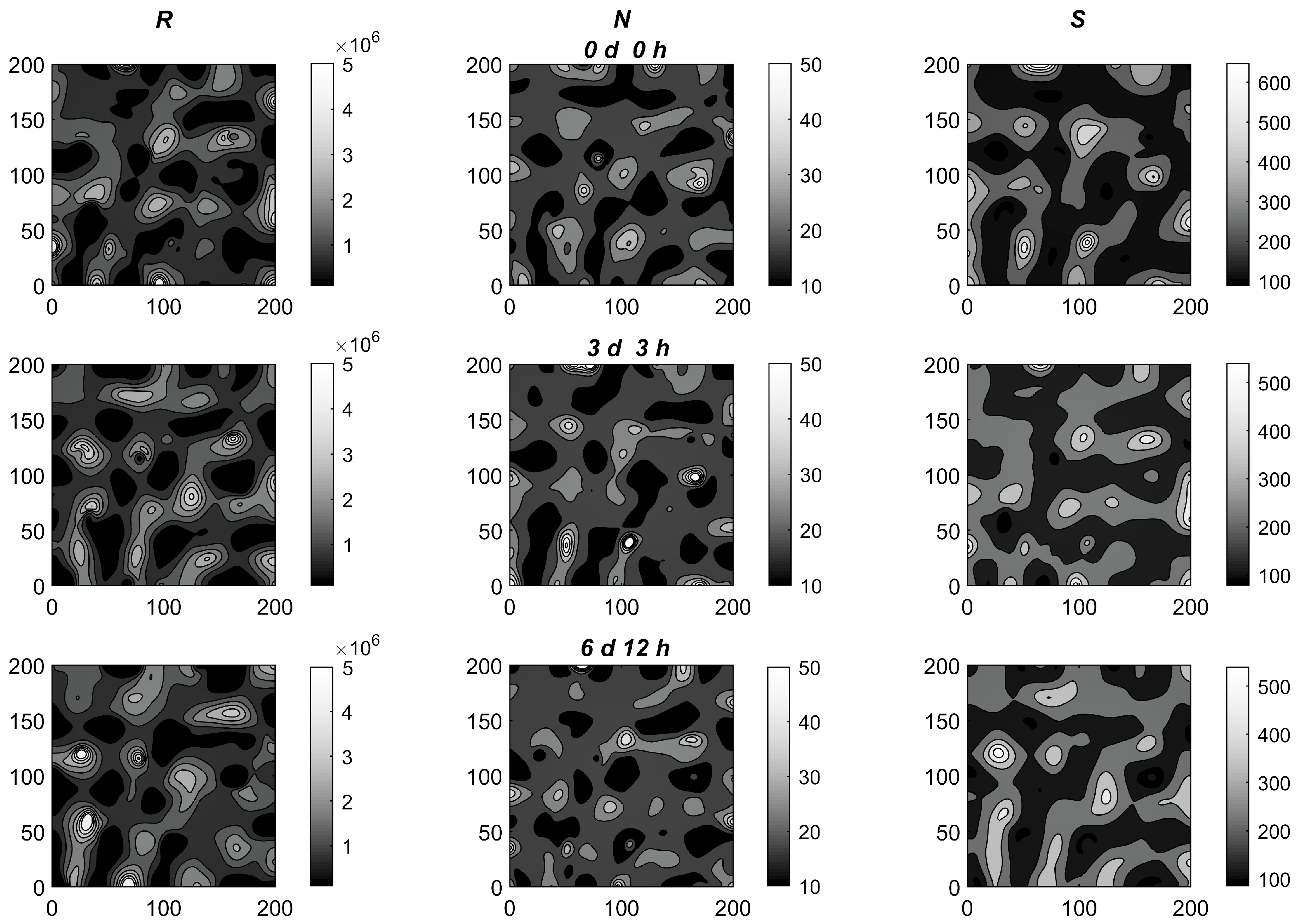
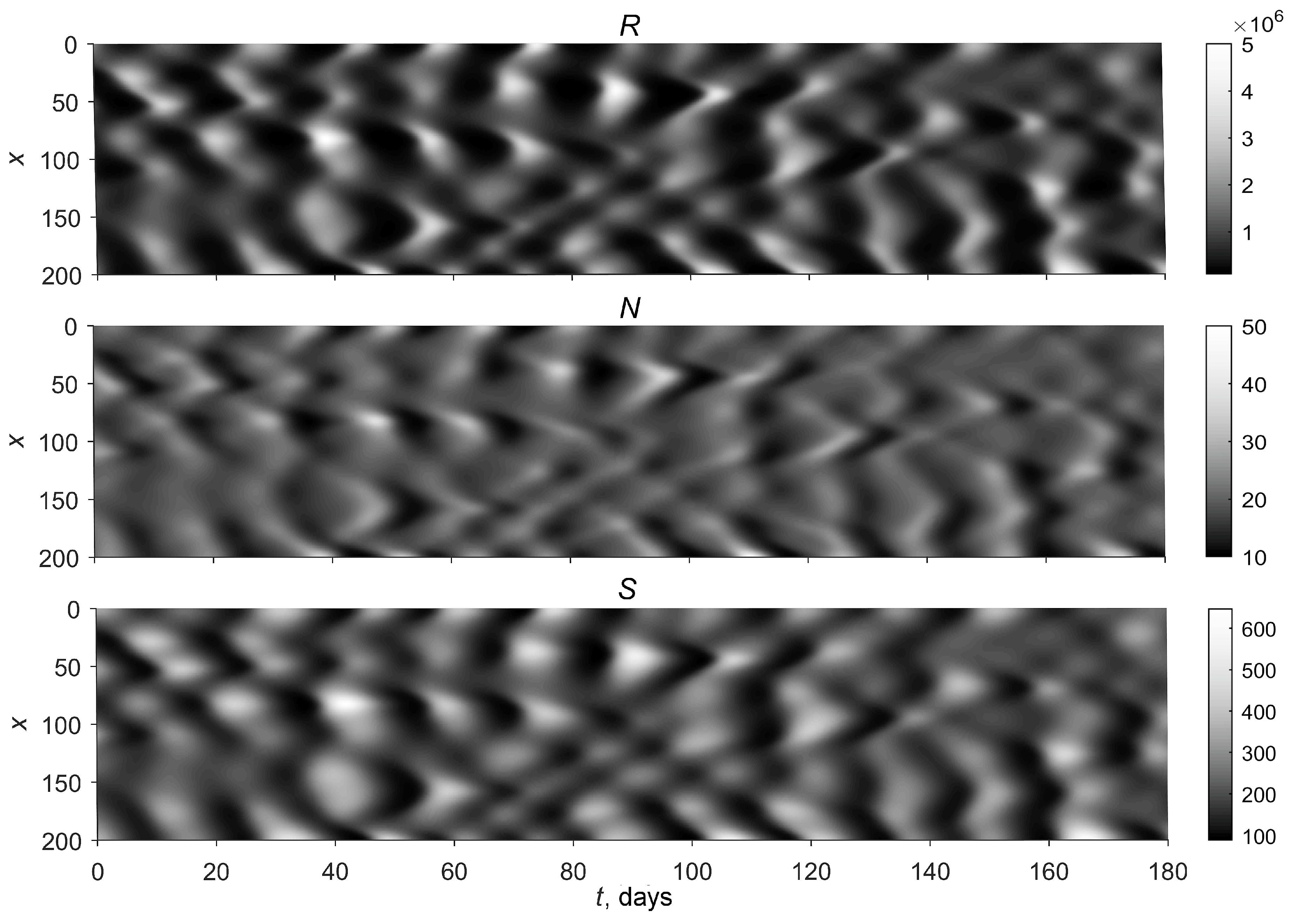
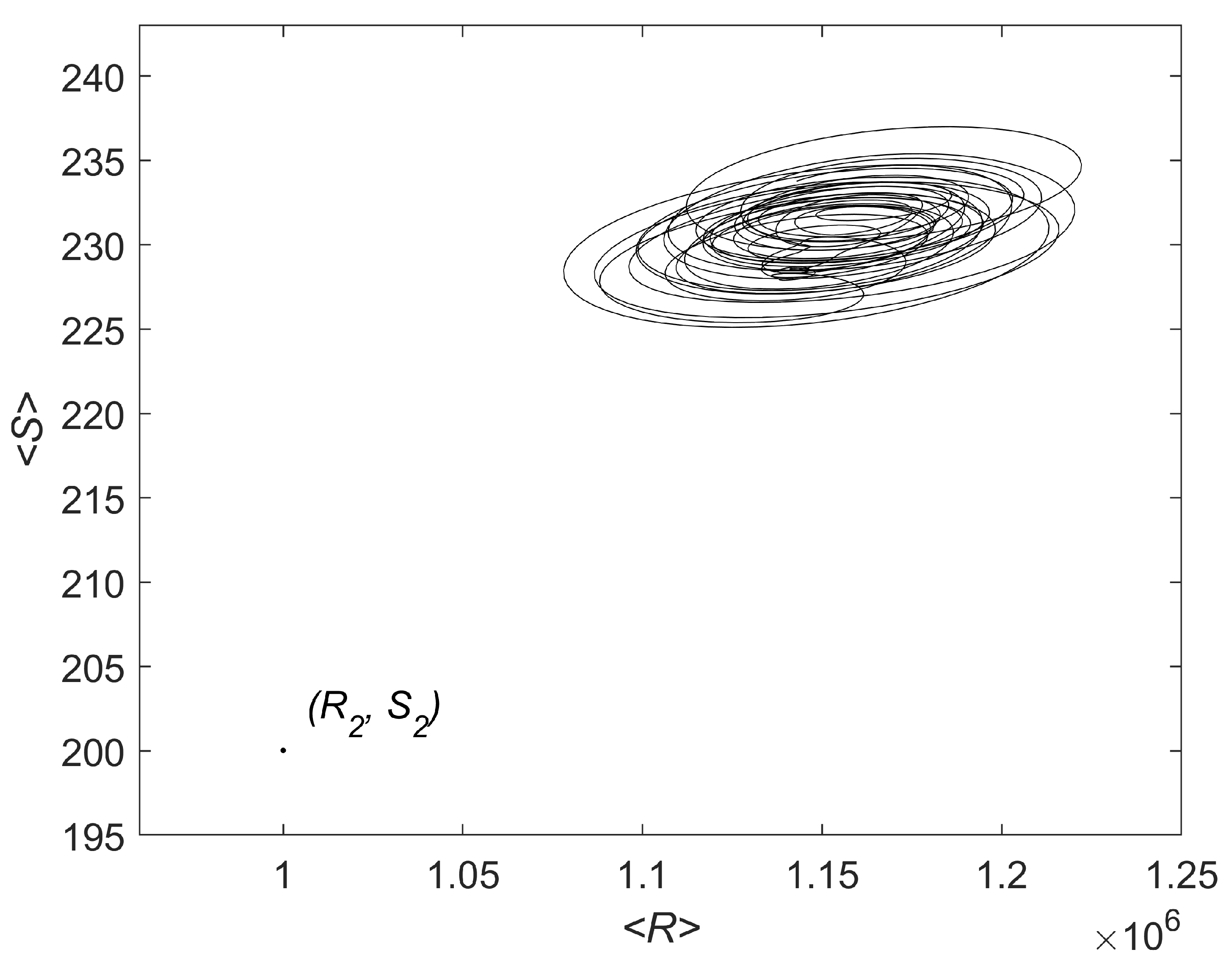
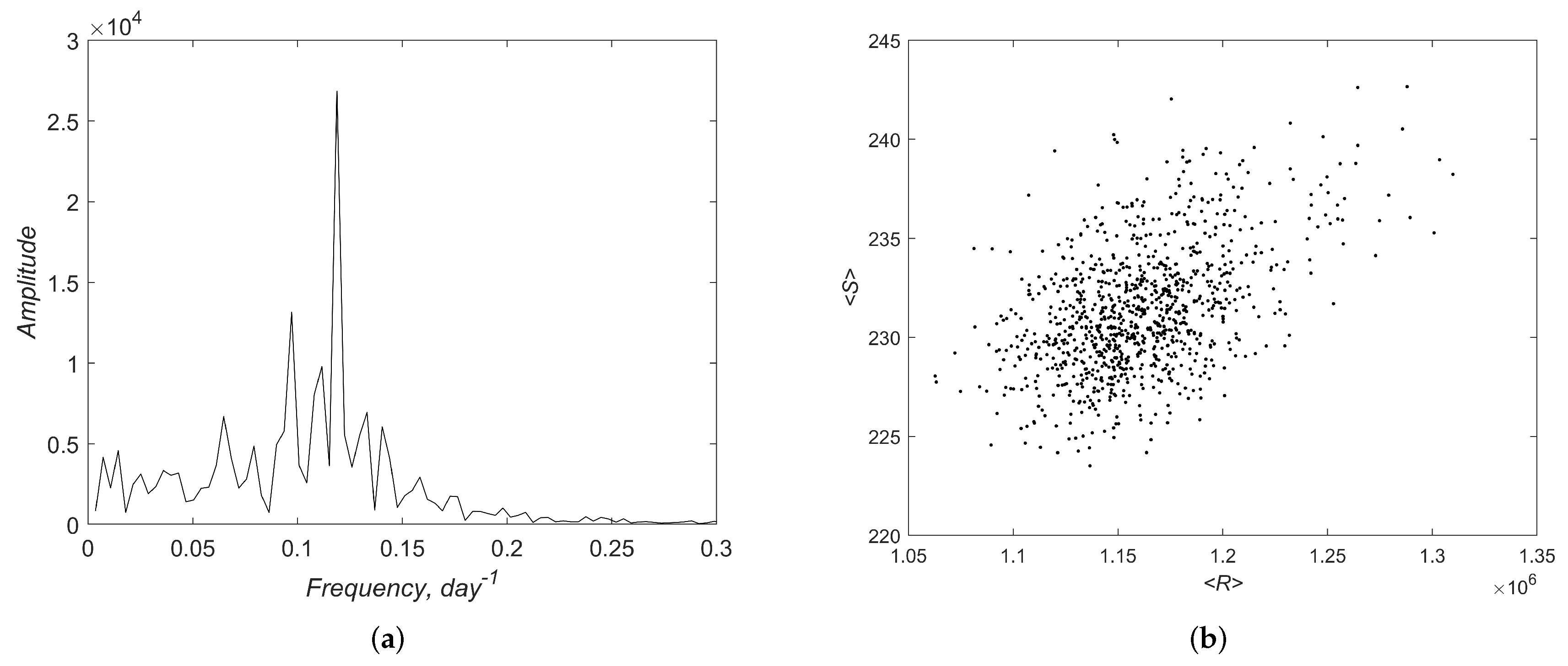
For numerical integration of the dimensionless continuous model (7)–(11) over the rectangular habitat domain $\mathsf{\Omega }=\left[0,1\right]\times \left[0,L\right]$ the following scheme was applied. We use a regular spatial grid $\{\left(x_i,y_j\right)=\left(i{h}_x,j{h}_y,i=0,\cdots ,M_x,j=0,\cdots ,M_y\right)\}$ with step $h_x=1/M_x$ on axis X and step $h_x=1/M_y$ on axis Y. Let $R_{i,j}\left(t\right)=R\left(x_i,y_j,t\right)$, $N_{i,j}\left(t\right)=N\left(x_i,y_j,t\right)$ and $S_{i,j}\left(t\right)=S\left(x_i,y_j,t\right)$ denote respectively the densities of prey (microalgae), predator (harpactiod) and stomach satiety of harpacticoid in each node of the spatial grid. The approximation of system (7)–(9) in internal nodes of the grid $\left(i=1,\cdots ,M_x-1,j=1,\cdots ,M_y-1\right)$ is the following system of ODEs:

$$\begin{array}{c}\hfill \begin{array}{cc}\hfill \frac{d{R}_{i,j}}{dt}& =R_{i,j}\left(1-R_{i,j}-N_{i,j}\right)+\hfill \\ \hfill & +{\delta }_R\left(\frac{R_{i+1,j}-2R_{i,j}+R_{i-1,j}}{h_x^2}+\frac{R_{i,j+1}-2R_{i,j}+R_{i,j-1}}{h_y^2}\right);\hfill \end{array}\end{array}$$

(17)

$$\begin{array}{c}\hfill \begin{array}{cc}\hfill \frac{d{N}_{i,j}}{dt}& =-\frac{1}{h_x}\left(a_{i+1,j}^x\frac{S_{i+1,j}-S_{i,j}}{h_x}+a_{i,j}^x\frac{S_{i,j}-S_{i-1,j}}{h_x}\right)+\hfill \\ \hfill & +\frac{1}{h_x}\left(b_{i+1,j}^x\frac{N_{i+1,j}-N_{i,j}}{h_x}+b_{i,j}^x\frac{N_{i,j}-N_{i-1,j}}{h_x}\right)-\hfill \\ \hfill & -\frac{1}{h_y}\left(a_{i,j+1}^y\frac{S_{i,j+1}-S_{i,j}}{h_y}+a_{i,j}^y\frac{S_{i,j}-S_{i,j-1}}{h_y}\right)+\hfill \\ \hfill & +\frac{1}{h_y}\left(b_{i,j+1}^y\frac{N_{i,j+1}-N_{i,j}}{h_y}+b_{i,j}^y\frac{N_{i,j}-N_{i,j-1}}{h_y}\right);\hfill \end{array}\end{array}$$

(18)

$$\begin{array}{c}\hfill \begin{array}{cc}\hfill \frac{d{S}_{i,j}}{dt}& =R_{i,j}-\eta S_{i,j},\hfill \end{array}\end{array}$$

(19)

where coefficients $a_{i.j}^x$, $a_{i.j}^y$ and $b_{i.j}^x$, $b_{i.j}^y$ take the following values:

$$\begin{array}{c}\hfill \begin{array}{c}\hfill a_{i,j}^x=\left\{\begin{array}{cc}\chi \left(S_{i-1,j}\right)N_{i-1,j},\hfill & S_{i-1,j}<S_{i,j},\hfill \\ \chi \left(S_{i,j}\right)N_{i,j},\hfill & S_{i-1,j}⩾S_{i,j};\hfill \end{array}\right.\end{array}\end{array}$$

(20)

$$\begin{array}{c}\hfill \begin{array}{c}\hfill a_{i,j}^y=\left\{\begin{array}{cc}\chi \left(S_{i,j-1}\right)N_{i,j-1},\hfill & S_{i,j-1}<S_{i,j},\hfill \\ \chi \left(S_{i,j}\right)N_{i,j},\hfill & S_{i,j-1}⩾S_{i,j};\hfill \end{array}\right.\end{array}\end{array}$$

(21)

and

$$\begin{array}{c}\hfill \begin{array}{c}\hfill b_{i,j}^x=\left\{\begin{array}{cc}\mu \left(S_{i-1,j}\right),\hfill & N_{i-1,j}<N_{i,j},\hfill \\ \mu \left(S_{i,j}\right),\hfill & N_{i-1,j}⩾N_{i,j};\hfill \end{array}\right.\end{array}\end{array}$$

(22)

$$\begin{array}{c}\hfill \begin{array}{c}\hfill b_{i,j}^y=\left\{\begin{array}{cc}\mu \left(S_{i,j-1}\right),\hfill & N_{i,j-1}<N_{i,j},\hfill \\ \mu \left(S_{i,j}\right),\hfill & N_{i,j-1}⩾N_{i,j}.\hfill \end{array}\right.\end{array}\end{array}$$

(23)

On the boundaries, system (7)–(11) was approximated with the central differences, introducing dummy nodes and taking into account boundary conditions (10).

Approximation (17)–(23) is an upstream finite difference scheme built according to standard approaches [17,18]. As proved in [19], (i) this scheme saves the conservancy property of the initial continuous model (7)–(11) (i.e., the total abundance of predators in the system is kept constant); (ii) the equilibria (12) are also equilibria of (17)–(23); (iii) the stability condition analytically obtained in [11] for the non-trivial stationary homogeneous regime of model (7)–(11) holds true with high accuracy for the discretized model (17)–(23). Paper [19] presents examples of spatially-heterogeneous dynamic regimes obtained by simulation with the discretized approximation to the dimensionless model (7)–(11) for small supercritical values of bifurcation parameters and various sizes of spatial domain $\mathsf{\Omega }$.

Spatial grid built with $M_x$ and $M_y$ regular nodes along X and Y axes respectively, results in a high-dimensional system of $3\times M_x\times M_y$ ordinary differential equations (ODEs), which is then integrated by the Runge –- Kutta method of the fifth order RKF45 improved by Richardson, with precision control and automatic time-step selection [20]. The minimum number of nodes taken in the simulations was $M_x=M_y=100$, producing a system of $3\times 100\times 100=30,000$ ODEs. The accuracy of spatial discretization was checked on doubled grid. The integration method is realized in C++ on a High-Performance Computing Cluster “Blokhin”; visualization of solutions was obtained with the MATLAB development environment.

3.2. Simulations

In order to compare simulated pattern with these akin to observed in nature, we shall first choose realistic values of the model parameters. We do this basing on the following knowledge about the modelled species.

The diatom microalgae cells replicate 1–3 times per day, thus $r\in \left[0.0006,0.0015\right]$. The average amount of the diatoms is $0.1–5\times {10}^6$ cells per ${\mathrm{cm}}^2$, i.e., $\langle R\rangle \stackrel{\mathrm{def}}{=}\frac{1}{\left|\mathsf{\Omega }\right|}{\int }_{\mathsf{\Omega }}Rd\mathbf{x}\in \left[0.1,5\right]\times {10}^6$. The maximum possible density of microalgae can be 5–10 times higher than the average level, i.e., $K\in \left[2.5,50\right]\times {10}^6$. The average harpacticoid density is 20–50 ind. per ${\mathrm{cm}}^2$, thus $\langle N\rangle \stackrel{\mathrm{def}}{=}\frac{1}{\left|\mathsf{\Omega }\right|}{\int }_{\mathsf{\Omega }}Nd\mathbf{x}\in \left[20,50\right]$. The average number of algal cells per a copepod gut is 150–800 cells, i.e., $\langle S\rangle \stackrel{\mathrm{def}}{=}\frac{1}{\left|\mathsf{\Omega }\right|}{\int }_{\mathsf{\Omega }}Sd\mathbf{x}\in \left[150,800\right]$. The maximum ration of the harpacticoid copepod come to 10–15 cells per minute, i.e., $max\left(ϵaR\right)⩽15$. The mean squared length of individual copepod replacement $\overline{l^2}$ is estimated as 25 $\mathrm{c}{\mathrm{m}}^2$ per minute with temporal resolution of the model $\tau$ equal to 1 min. The size of a typical patch of harpacticoid aggregation varies from 0.5–1 $\mathrm{c}{\mathrm{m}}^2$ to several square meters, though patches of several square decimeters in size are prevailing. The expected lifetime of a patch is estimated as several days.

The above-mentioned observations help choosing feasible values of the other parameters based on simulation outcomes. In particular, coefficients of the frequency function (15) were assign as $k_1=0.0066$ and $k_2=1.4057\times {10}^{-4}$. Taking into account the ranges of variables and expressions for the non-trivial stationary homogeneous regime $\left(R_2,N_2,S_2\right)$ in (12), one gets additional restrictions for the model calibration:

$$\begin{array}{c}\hfill K\left(1-\frac{a\langle N\rangle }{r}\right)\in \left[0.1,5\times {10}^6\right]\mathrm{and}\frac{ϵaK}{\eta }\left(1-\frac{a\langle N\rangle }{r}\right)\in \left[150,800\right].\end{array}$$

Figure 1 and Figure 2 represent stabilized numerical solution of model (1)–(4), (16) for spatial domain $\mathsf{\Omega }=\left[0,200\mathrm{cm}\right]\times \left[0,200\mathrm{cm}\right]$ obtained with parameters presented in

Table 4. Values of the model parameters used in simulations.

Parameter	Dimensional Model (1)–(4), (16)	Dimensionless Model (7)–(10), (16)
r	0.001	1
$L_x$	200	1
$L_y$	200	1
K	$1\times {10}^7$	1
a	$4.5\times {10}^{-5}$	1
$ϵ$	$7.4089\times {10}^{-4}$	1
$\eta$	$1.667\times {10}^{-4}$	0.1667
${\delta }_R$	${10}^{-3}$	$2.5\times {10}^{-5}$
$\langle N\rangle$	20	0.9

, where both dimensional and dimensionless parameters converted according to conversion formulas in Table 3 are given.

Initially diatom population was distributed randomly. Namely, for the corresponding dimensionless system (7)–(10), initial conditions (11) are determined by function ${\phi }_R=R_2+0.001·\xi$, where $\xi$ is a random value uniformly distributed over $\left[-1,1\right]$. Initial spatial distribution of the harpacticoid copepod population was taken homogeneous, ${\phi }_N=\langle N\rangle$, with equal amount of the available food at each spatial position, i.e., ${\phi }_S=S_2$. Here $R_2$ and $S_2$ are the values of the dimensionless variables at homogeneous stationary solution (12). The discrete approximation of the model (17)–(23) was built with regular spatial grid with $M_x=M_y=150$ (system of $67,000$ ODEs).

The simulated pattern represents dynamic mosaics of patches arising and disappearing in a few days. Temporally emerging aggregations of the harpacticoid copepods move towards areas of higher values of the trophotaxis stimulus S, locally depleting the microalgae population. The shapes and sizes of simulated patches of the copepods vary widely in time and in space from small temporal formations of a few square centimeters to large aggregations covering several square decimeters. The average density of copepods in the simulated aggregations exceeds 30 individuals per square centimeter. The spatial pattern evolves rapidly in time, changing radically and unpredictably. Basing on observations on the microalgae population distribution in Figure 1, only a rough guess can be made regarding spatial location of aggregations of copepod in the future. Spatiotemporal plot in Figure 2, presenting dynamics of the model variables at section $y=50\mathrm{cm}$ of the considered domain $\mathsf{\Omega }=\left[0,200\mathrm{cm}\right]\times \left[0,200\mathrm{cm}\right]$, helps revealing that patch of harpacticoid density emerges during period varying from 3 to 7 days after formation of a patch of diatom microalgae. However, a short increase of algal density does not immediately cause forming the copepod patch in that location. The changes in distribution of the trophotaxis stimulus S start before the changes in spatial pattern of the consumer density N. To be effectively attractive for the migrating consumer, favorable conditions should last during some period specific for the harpacticoid copepods.

Figure 3 presents projection of the model trajectory onto the plane $\left(\langle R\rangle ,\langle S\rangle \right)$ of the above-defined spatially averaged density of microalgae and individual satiety of harpacticoid. The trajectory demonstrates chaotic oscillations that correspond to stabilized dynamics of the model.

Noteworthily, point $\left(R_2,S_2\right)$ representing in Figure 3 spatially homogeneous solution $\left(R_2,N_2,S_2\right)=\left({10}^6,20,200\right)$, is situated noticeably to the left and below of the domain occupied by the migration-model trajectory. In other words, this stationary homogeneous state which is stable without prey–taxis, corresponds to the situation of overgrazing (permanently low abundance of prey tightly controlled by permanently hungry predator). Due to their spatial feeding behavior, harpacticoid copepods increase both individual consumption and density of microalgae population, by maintaining spatially-heterogeneous dynamics of the ecosystem. We have also computed the Fourier transform of the average prey density $\langle R\rangle$ and built the projection onto the phase plane $\left(\langle R\rangle ,\langle S\rangle \right)$ of the Poincaré section defined by the hyperplane $N\left(50,50,t\right)=\langle N\rangle$. The results of these computations shown in Figure 4 provide additional evidences of complexity of the simulated dynamics. In particular, Figure 4a shows a broad banded amplitude spectrum over a large frequency span what is a typical indication of chaos (compare this spectrum with plot obtained for clearly periodic dynamics in Figure A3). The cloud-like Poincaré map in Figure 4b, which does not consist of either a finite set of points or a closed orbit, presents another sign of chaotic behaviour of the model (see, e.g., [21]). Additionally, the Fourier analysis reveals presence of a periodic component in simulated oscillation; there is a peak amplitude at frequency 0.1188 $\mathrm{d}\mathrm{a}{\mathrm{y}}^{-1}$ which corresponds to dominating period of 8.42 days.

4. Discussion and Conclusions

System (1)–(6) describes a spatial prey–predator model with slowly diffusive (almost immobile, as compared with predator) prey (microalgae) and actively-mobile predator (copepods). In the model presented here (hereinafter referred to as TZA model), predator’s migrations are explicitly formalized as indirect (or equivalently, inertial) prey–taxis stimulated by the degree of starvation, which leads to the Patlak–Keller–Segel flux of the predator population density [8,11]. As shown in [22,23,24,25,26,27,28,29], in the frameworks of the taxis–diffusion–reaction systems this approach enables us to account for the inertial delay in the consumer’s response to varying distribution of the prey. Recently, another model of the same biological system has been presented in [7] (hereinafter referred to as SA model). The main differences of these two models are following:

• The TZA model is continuous in both space and time, while the cellular automata-based SA model is spatially discrete;
• Migration process is continuous in TZA but periodic (semidiurnal) in SA model, imitating the tidal rhythm;
• in TZA, the environment is spatially homogenous, while both cases (homogeneous and heterogeneous environment for prey) are considered in SA model;
• In both models, the predator migrations are simulated as random walk; the distances of movement are unrestricted (normally distributed) in TZA, while restricted (either equiprobably distributed in a fixed neighborhood of a starting point or partly directed by a taxis) in SA model;
• Functional response of predator is the Lotka–Voltera (linear) in TZA but the Holling type III (sigmoid) in SA model;
• The relationship between the frequency of predator migrations and their degree of starvation (stimulus-response function) is described by inverse parabolic function (15) in TZA but by S-shaped function in SA model.

Despite these differences in approaches applied, the two models yield principally similar results, both producing complex spatiotemporal dynamics of the studied biological system. In simulations under biologically realistic values of parameters, both models demonstrate plausible features of the modelled distribution of prey and predator populations. In particular, the spatial scale of patchiness (i.e., characteristic sizes of patches) is similar in both models and corresponds to that observed in nature. This spatial pattern changes more slowly in SA model, because of the semidiurnal periodicity of migrations, in contrast to continuous migrations assumed in TZA model. Thus, both models rather adequately reproduce the micro-scale spatial pattern observed in natural populations of diatom microalgae and harpacticoid copepods. It is significant to note that such chaotic behavior is intrinsic property of the system and emerges in both models without any additional assumptions, such as environmental heterogeneity, barriers for dispersal, non-local interactions or external disturbing forces.

The simple mechanism implied, namely, the increasing migration frequency as local response of individual predator on its starvation, is sufficient to generate the complex spatiotemporal behavior. Moreover, both SA and TZA models show that spatially-heterogeneous regimes appearing with starvation-dependent migrations, as compared with stationary homogeneous regime without prey–taxis, provide the significant advantage for both predator (increasing its food consumption rate) and prey (increasing its average abundance). Thus, this implied mechanism is evolutionary advantageous strategy, which allows prey and predator to coexist safely and avoid the collapse of total overgrazing, and therefore increases the efficiency of the whole system. The effect of increased viability of trophic system due to the active predator’s movements was earlier revealed for spatial prey–predator models with the indirect (inertial) prey–taxis [22,23,27,30].

The proposed model of indirect prey–taxis (1)–(6), (15) qualitatively reproduces micro-scale spatial pattern observed in natural diatom-harpacticoid trophic system. In particular, the model with parameters fitted on the basis of field observations and current knowledge about ecology of the studied species, enables the simulation of spatiotemporal chaotic dynamics with plausible characteristic size and expected lifetime of the copepod density patches.

The cause of spatial heterogeneities in the model is the behavioral response of harpacticoid copepods (predators) on distribution of diatom microalgae (prey). Migration activity of individual harpacticoid depends on its satiety. Food-replete harpacticoides prefer to stay in their feeding areas, very rarely coming out of the bottom sediment. The frequency of individual relocation-jumps increases with starvation, causing the repeated horizontal migrations of a hungry copepod within the water column, what gives the consumer a chance to reach a more suitable location. As shown in [11], such individual behavior of copepods leads to prey–taxis observed at the level of population. The prey–taxis term is explicitly included into the balance equation of predator population density of system (1)–(3). Dense aggregations of harpacticoids and at the same time, temporal refuges for diatoms in locations where copepods are virtually absent emerge in the system due to prey–taxis movements. This complex dynamics helps harpacticoids to overcome shortage of food by increasing both individual consumption and total abundance of the diatom population.

In conclusion, we shall emphasize that the predator’s Equation (2) includes no terms for birth and death of the harpacticoid populations because these demographic processes are much slower than growth of the microalgal population and than spatial spread of the species densities. Under this assumption, stationary homogeneous state $\left(R_2,N_2,S_2\right)$ of model (1)–(6) remains stable in the absence of prey–taxis term in (2) (see also [8]). Thus, the model (1)–(6) can be viewed as the minimal model capable of explaining and reproducing qualitatively realistic spatiotemporal dynamics of the microalgae–harpacticoid system, which emerges solely due to spatial behavior of harpacticoid copepods. Accounting for indirect prey–taxis in prey–predator models allows us to study such feeding behaviour as an evolutionary advantageous strategy of migrating consumers.

References

1. Azovsky, A.I.; Chertoprud, E.S. Spatio-temporal dynamics of the White Sea littoral Harpacticoid community. Oceanology 2003, 43, 103–111. [Google Scholar] [CrossRef]
2. Fleecer, J.W.; Palmer, M.A.; Moser, E.B. On the scale of aggregation of meio-bentic copepodes on a tidal mudflat. Mar. Ecol. 1990, 11, 227–237. [Google Scholar] [CrossRef]
3. Azovsky, A.; Chertoprood, E.; Saburova, M.; Polikarpov, G. Selective feeding of littoral harpacticoids on diatom algae: Hungry gourmands? Mar. Biol. 2005, 148, 327–337. [Google Scholar] [CrossRef]
4. Sach, G.; Bernem, H. Spatial patterns of Harpacticoida copepods on tidal flats. Senchenberg. Mar. 1996, 26, 97–106. [Google Scholar]
5. Sun, B.; Fleeger, J.W. Spatial and temporal patterns of dispersion in meiobenthic copepods. Mar. Ecol. Prog. Ser. 1991, 71, 1–11. [Google Scholar] [CrossRef]
6. Woods, D.R.; Tietjen, J.H. Horizontal and vertical distribution of meiofauna in the Venezuela Basin. Mar. Geol. 1985, 68, 233–241. [Google Scholar] [CrossRef]
7. Smirnova, E.A.; Azovsky, A.I. Modelling of spatially distributed predator-prey system with periodically migrating predator (Case study of the White Sea inertidal harpacticoids and benthic microalgae). Oceanology 2020, 60, 89–97. [Google Scholar] [CrossRef]
8. Tyutyunov, Y.V.; Zagrebneva, A.D.; Surkov, F.A.; Azovsky, A.I. Microscale patchiness of the distribution of copepods (Harpacticoida) as a result of trophotaxis. Biophysics 2009, 54, 355–360. [Google Scholar] [CrossRef]
9. Keller, E.F.; Segel, L.A. Model for Chemotaxis. J. Theor. Biol. 1971, 30, 225–234. [Google Scholar] [CrossRef]
10. Patlak, C.S. Random walk with persistence and external bias. Bull. Math. Biophys. 1953, 15, 311–338. [Google Scholar] [CrossRef]
11. Tyutyunov, Y.V.; Zagrebneva, A.D.; Surkov, F.A.; Azovsky, A.I. Derivation of density flux equation for intermittently migrating population. Oceanology 2010, 50, 67–76. [Google Scholar] [CrossRef]
12. Painter, K.J. Mathematical models for chemotaxis and their applications in self-organisation phenomena. J. Theor. Biol. 2019, 481, 162–182. [Google Scholar] [CrossRef] [PubMed] [Green Version]
13. Jeschke, J.M.; Kopp, M.; Tollrian, R. Consumer-food systems: Why type I functional responses are exclusive to filter feeders. Biol. Rev. 2004, 79, 337–349. [Google Scholar] [CrossRef] [PubMed]
14. De Troch, M.; Grego, M.; Chepurnov, V.A.; Vincx, M. Food patch size, food concentration and grazing efficiency of the harpacticoid Paramphiascella fulvofasciata (Crustacea, Copepoda). J. Exp. Mar. Biol. Ecol. 2007, 343, 210–216. [Google Scholar] [CrossRef]
15. Leising, A.W.; Franks, P.J. Does Acartia clausi use an area-restricted search foraging strategy to find food. Hydrobiologia 2002, 480, 193–207. [Google Scholar] [CrossRef]
16. Kern, J.C. Active and passive aspects of meiobenthic copepod dispersal at two sites near Mustang Island, Texas. Mar. Ecol. Prog. Ser. 1990, 60, 211–223. [Google Scholar] [CrossRef]
17. Morton, K.W.; Mayers, D.F. Numerical Solution of Partial Differential Equations; Cambridge University Press: Cambridge, UK, 1994; 227p. [Google Scholar] [CrossRef]
18. Samarsky, A.; Gulin, A. Numerical Methods; Publishing House Nauka: Moscow, Russia, 1989; 430p. (In Russian) [Google Scholar]
19. Zagrebneva, A.; Tyutyunov, Y.; Surkov, F.; Azovsky, A. Numerical realization of taxis-reaction-diffusion model describing population dynamics in predator-prey system. IZvestiya Vuzov. Sev. Kavk. Reg. Nat. Sci. Ser. 2010, 2, 12–16. (In Russian) [Google Scholar]
20. Kahaner, D.; Moler, C.; Nash, S. Numerical Methods and Software; Prentice-Hall Inc.: Upper Saddle River, NJ, USA, 1989; 495p. [Google Scholar]
21. Moon, F. Chaotic and Fractal Dynamics: Introduction for Applied Scientists and Engineers; Wiley-VCH: Weinheim, Germany, 1992; 508p. [Google Scholar]
22. Arditi, R.; Tyutyunov, Y.; Morgulis, A.; Govorukhin, V.; Senina, I. Directed movement of predators and the emergence of density-dependence in predator–prey models. Theor. Popul. Biol. 2001, 59, 207–221. [Google Scholar] [CrossRef] [Green Version]
23. Govorukhin, V.; Morgulis, A.; Tyutyunov, Y. Slow taxis in a predator–prey model. Dokl. Math. 2000, 61, 420–422. [Google Scholar]
24. Morgulis, A.; Ilin, K. A remark on the disorienting of species due to the fluctuating environment. arXiv 2019, arXiv:1808.02091v4. [Google Scholar]
25. Rai, V.; Upadhyay, R.K.; Thakur, N.K. Complex population dynamics in heterogeneous environments: Effects of random and directed animal movements. Int. J. Nonlin. Sci. Num. 2012, 13, 299–309. [Google Scholar] [CrossRef]
26. Tello, J.I.; Wrzosek, D. Predator–prey model with diffusion and indirect prey-taxis. Math. Mod. Meth. Appl. Sci. 2016, 26, 2129–2162. [Google Scholar] [CrossRef]
27. Tyutyunov, Y.; Sen, D.; Titova, L.I.; Banerjee, M. Predator overcomes the Allee effect due to indirect prey–taxis. Ecol. Complex. 2019, 39, 100772. [Google Scholar] [CrossRef]
28. Tyutyunov, Y.; Titova, L.; Senina, I. Prey–taxis destabilizes homogeneous stationary state in spatial Gause–Kolmogorov-type model for predator–prey system. Ecol. Complex. 2017, 31, 170–180. [Google Scholar] [CrossRef]
29. Tyutyunov, Y.; Zagrebneva, A.D.; Govorukhin, V.N.; Titova, L.I. Numerical Study of Bifurcations Occurring at Fast Time-scale in a Predator–prey Model with Inertial Prey–taxis. In Advance Mathematical Method in Biosciences and Applications; Berezovskaya, F., Toni, B., Eds.; STEAM-H Science, Technology, Engineering, Agriculture, Mathematics & Health; Springer: Cham, Switzerland, 2019; pp. 221–239. [Google Scholar] [CrossRef]
30. Sapoukhina, N.; Tyutyunov, Y.; Arditi, R. The role of prey taxis in biological control: A spatial theoretical model. Am. Nat. 2003, 162, 61–76. [Google Scholar] [CrossRef] [PubMed] [Green Version]
Figure 1. Snapshots of spatial distributions of diatom microalgae R cells · c m 2 , harpacticoid copepods N ind · c m 2 , and satiety of individual harpacticoid S algal   cells · i n d 1 · c m 2 at the indicated moments of time, computed with model (1)–(6) for domain Ω = 200 cm × 200 cm .
Mathematics 08 01065 g001
Figure 2. Spatiotemporal dynamics of variables R, N, S at section y = 50 cm of domain Ω .
Mathematics 08 01065 g002
Figure 3. Phase trajectory of model (1)–(6), (15) in the plane of spatially averaged values R , S . Parameters are given in Table 4. Point R 2 , S 2 depicts the unstable stationary homogeneous state.
Mathematics 08 01065 g003
Figure 4. (a) The Fourier spectrum of the average prey density R . (b) Projection onto the phase plane R , S of the Poincaré map defined by the hyperplane N 50 , 50 , t = N .
Mathematics 08 01065 g004