

Abstract
Sea-level rise magnifies flood hazards, raising the question when adaptation measures need to be taken. Here, we quantify when the recurrence of extreme water level events will double due to projected sea-level rise. Reproducing the most common method based on extreme water levels observed with tide gauges, at least one third of the coastal locations are to expect a doubling of extremes within a decade. However, tide gauges are commonly placed in wave-sheltered harbours where the contribution of waves to water levels is much smaller than at nearby wave-exposed coastlines such as beaches and dikes. In this study, we quantify doubling times at a variety of idealised shorelines based on modelled tides, storm surges and waves. We apply an extreme value analysis that accounts for the joint probability of extreme storm surges and extreme waves. Our results indicate that doubling times at wave-exposed shorelines are longer than those in wave-sheltered harbours, allowing for more time to adapt to magnified flood hazards. The median doubling times of average water levels including parameterised wave set-up are 1.2 to 5 times longer than those of still water levels as observed with tide gauges. For instantaneous water levels including wave run-up, doubling times are an additional 30% to 100% longer. We conclude that tide gauge-based analyses underestimate adaptation times by underestimating the contribution of waves to extreme water levels, and provide a quantitative framework to guide adaptation policy at wave-exposed shorelines.
Export citation and abstract BibTeX RIS

Original content from this work may be used under the terms of the Creative Commons Attribution 4.0 license. Any further distribution of this work must maintain attribution to the author(s) and the title of the work, journal citation and DOI.
1. Introduction
As land-based ice melts and oceans warm, the global mean sea level is projected to rise throughout the 21st century and beyond (Church et al 2013). This rise will impact flood hazards through its effect on extreme water level events (Hunter 2012, Tebaldi et al 2012, Oppenheimer et al 2019) (figure 1(a)). Such events, sometimes referred to as extreme sea levels or extreme coastal water levels (Gregory et al 2019), become more frequent as mean sea level rises. A crucial piece of information in the design of adaptation planning is the time scale at which coastal adaptation measures must be taken (Haasnoot et al 2013, Hinkel et al 2019). In other words: at what rate will flood hazards magnify? One way to quantify this is in terms of the so-called amplification, which is the increase in the average recurrence rate of extreme events (figure 1(a) and (b). The common practice to estimate this amplification is based on historical extreme events observed by tide gauges (e.g. Slangen et al 2017, Rasmussen et al 2018, Frederikse et al 2020). In their Special Report on the Oceans and Cryosphere in a Changing Climate (SROCC), the Intergovernmental Panel on Climate Change (IPCC) used such a tide gauge-based analysis to conclude that historical centennial events will recur at least annually at most coastal locations before the end of the 21st century (IPCC 2019). However, tide gauges are often located in wave-sheltered harbours and measure so-called Still Water Levels (SWLs) which are known to underestimate or fully exclude waves (Melet et al 2018, Woodworth et al 2019, Dodet et al 2019). This raises the question to what extent tide gauge-based estimates of the amplification of extreme water levels are representative for wave-exposed shorelines nearby those tide gauges.
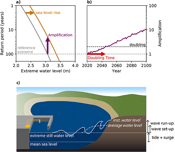
Figure 1. Schematic overview of concepts. (a) The relation between extreme water levels and associated return periods. Arrows illustrate the effect of sea-level rise. (b) Amplification of the historical 1-in-100 year event and an indication of the doubling time. (c) Definitions of water levels. Still Water Levels (SWLs) are those measured by tide gauges, typically within wave-sheltered harbours. Average Water Levels (AWLs) are water levels at the coast including wave set-up. Instantaneous Water Levels (IWLs) include wave run-up.
Download figure:
Standard image High-resolution imageWaves contribute to water levels in two ways (Stockdon et al 2006)(figure 1(c)). First, the breaking of shoreward travelling waves elevates the time-average coastal water level. This process is called wave set-up and contributes to the Average Water Level (AWL), sometimes referred to as mean total water levels (O'Grady et al 2019). Second, individual waves add a periodic oscillation to the water level. Combined with wave set-up, the height of the highest individual waves is called wave run-up and contributes to the Instantaneous Water Level (IWL), sometimes referred to as the total water level. The term extreme water level is therefore an ambiguous one which may refer to SWL, AWL, or IWL. Which definition is most appropriate for coastal adaptation, depends on the local protection policy: if one is concerned with overflow or overtopping risk, one should base the analysis on extreme AWL or IWL respectively. An analysis based on extreme SWLs, however, may only be applicable to specific wave-sheltered areas such as the harbours in which tide gauges are commonly placed. As an additional complication to quantify the contribution of waves to flood hazards, wave set-up and run-up strongly depend on local shoreline properties including its type (e.g. beaches or dikes), material and steepness.
In this study, we quantify the amplification of extreme AWLs and IWLs at a quasi-global set of coastal locations and compare these to the amplification of extreme SWLs as derived from tide gauge records. Even though previous studies have estimated these amplifications (Vitousek et al 2017, Vousdoukas et al 2018), their treatment of waves is idealised. We build upon these previous works by (1) using an advanced method to reduce biases arising from parameter choices (Wahl et al 2017), (2) accounting for the joint probability of extreme waves and storm surges to optimally extract the information from short time series (Marcos et al 2019), (3) applying our methodology to a wide range of shorelines to increase the applicability at each coastal location, and (4) explicitly contrasting the amplification of extreme AWLs and IWLs to that of extreme SWLs to translate tide gauge-based estimates to policy-relevant information.
2. Methods
As a proxy for the adaptation time to magnified flood hazards, we quantify the doubling time (Vitousek et al 2017) of extreme SWLs, AWLs, and IWLs. Using two different statistical methods, we quantify historical extreme water levels and estimate the height of a reference extreme: the 1-in-100 year event. We combine these historical extreme water levels with a time series of projected mean sea-level rise to quantify the amplification of this reference extreme, which is the decrease in the return period (figure 1(a)). The doubling time is defined as the time until this amplification exceeds the value 2, marking the moment when the 1-in-100 year event has become a 1-in-50 year event (figure 1(b)).
The statistical methods are applied to a quasi-global set of 130 tide gauge locations from the Gesla-2 dataset (Woodworth et al
2016). We have selected this subset of locations randomly, with a minimum distance of 250 kilometres between all locations, to compensate for the overrepresentation of available tide gauge records in the northern hemisphere mid-latitudes (
For the estimation of extreme SWLs, we apply the single variate method, which is the simplest and most widely used type of extreme value analysis and which can be directly applied to tide gauge records. In this study, we adopt the peaks-over-threshold approach which extracts peak water levels from a time series, to which a theoretical distribution, the generalised Pareto distribution, can be fitted. The fit is highly sensitive to the choice of threshold (Wahl et al
2017) which is commonly prescribed or determined using visual techniques (Coles et al
2001). As such a manual method cannot be applied (semi-)automatically to a large number of observational records, we adopt an automatic threshold selection that aims for an optimal balance between the bias and variance in extremes (Northrop et al
2017). The theoretical distribution, schematically represented by the grey line in figure 1(a), is finally extrapolated to estimate the height of the 1-in-100 year event. To quantify the impact of mean sea-level rise on the recurrence frequency of this extreme event, we shift the theoretical distribution horizontally; the associated vertical shift then represents the amplification. Note that this approach does not account for future changes in the distribution of extremes, which we discuss further in section 6. Regional sea-level rise projections are taken from IPCC's SROCC (Oppenheimer et al
2019) and referenced to present-day values. As both the theoretical distribution and the regional sea-level rise projection come with an uncertainty, the amplification is quantified using a Monte Carlo method (
Several issues arise when incorporating wave set-up or run-up in the quasi-global estimation of doubling times of extreme water levels. First, no global continuous measurements exist, so we use modelled waves instead. Second, both wave set-up and run-up depend strongly on local shoreline properties. These are largely undocumented and may vary in time due to natural or human factors, preventing the explicit modelling on a large scale. Hence, we resort to parameterisations of wave set-up and run-up in terms of deep-sea wave properties. Three parameterisations exist which express wave set-up and run-up in terms of significant wave height and mean wave period: one for dissipative beaches (Stockdon et al
2006), one for sandy beaches (Stockdon et al
2006) and one for rock slopes such as dikes (van der Meer and Stam 1992). These latter two parameterisations additionally depend on the slope of the shoreline. As shoreline properties differ at small spatial scales nearby tide gauges, we cannot a priori apply the most appropriate parameterisation to each coastal location. Rather, we compute doubling times of AWLs and IWLs for a range of hypothetical shorelines: sheltered harbours without wave set-up or run-up, dissipative and steep sandy beaches, and gentle and steep rocky dikes (
Several previous studies have quantified extreme AWLs or IWLs using an equivalent single variate method as described above. These extract peaks from a single time series of water levels including tides, storm surges, and parameterised wave set-up or run-up (Melet et al 2018, Vitousek et al 2017). Others have applied this method to flood levels (the sum of storm surge and wave set-up or run-up), separately adding astronomic tides (Vousdoukas et al 2018). However, extreme value analysis is limited by available data and the single variate method does not make optimal use of all information contained in these data (see discussion by Zheng et al 2017). In particular, it does not explicitly account for the dependence between extreme storm surges and waves which has been shown to influence extreme water levels (Marcos et al 2019). To optimally extract and use the information in historical data, a number of studies recommend the use of a joint probability method which explicitly accounts for this co-dependence (Hawkes et al 2002, Callaghan et al 2008, Serafin and Ruggiero 2014).
For this joint probability method, we adopt a dependence model (Heffernan and Tawn 2004). First, we fit a generalized Pareto distribution to the extreme values of three individual variables: modelled storm surge, and reanalysis of deep-sea wave height and mean wave period. Next, we use the dependence model to extract the dependence structure between the extreme values of each set of two variables using a non-linear regression model. From the individual distributions and the dependence structure, a large set (100,000) of artificial extreme events is generated. For each event, AWLs and IWLs are computed by applying the different wave parameterisations and sampling a tidal peak from the empirical distribution of modelled astronomical tides (see
3. Doubling times of Still Water Levels
Using the single variate method, we have computed doubling times for a quasi-global set of 130 coastal locations (Woodworth et al 2016) (figure 2(a)). At least one third of these locations can expect a doubling of extreme SWLs within the coming decade. This number of locations varies slightly between future greenhouse gas emission scenarios: under RCP 2.6, 33% of the locations have a doubling time of less than ten years (figure 2(b)), compared to 41% under RCP 8.5. Locations with longer doubling times are largely distributed over the mid- and high latitudes. A small fraction of these locations should not expect a doubling of extreme SWLs before the end of the 21st century; this fraction depends more strongly on future emissions, ranging from 10% under RCP 2.6 to 3% under RCP 8.5. These locations without a projected doubling in the 21st century are either found at high latitudes (i.e. Scandinavia where post-glacial land uplift counteracts sea-level rise) and in regions where tropical cyclones occur (i.e. the Gulf of Mexico). While regional patterns in mean sea-level rise explain some geographical differences in doubling times, many of these differences are related to location-dependent present-day variability of extremes (Hunter 2012, Vitousek et al 2017, Frederikse et al 2020).

Figure 2. Doubling times of Still Water Levels (SWLs) based on tide gauge observations. (a) Doubling times of the present-day 1-in-100 year event at a quasi-global selection of coastal locations under RCP 4.5. (b) The distribution of doubling times for three emission scenarios. Short doubling times indicate that flood hazards will amplify relatively quickly, implying little time available for adaptation measures.
Download figure:
Standard image High-resolution imageWe define this variability in extremes as the slope of the curve relating the height and return period of extreme water levels (figure 3(a)). This variability in extremes can be interpreted as the difference between rare extremes (i.e. the 1-in-100 year event) and more common ones (i.e. the 1-in-1 year event). We illustrate the influence of this variability on doubling times by contrasting two locations: Hoek van Holland (the Netherlands) and Mossel Bay (South Africa; figure 3(a), dotted lines). At Mossel Bay, the variability in extremes is relatively small. As a consequence, a moderate amount of sea-level rise can induce a substantial amplification of extreme events (figure 3(b)). Hoek van Holland, however, is subject to strong storm surges, which introduce a relatively large variability in extremes. This variability dampens the amplification of extremes, caused by a rise in mean sea level, compared to locations such as Mossel Bay where the variability is limited. The case of Hoek van Holland exemplifies many mid-latitude locations with strong storm surges and relatively long doubling times. This positive relation between the variability in extremes and doubling times may be considered as a general rule for extremes and one may therefore expect that any variability in coastal extremes induced by waves will also impact doubling times.
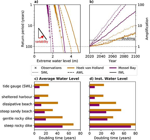
Figure 3. Extreme water levels at two example locations. (a) Present-day return periods based on extreme Still Water Levels, Average Water Levels and Instantaneous Water Levels. Wave set-up and run-up are based for dissipative beaches. The variability in extremes is defined as the slope of each line between the height and return period of extreme water levels (see inset). (b) Associated amplification of the present-day 1-in-100 year event under RCP 4.5. (c) Doubling times of Average Water Levels for under RCP 4.5 for a range of shoreline types. As an indication, the tide gauge-based doubling time of SWLs is included. (d) As panel (c) for Instantaneous Water Levels.
Download figure:
Standard image High-resolution image4. The contribution of waves to doubling times
We illustrate the impact of waves on doubling times for potential dissipative beaches at our two example locations. Both wind waves (dominant at Hoek van Holland) and swell waves (dominant at Mossel Bay) can greatly enhance the variability in extremes with respect to SWLs (figure 3(a)). Not surprisingly, this effect is largest for IWLs including wave run-up (solid lines). Whereas the variability in extremes due to tides and surges is moderate at Mossel Bay, swell waves can dominate the variability in extreme AWLs and IWLs. This enhanced variability slows down the amplification, as shown in figure 3(b) for RCP 4.5, and lengthens the doubling time of the 1-in-100 year event. Even though the variability in extreme SWLs at Hoek van Holland is already substantial, wind waves co-occurring with extreme storm surges further enhance the variability in extreme AWLs and IWLs. We have not found evidence for any discernible difference between the impact of wind waves and swell waves on doubling times. Rather, these results confirm that waves follow the general rule that an enhanced variability in extremes slows down amplification rates and lengthens doubling times.
These results can directly guide coastal adaptation policy. Based on tide gauge records, policy makers should plan their adaptation strategy according to doubling times of 25 and 9 years at Hoek van Holland and Mossel Bay respectively (figure 3(c) and (d)). These estimates agree well with doubling times for sheltered harbours derived from modelled tides and surges (24 and 9 years). However, if policy makers can acquire a qualitative and quantitative description of their shoreline and formulate a clear protection policy, they can revise these numbers. For example, if they are concerned with protecting a stretch of steep sandy beaches against overtopping, these doubling times should be revised to 55 and 29 years respectively. The available time for adaptation at these shorelines is therefore underestimated in the tide gauge-based analysis by a factor of 2 (Hoek van Holland) and 3 (Mossel Bay). We have computed doubling times of AWLs and IWLs using the single variate method as well and find that this method underestimates doubling times (see appendix
5. Greenhouse gas emission scenarios, shoreline properties and coastal hazards
Doubling times from the quasi-global set of locations (figure 4) confirm the conclusions drawn from the two example locations (figure 3). The doubling times of extreme water levels in sheltered harbours, based only on modelled tides and surges, are in close agreement with the doubling times of extreme SWLs (figure 2(b)). This indicates that observations can be interpreted as extreme water levels in absence of wave set-up and run-up, and the model reproduces these extremes well. The doubling times of AWLs and IWLs at dissipative beaches are in overall agreement with previous estimates derived from a single variate method (Vitousek et al
2017). However, we see that without accounting for the joint probability between extreme waves and storm surges, doubling times are underestimated (see appendix

Figure 4. Dependency of doubling times on emission scenarios and shoreline properties for (a) Average Water Levels including wave set-up and (b) Instantaneous Water Levels including wave run-up.
Download figure:
Standard image High-resolution imageFor the doubling on short time scales, e.g. ten years, the influence of greenhouse gas emission scenarios is relatively small (figure 4). As emission scenarios only diverge by mid-century (Church et al 2013), projected mean sea-level rise for the coming decades is largely independent of future emissions. The fraction of locations with doubling times below ten years does, however, strongly depend on shoreline properties and coastal hazards (overtopping or overflow). Whereas the tide gauge-based analysis indicates that at least 33% of the locations may expect a doubling of extremes within ten years, this fraction strongly declines when waves are accounted for, in particular at steeper shorelines. For AWLs at steep sandy beaches, for example, merely 4–7% of the locations can expect such a rapid amplification of extremes. For IWLs, such short doubling times are only expected in sheltered harbours. Whether coastal locations should be concerned about a doubling of extremes within the coming decade therefore primarily depends on local shoreline properties and the coastal hazard of interest, rather than future emissions.
A reduction in future emissions can, however, significantly lengthen already long doubling times. To illustrate this, let us first consider the high-emission scenario RCP 8.5. For AWLs at dissipative beaches, the median doubling time is 17 years. A strong emission reduction to RCP 2.6 would merely extend this median doubling time to 21 years. However, if we consider AWLs at steep dikes, the median doubling time under RCP 8.5 is 47 years. At such shorelines, emission reductions can extend the median doubling time to more than 80 years. In addition, median doubling times of IWLs are 30–100% longer than those of AWLs. These results indicate that waves not only lengthen the doubling times of extremes, providing coastal communities with more time to adapt, but they also demonstrate the benefits of emission reductions. These reduce mean sea-level rise toward the second half of the 21st century, thereby yielding longer doubling times.
6. Discussion
The central aim of this paper was to assess the impact of neglecting waves on the amplification of extreme water levels. We find that waves can lengthen doubling times, placing the usage of tide gauge-based analyses in a more general perspective. In this study, we have exclusively considered the amplification of extremes induced by mean sea-level rise and how this amplification depends on local differences in the variability in present-day extremes. However, we have not considered projected changes in storm surges, tides or waves. Locally, changes in waves (Wang et al 2014, Reguero et al 2019, Serafin et al 2019, Morim et al 2019), or non-linear interactions between mean sea-level and waves (Storlazzi et al 2018), tides (Pickering et al 2017), and surges (Idier et al 2019) may further lengthen or shorten doubling times, though on a global scale, changes in extremes appear to be dominated by mean sea-level rise (Vousdoukas et al 2018). Besides these long-term trends induced by a changing climate, natural variability on seasonal to interannual time scales can further contribute to a temporary acceleration or deceleration of the amplification of extremes.
The doubling time of extreme water levels is an indicator for the time scale at which adaptation measures need to be taken. However, it is a poor indicator for the required extent of these adaptation measures. A better indicator for this extent is the changed height of extreme events with a given return period, which is called the allowance. This allowance exceeds the estimated mean sea-level rise (Hunter 2012) and is largest in regions where projections are uncertain and the variability in present-day extremes is small, in particular in the low latitudes (Slangen et al 2017, Vitousek et al 2017, Frederikse et al 2020). Although we have not quantified allowances, our results imply that neglecting waves and their contribution to the variability in extremes leads to an overestimation of both the increased frequency and magnitude of extreme water levels. Protection policy should therefore be based on both the amplification and the allowance of extreme AWLs or IWLs.
It should be noted that few tide gauge records are sufficiently long to adequately capture tropical cyclones. As these are generally underrepresented in observations, the variability in extremes in tropical regions may be underestimated as well. Similarly, modelled storm surges are known to poorly represent tropical cyclones due to the coarse wind fields with which the models are forced (Muis et al 2016, Bloemendaal et al 2019). The lack of cyclones in both observations and model data therefore leads to an overall underestimation of doubling times in SWLs as well as AWLs and IWLs. That said, individual rare extreme water levels caused by tropical cyclones may coincidentally be present in some relatively short tide gauge records, which can lead to an overestimation in the variability in extremes (Izaguirre et al 2011). Finally, tsunamis are not included here; the extreme AWLs and IWLs presented here therefore do not incorporate such events which have return periods that are difficult to assess, but are generally longer than 100 years (Rubin et al 2017).
The present methodology of estimating doubling times is based on the assumption that shorelines remain unmodified over the period of doubling of extremes. Natural and human influences may alter shoreline properties which can increase or decrease the contribution of waves to extreme water levels. In addition, the shoreline types considered in this study are not exhaustive. Relatively large values of wave set-up and run-up have been measured at steep rocky cliffs (Dodet et al 2018) and gravel beaches (Poate et al 2016); at such shorelines, doubling times may be expected to be longer than at the shorelines types considered in the present study. At coral reefs, wave set-up is determined by a large number of factors, complicating the formulation of a generic parameterisation (Massel and Gourlay 2000).
Qualitatively, however, we conclude that waves lengthen doubling times along any coastline with significant wave set-up and run-up. As these contributions are underestimated or absent in tide gauge records, doubling times derived from tide gauges should be considered as lower bound estimates, potentially underestimating the time available for coastal adaptation measures. In order to guide actual adaptation planning, an accurate estimation of doubling times requires a quantitative examination of local shoreline properties and a clear formulation of the coastal hazard—overflow or overtopping—of interest. Based on our findings, these factors are more important for doubling times of extreme water level events than a realistic assessment of future greenhouse gas emissions. Because sea level is committed to rise throughout the 21st century and thereafter, a doubling of the recurrence frequency of extreme events is unavoidable for many coastal locations. This study provides a perspective on the time scale at which coastal hazards will magnify, which is a crucial input for planning adaptation strategies (Haasnoot et al 2013). In addition, this study highlights that waves are a major source of uncertainty in this adaptation time scale and provides guidance on how to reduce this uncertainty.
Acknowledgment
All authors have received funding from the INSeaPTION project which is part of ERA4CS, an ERA-NET initiated by JPI Climate, and funded by NWO (NL) and ANR (FR) with co-funding by the European Union (Grant 690462). We thank Sanne Muis and Martin Verlaan for providing and discussing the tide and surge data. Finally, we thank two anonymous reviewers for their valuable comments.
Data availability
The data that support the findings of this study are openly available at http://doi.org/10.5281/zenodo.3718552
: Appendix A. Methods
: Appendix A.1 Data sources
Tide-gauge records are taken from the Global Extreme Sea Level Analysis version 2 (Gesla-2) (Woodworth et al 2016). Model surges and tides are from the Global Tide and Surge Reanalysis (GTSR) dataset, in which storm surges are simulated using ERA-interim (Dee et al 2011) winds and astronomical tides are from the Finite Element Solution (FES2012) (Muis et al 2016). Significant wave height and average wave period are taken from ERA-interim as well, in order to ensure consistency between wave and surge data which is essential for the dependence between extreme storm surges and waves in the joint probability method. All time series are interpolated or averaged to hourly values. Regional projections of mean sea-level rise are taken from SROCC (Oppenheimer et al 2019). For optimal comparison, model data at tide-gauge locations is estimated through a nearest-neighbour approach.
Of the available tide-gauge records, the ERA-interim period (1979–2014) is extracted for a fair comparison between observations and model data. The locations where less than 70% of the hourly data is available are omitted. Finally, to compensate for the overrepresentation of tide gauge locations in the northern hemisphere mid-latitudes, we extract a random selection of locations with a minimum distance of 250 km. After this selection, 130 quasi-globally distributed locations remain. We have tried a range of values for this minimum distance and found 250 km to be an optimal balance between reducing the geographical bias and retaining a substantial number of locations.
: Appendix A.2. Single variate method
Tide-gauge records are detrended using a moving average of 1 year (this is similar to Arns et al (2013) though they applied this detrending method to tidal high water peaks). Next, peaks above the 80th percentile of hourly values are extracted and declustered with a minimum time between peaks of 3 days (Wahl et al 2017). On these peaks, a threshold selection is applied to allow for an optimal balance between bias and variance in extremes above the threshold (Northrop et al 2017) (using R-package threshr). A generalised Pareto distribution is fitted to the peaks above this latter threshold using a maximum likelihood estimator. Return periods of extreme water level events equal the inverse of this distribution, divided by the average number of peaks per year. From this, the extreme water level with a return period of 100 years is determined.
Projected changes in return periods due to mean sea-level rise are computed using a Monte Carlo approach. Regional sea-level rise is described as a normal distribution. The mean and standard deviation of projections are referenced to present-day by subtracting the values in 2020 from the time series and prescribing a minimum standard deviation of 1 cm. From the median and likely range of mean sea-level rise, a normal distribution is constructed from which 10 000 samples are taken. Shifting the location parameter of the generalised Pareto distribution accordingly, and sampling scale and shape parameters, we determine the annual exceedance probability of the present-day 1-in-100 year event for each sample. From the ensemble mean, or best estimate, we derive the future return period of this extreme water level event (Hunter 2012). The ratio between historical and future return periods equals the amplification of this extreme event; and the time until this amplification first exceeds a factor 2 is defined as the doubling time.
: Appendix A.3. Joint probability method
The extreme value analysis including waves is based on the dependence model of Heffernan and Tawn (2004) (using R-package texmex). This method works as follows: For each wave parameterisation, the time series of wave set-up or run-up is added to the time series of storm surge to derive a time series of so-called flood levels (Gouldby et al 2014). Values of wave height, wave period, and storm surge are extracted from peak flood levels above the 80th percentile of hourly values. As for the single variate method, these peak flood levels are declustered by prescribing a minimum time-between-peaks of three days. For each of the three individual variables constituting peak flood levels, a generalized Pareto distribution is fitted to the highest empirical values, these are called the marginal distributions. The threshold for determining these highest values is again selected using the method of Northrop et al (2017).
The dependence structure between the three variables (wave height, wave period, and storm surge) is found through a non-linear regression model. First, the variables are transformed into common standard Gumbel margins. Next, a non-linear regression model is set up to fit the highest values (above the 80th percentile) of each variable to the corresponding values of the other two variables. The regression model is fitted using a maximum likelihood method, assuming that the residuals are Gaussian. Fitting this regression model leads to a set of 6 parameters (two for each set of two variables) that describe the dependence between the extreme values of the three variables. More details on this dependence model can be found in Heffernan and Tawn (2004), Gouldby et al (2014). We performed a sensitivity analysis for dependence thresholds ranging from 70 to 90% for AWLs and IWLs at four locations; from this, we derive a typical uncertainty of 20% in doubling times resulting from the choice of a fixed threshold.
From the marginal distributions, described by general Pareto distributions, and the dependence model, described by six parameters, we generate 100,000 artificial extreme events of wave height, wave period, and storm surge. Converting these wave heights and periods to wave set-up or run-up using the same wave parameterisation, we compute peak flood levels for each extreme event. To each simulated peak flood level, a randomly sampled tidal peak is added to construct extreme water level events. These tidal peaks are sampled from the empirical distribution of 18.61 years of tidal peaks, similar to Vousdoukas et al (2018). Return periods are attributed to these simulated extreme water levels using the Weibull formula for plotting positions (Arns et al 2013, Wahl et al 2017).
For sheltered harbours without wave set-up or run-up, we use a modified joint probability method. Flood levels are found directly from fitting the generalised Pareto distribution to peak storm surges. Using a similar Monte Carlo approach, peak flood levels are sampled directly from this fit and combined with sampled tidal peaks as described above.
: Appendix A.4. Wave parameterisations
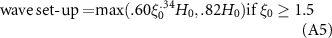
The contribution of waves to extreme water levels is parametrised for both AWLs (wave set-up) and IWLs (wave run-up). Wave run-up is defined as the height of the 2% highest excursions due to individual waves. For dissipative beaches (Vitousek et al 2017), we adopt the parameterisations from Stockdon et al (2006):


For sandy beaches, we adopt the parameterisations from Stockdon et al 2006):

For rocky dikes, we adopt the parameterisations from van der Meer and Stam (1992):


where  is the Iribarren number and
  is the deep-sea wavelength following linear wave theory. Both wave set-up and run-up are functions of deep-sea significant wave height (H0), mean wave period (Tm
) and the foreshore slope of the shoreline (βf
).
is the deep-sea wavelength following linear wave theory. Both wave set-up and run-up are functions of deep-sea significant wave height (H0), mean wave period (Tm
) and the foreshore slope of the shoreline (βf
).
For sandy beaches, we choose βf = .1 (Melet et al (2018)) as representing steep sandy beaches; this value roughly corresponds to the steepest beaches considered in the establishment of the parameterisations (Stockdon et al (2006)). For gentle rocky dikes, we use βf = 1 : 6, which is the recommended design slope for German dikes (Arns et al (2017)); and for steep rocky dikes, we use βf = 1 : 2, which is just below the steepest slopes considered in the establishment of the parameterisations (van der Meer and Stam (1992)).
: Appendix B. Doubling of AWLs and IWLs using the single variate method
To compare the results using the joint probability method to the single variate method, we have reproduced the results of figure 4 without accounting for the joint probability between waves and surges. This method is directly comparable to Vitousek et al (2017) and others. We find that doubling times are overestimated when the joint probability is not taken into account (figure B1). The joint probability of extreme waves and surges enhances the variability in extremes, and neglecting this in the statistical analysis of extremes leads to an overestimation of the amplification.

Figure B1. Doubling times derived using the single variate method for (a) Average Water Levels including wave set-up for a range of shoreline types, and (b) Instantaneous Water Levels including wave run-up.
Download figure:
Standard image High-resolution image