Relative Effects of Multiple Stressors on Reef Food Webs in the Northern Gulf of Mexico Revealed via Ecosystem Modeling

Introduction

The world’s marine and freshwater ecosystems are increasingly being affected by multiple environmental and anthropogenic stressors. In marine and estuarine systems, common stressors include overexploitation, eutrophication, hypoxia, habitat loss, pollution, acidification, harmful algal blooms, tropical cyclones, rising temperatures, and invasive species. These stressors can have system-wide impacts and affect multiple trophic levels when major energy pathways or habitat types are altered (O’Connor et al., 2009; Ullah et al., 2018), leading to changes in community structure and diversity (Flaherty and Landsberg, 2011; Worm and Lotze, 2016; Lewis et al., 2020), and impact the abundance, behavior, and fitness of individuals (Watterson et al., 1998; Hernandez et al., 2016). The effects of multiple stressors can be additive, synergistic, and/or antagonistic (Crain et al., 2008; Harvey et al., 2013; Côté et al., 2016), potentially leading to non-intuitive outcomes that make it difficult to establish causal relationships between the stressor(s) and observed responses at the level of individuals, populations, or ecosystems (Adams, 2005). The high biological complexity of many marine ecosystems can allow for compensatory responses (Ghedini et al., 2015) that make the systems more resilient to disturbance such that measurable effects may be moderated and of short duration. Furthermore, the natural variability and large observation error exhibited in marine ecosystems adds to the difficulty in detecting significant effects of multiple stressors.

Because marine ecosystems are complex and increasingly being exposed to multiple stressors, there is a critical need to understand and document how those stressors interact in order to make more accurate resource damage assessments and inform restoration efforts. Several approaches exist to understand single and cumulative impacts of environmental stressors, including experimentation, meta-analysis, mapping, qualitative/conceptual modeling, single-species modeling, and ecosystem modeling (Hodgson and Halpern, 2019). No single method can assess impacts across broad ecological scales (individual, populations, communities, and whole ecosystems), but the modeling approaches appear to have the greatest utility for addressing questions across a broad range of ecological complexities. Whole ecosystem models such as Ecopath with Ecosim (Christensen and Walters, 2004) and Atlantis (Fulton et al., 2011) have demonstrated the ability to simulate the impact of multiple stressors simultaneously to capture singular, additive, non-additive, and synergistic effects. For example, an Atlantis ecosystem model of the Chesapeake Bay (United States) was used to simulate the effects of marsh loss, submerged aquatic vegetation loss, temperature increases, and nutrient loads, both singularly and in combination (Ihde and Townsend, 2017). In the northeast Pacific, climate-induced changes to primary production, species distributions, zooplankton size structure, ocean acidity, and ocean oxygenation were simulated using a suite of Ecosim models (Ainsworth et al., 2011). A spatial-temporal ecosystem model of the NW Mediterranean was used to evaluate historical impacts of fishing, temperature, salinity, and primary production on exploited fish species (Coll et al., 2016). In each of those studies, the impacts of individual stressors were parsed out using simulation, and synergies were identified where cumulative impacts were greater than the sum of individual stressors.

Since 2010, the northern Gulf of Mexico (NGoM) has been impacted by two high profile disturbances of large spatial scale. On April 20, 2010 an explosion at the Deepwater Horizon oil rig (DWH), located about 66 km off the Louisiana coast in depths of 1,500 m, led to the largest offshore oil spill in United States history, ultimately spilling an estimated 210 million gallons of oil over the course of 87 days. The extent of the area affected by DWH included a deep sea benthic footprint of 148 km² around the wellhead (Montagna et al., 2013), a cumulative surface slick area of 149,000 km² (MacDonald et al., 2015), and 1,733 km of shoreline (Michel et al., 2013). Thus, the impacts of DWH spanned a range of biota and habitats including deep-sea corals, microbes, zooplankton, fish, shellfish, marine mammals, birds, turtles, coastal wetlands, and beaches (DWH Natural Resource Damage Assessment Trustees, 2016; Murawski et al., 2016). Notable effects of DWH on small demersal reef fish were observed near Alabama and Florida in an area impacted by the spill (88.5–85.5°W and 29–30.5°N) (Dahl et al., 2016; Lewis et al., 2020). In November 2010 (3 months after DWH ended), declines in density ranging between 35.0–95.5% were observed across seven trophic guilds of reef associated fishes, along with significant changes in fish community structure, richness, and diversity (Lewis et al., 2020).

Then, in 2011 the invasion of Indo-Pacific lionfish (Pterois volitans) expanded into the NGoM and underwent exponential population growth through 2014, eventually leading to some of the highest densities in their invaded range (Dahl and Patterson, 2014; Switzer et al., 2015; Dahl et al., 2019). Stomach contents of lionfish collected on natural and artificial reefs in the NGoM were dominated by reef-associated prey fishes such as damselfishes, cardinalfish, blennies and wrasses (Dahl and Patterson, 2014) with cases of cannibalism by lionfish confirmed with DNA barcoding (Dahl et al., 2018). In other reef ecosystems where lionfish have become established, large reductions in native fish density, biomass, and species richness were observed (Green et al., 2012; Albins, 2015). Lewis et al. (2020) hypothesized that the lack of recovery of small reef fishes in the NGoM following the DWH may be driven by top-down predation effects caused by lionfish.

Separate ecosystem models have been used in the Gulf of Mexico to evaluate the impacts of the DWH oil spill, fishing, and invasive lionfish (Chagaris et al., 2015, 2017; Ainsworth et al., 2018), but these stressors have yet to be evaluated simultaneously. The primary objective of this study was to evaluate the effect of invasive lionfish and fishing on the recovery of reef ecosystems in the NGoM following the DWH oil spill. Site-specific datasets on fish density and diet composition were used to parameterize and calibrate an Ecopath with Ecosim model of the system. The system-wide effects of each disturbance were quantified using simulated trajectories of fish biomass. We intended for this work to improve our understanding of how temperate reef ecosystems with complex food webs, like those in the NGoM, respond to broad scale stressors and advance the state of applied ecosystem modeling for resource damage assessment and restoration planning. Results of this study can be used for comparison to future field evaluations to test predicted responses of the system to combined stressors.

Materials and Methods

Study Area

We synthesized data and developed a trophic-dynamic model representative of reef food webs in an area of the NGoM extending from approximately Mobile Bay, AL in the west (−88.5°) to Choctawhatchee Bay, FL in the east (−85.5°) and from shore out to about the shelf break (latitude 29°) covering an area of 48,090 km² (Figure 1). This region of the NGoM consists of a narrow continental shelf with many artificial reefs and expansive hard-bottom habitat that support valuable commercial and recreational fisheries. The modeled area has been sampled extensively for fish abundances using a variety of gear types. Here, we utilized fish density data from an ROV-based video survey and the Southeast Area Monitoring and Assessment Program (SEAMAP) bottom trawl survey. The ROV survey has been conducted in the NGoM since 2004 to examine reef fish community, size, and trophic structure at natural and artificial reefs (Patterson et al., 2009; Dance et al., 2011), before and after DWH and the invasion of lionfish (Dahl and Patterson, 2014; Dahl et al., 2016; Harris et al., 2019). Thousands of adult reef fish and lionfish samples were also collected during the ROV survey across the NGoM to describe trophic interactions in this system, including visual stomach content analysis, DNA barcoding to identify prey items, and stable isotope analysis (Dahl and Patterson, 2014; Tarnecki and Patterson, 2015; Dahl et al., 2017; Dahl et al., 2018). The SEAMAP shrimp and groundfish trawl survey has been conducted throughout the Gulf of Mexico since 1981 during both summer and fall. These datasets were used in conjunction to estimate biomass densities and generate time series of fish abundance on reef and non-reef habitats using the ROV and trawl surveys, respectively.

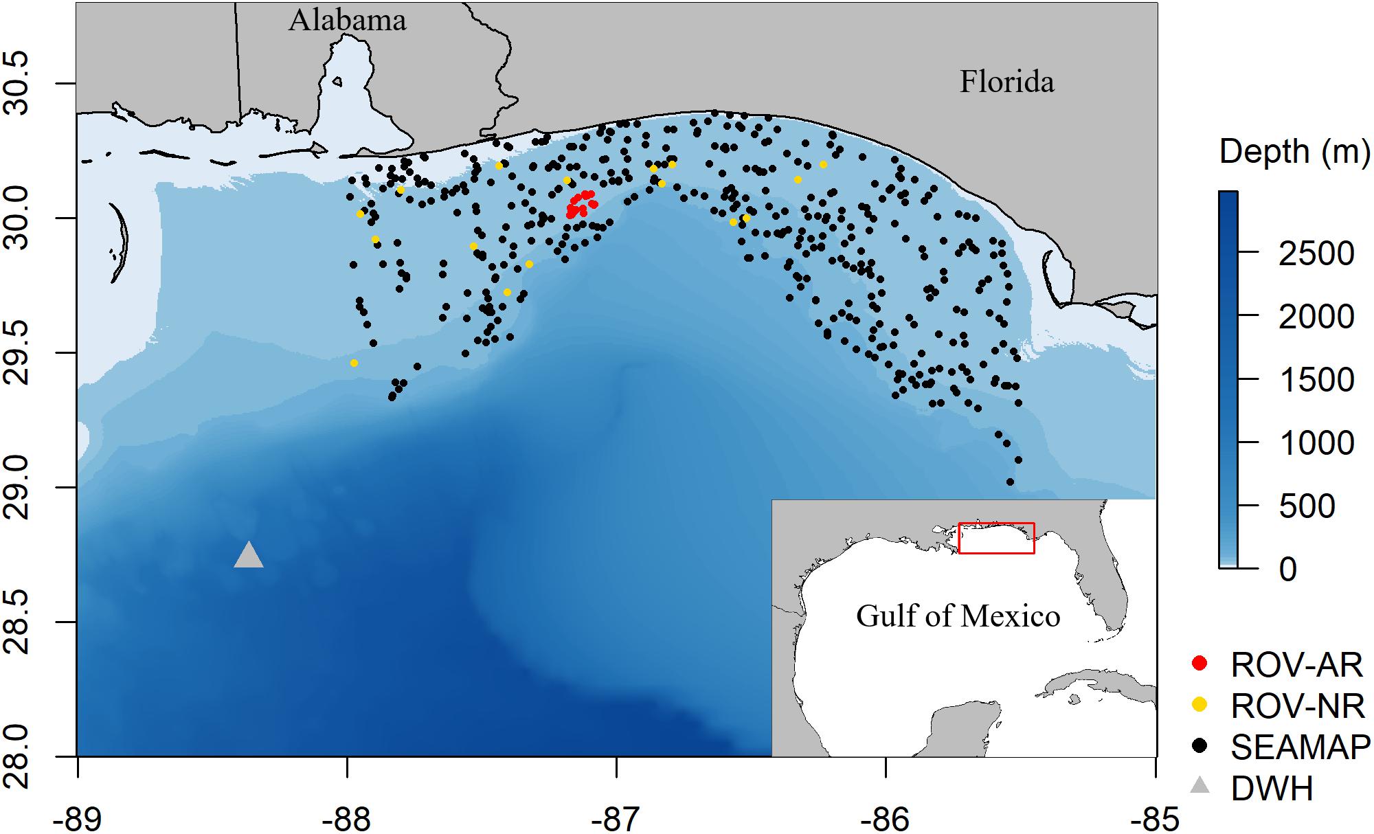
Figure 1. Map of the study region indicating natural reef (NR) and artificial reef (AR) sites sampled by the ROV survey, SEAMAP bottom trawl sites sampled from 2009 to 2016, and the location of the DWH wellhead.

The NGoM Ecosystem Model

The NGoM reef fish model was developed using the Ecopath with Ecosim (EwE) modeling software to evaluate ecosystem effects of multiple stressors in this region, including DWH and invasive lionfish. The EwE modeling package has been applied widely for analysis of aquatic ecosystems and food webs, and therefore has been described extensively and contains agreed upon best practices and diagnostic procedures (Walters et al., 1997; Christensen and Walters, 2004; Link, 2010; Colléter et al., 2015; Heymans et al., 2016). Briefly, the Ecopath component of EwE is a static mass-balance view of the ecosystem that allows for age structure representation and provides the initial state for dynamic modeling. The basic data requirements for Ecopath are biomass, total mortality (or production rate), consumption rate, diet composition, landings, and discards. In Ecosim, biomass is predicted at a monthly time step as consumption minus losses to predation, fishing, unexplained mortality, and migration (Walters et al., 1997, 2000) (Equation 1).

Here, dBi/dt represents the change in biomass B of group i over the time interval dt (1 month), g is the growth efficiency (i.e., the ratio of production to consumption rates), the first summation is the total consumption of prey j by group i and the second summation is the total consumption of group i by predators j, I represents immigration, M0 is the non-predation (“other or unexplained”) natural mortality rate, F is the fishing mortality rate, and e is the emigration rate. Consumption, Q, in Ecosim is modeled based on foraging arena theory (Walters et al., 1997; Ahrens et al., 2012), which states that some portion of prey biomass exists in arenas where predation occurs and that the transfer-rates in and out of the foraging arena, represented by the vulnerability parameter (v_ij), regulate consumption by the predator, thereby limiting the predation mortality on its prey.

Details of functional groups assignments, input parameter calculations, and data sources are provided in the Supplementary Materials and described briefly here. A total of 283 fish taxa were identified from the video-based ROV and SEAMAP trawl surveys in the study region. Those were aggregated into 14 functional groups using hierarchical cluster analysis (Gower, 1971; Rousseeuw and Kaufman, 1990) based on species attributes (e.g., growth, mortality, and consumption rates) and ecology (e.g., diet and habitat) obtained from Fishbase (Froese and Pauly, 2018) (Supplementary Table S1). Species that were dominant in lionfish diets or of importance to recreational and commercial fisheries (e.g., groupers and snappers) were included as separate biomass groups, some with multiple age stanzas. Lionfish were included as juveniles (less than 6 months and 150 mm) and adults to account for ontogenetic feeding, cannibalism by adults, and fishery selectivity. The Ecopath model consisted of 63 biomass groups including 39 fish groups, 19 invertebrate groups, 3 primary producers, and 2 detritus pools (Table 1). The model also consisted of one recreational fishing fleet, one commercial fishing fleet, and a targeted lionfish fleet (to simulate the invasions and facilitate future exploration of lionfish harvest scenarios). The Ecopath model was parameterized to reflect 2009 conditions, which is 1 year prior to the DWH disaster and the lionfish invasion.

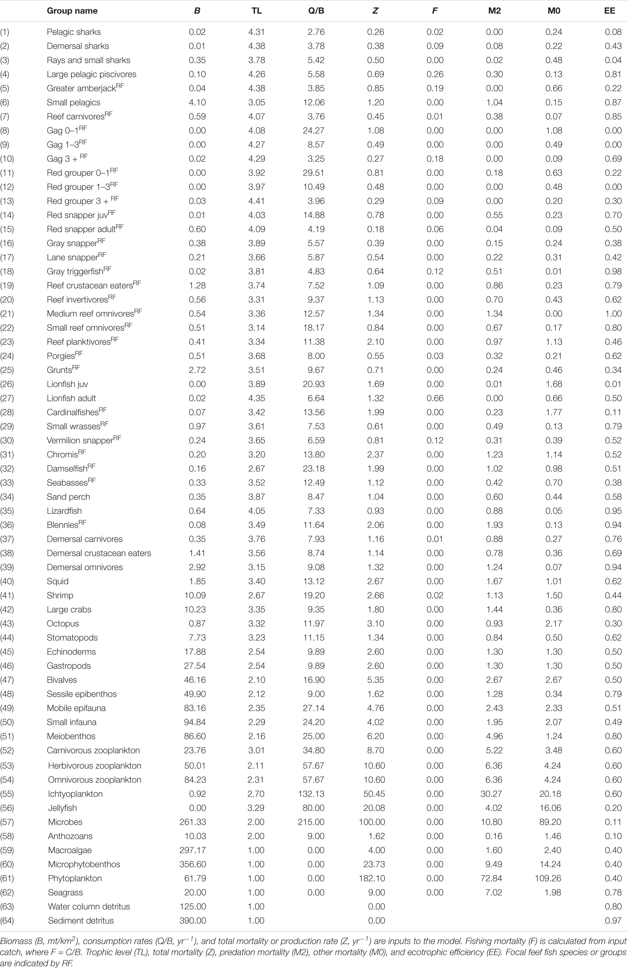
Table 1. Key inputs and outputs of the NGoM Ecopath model.

Biomass densities of fish functional groups in 2009 were estimated separately for natural reef, artificial reef, and non-reef habitats using the ROV and SEAMAP datasets and averaged together, weighted by the size of each habitat type (Table 1 and Supplementary Table S2). Production and consumption rates of fish were obtained from Fishbase. For all non-fish groups, ecotrophic efficiency (EE), which represents the proportion of production that is utilized in the system, was provided as an input and Ecopath solved for biomass (Table 1). The EE values for invertebrates, as well as their production and consumption rates, were borrowed from balanced models of the adjacent West Florida Shelf (Okey et al., 2004; Chagaris et al., 2015, 2017). Fish diet data from the ROV survey on the NGoM shelf were combined with stomach content data collected routinely by the Florida Fish and Wildlife Conservation Commission, which included some samples from SEAMAP trawls, and the Gulf of Mexico Species Interactions database, a repository of food habits data from published studies conducted throughout the Gulf of Mexico (Supplementary Tables S3, S4). Diets for invertebrate groups were borrowed from the West Florida Shelf Ecopath model (Chagaris et al., 2017). Commercial landings were obtained from the Florida FWC Trip Ticket program for the five westernmost counties on the Florida Panhandle and from NOAA Fisheries for the state of Alabama. Recreational landings were estimated from the Marine Recreational Information Program (MRIP) for the same five counties plus Alabama. After all biomass, mortality, consumption, diet composition, and landings were input, the model was mass balanced, and diagnostics were checked following Link (2010) and Heymans et al. (2016).

Accounting for Acute Mortality Associated With DWH

To account for the declines in fish abundance in 2010 associated with the DWH, a time series forcing function on the ‘other mortality’ term (M0 in Eq. 1) was developed using daily oil concentration maps (MacDonald et al., 2015), logistic dose-response curves, and observed changes in density from the surveys. Oil concentration maps were developed by converting daily percent cover maps of thin and thick surface slicks (1 and 70 μm, respectively) to oil volume (m³) and oil concentration (μg/L) assuming constant thick slickness and a volume to mass conversion of 864 kg/m³ crude oil. Daily oil concentration values from the modeled area were then averaged for each month from April to August 2010.

Generalized oil dose-response mortality curves were developed for fish, decapods, molluscs, and zooplankton based on logistic equations derived from ecotoxicology experiments conducted after DWH (Morris et al., 2015). The dose-response curves use the four parameter logistic equation to predict mortality as a function of oil concentration (Ritz 2010),

where e is the inflection point, b is the slope at the inflection point, c is the lower asymptote, d is the upper asymptote, and x is the monthly average oil concentration (μg/L) over the modeled area. Most ecotoxicology studies estimated mortality after 24, 48, 72, and 96 h of oil exposure. Exponential curves were used to extrapolate the inflection point, e, out to 720 h (∼1 month) of exposure and the b parameter was taken as the average across all experiments provided in Morris et al. (2015) within each taxa type. The steepness and extrapolated inflection parameters were calculated separately for fish (e = 3.54, b = −7.79), decapods (e = 8.14, b = −7.00), mollusks (e = 0.012, b = −5.02), and zooplankton (e = 1.05e-5, b = −5.14) and then shared across the respective model groups (Figure 2). The lower asymptote c was held constant at the Ecopath base M0 rate while the upper asymptote was set equal to some multiple, λ, of the Ecopath total mortality rate, Z. For each group with a DWH forcing function applied, the upper asymptote multipliers (λ) were estimated so that the proportional decrease in biomass was equal to that observed in the fish surveys at the end of the DWH event (i.e., August 2010). Essentially, this approach modified the generalized dose-response curves for each species or model group in order to approximate the observed biomass declines following DWH, assuming all other mortality agents were constant.

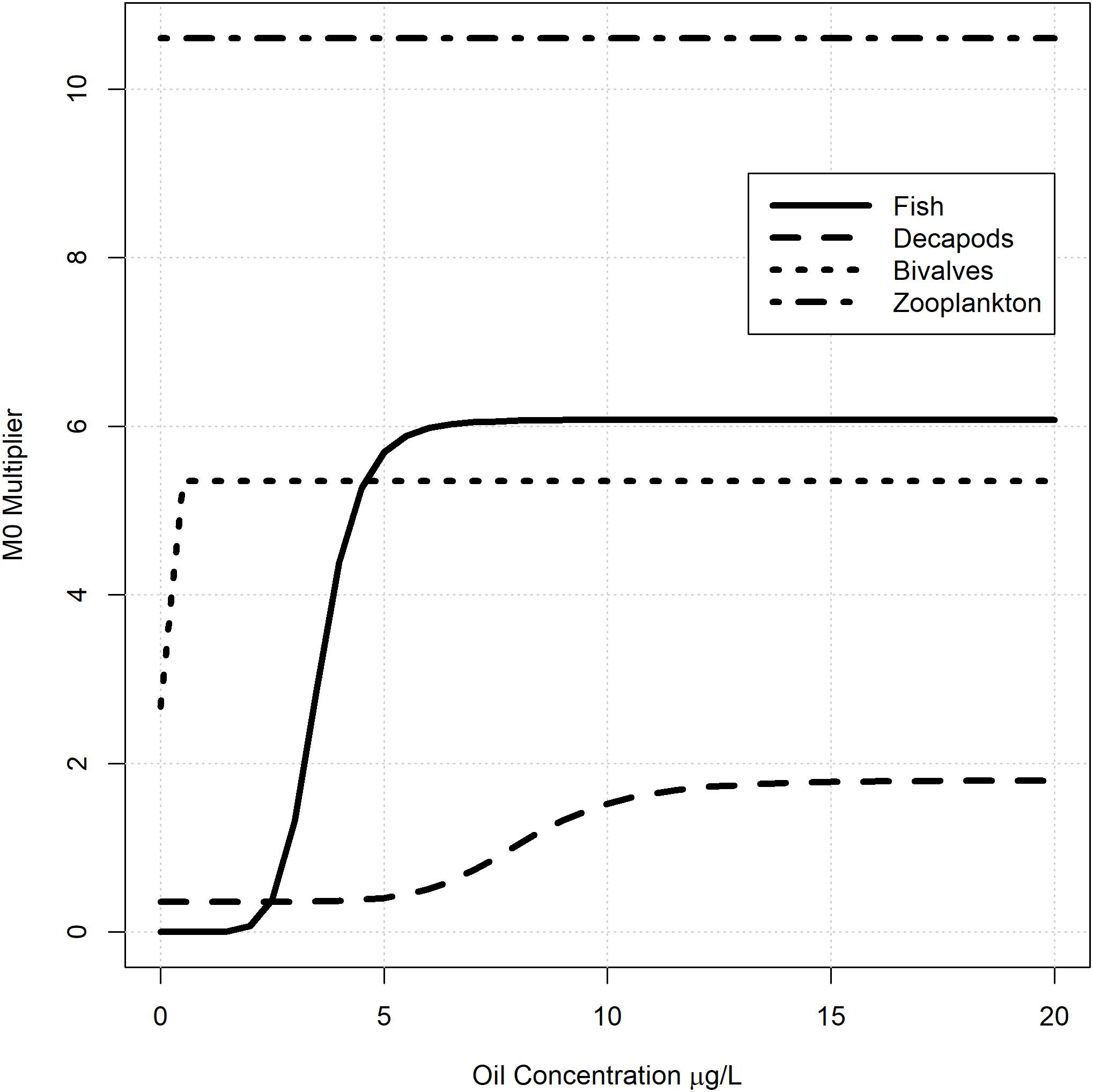
Figure 2. Generalized oil mortality response curves used in the NGoM Ecosim model to simulate mortality associated with the Deepwater Horizon oil spill. The generalized curves are based on data from Morris et al. (2015) and were modified for each fish group in the model by increasing or decreasing the upper asymptote.

The DWH M0 forcing functions were developed outside the ecosystem model and input as a monthly time series of multipliers on the ‘other mortality’ term. During the months before and after the DWH, the M0 multiplier was set equal to 1. For April-August 2010, monthly M0 was estimated using the modified logistic dose-response curves (Eq. 2) and the time series of monthly oil concentration. Forcing functions were applied to 40 model groups including all zooplankton, invertebrates, small demersal fishes, and large bodied fish exhibiting declines following DWH.

Simulating the Lionfish Invasion in Ecosim

There are several potential approaches to simulate species invasions in EwE (Langseth et al., 2012). We followed an approach in Langseth et al. (2012) as adapted by Chagaris et al. (2017) to simulate the invasion of lionfish in Ecosim. This required initializing Ecopath with a negligible biomass of lionfish representative of 2010 densities measured during the early detection phase of the invasion, a positive biomass accumulation rate parameter (BA = 0.8), and a hypothetical fishing fleet to maintain lionfish biomass at initial levels prior to the invasion. Landings of lionfish were entered into Ecopath, such that fishing mortality was equal to natural mortality (F = M = 0.66 yr^–1) and the input total mortality rate Z was doubled (i.e., Z = F + M = 1.32 yr^–1). In Ecosim, the invasion is suppressed during the first 2 years of simulation (2009–2010) by doubling the Ecopath fishing mortality on lionfish. Lionfish are then allowed to increase beginning in 2011 (after DWH forcing) by setting lionfish effort to zero to reduce Z to M (i.e., Z = M when F = 0). This method is preferred because Ecopath is initialized with a pre-invasion biomass that does not create mass imbalance in the model and allows for estimation of lionfish vulnerability parameters, vij, that regulate top-down predation impacts by lionfish on their prey.

Ecosim Model Calibration

The NGoM Ecosim model was calibrated to time series of relative abundance from the ROV and SEAMAP surveys of fish densities in the study region, standardized using a delta generalized linear modeling approach (Lo et al., 1992; Maunder and Punt, 2004). In total there were 45 reference time series of fish and macro-invertebrate relative abundance indices derived from these two surveys. Forcing time series included observed commercial and recreational catches, satellite derived chlorophyll-a (as a proxy of phytoplankton productivity), satellite derived particulate organic carbon (POC, as a proxy for water column detritus), and the DWH M0 forcing functions described above. Chlorophyll-a and POC time series are the monthly area averages for the model spatial domain, derived from composite MODIS Aqua satellite imagery (Acker and Leptoukh, 2007). With these forcing functions in place, the model was calibrated to fit the time series of relative abundance.

In Ecosim, there are two sets of parameters describing the foraging arena consumption model which must be calibrated to fit the observed data. The first set of Ecosim parameters are the vulnerability exchange rates, vij, and there is one parameter for each predator-prey interaction. The Ecosim v_ij parameters are input as multipliers on Ecopath base predation mortality rates (M2_ij) to represent the maximum possible predation mortality rate that can be exerted on a prey item at high predator biomass. The second set of Ecosim parameters include maximum P/B, foraging time adjustments (FTA), predator effect on foraging times, and prey switching. In general, these parameters define the shape of predator-prey functional responses and can be changed to represent stronger density dependent effects and risk-sensitive foraging strategies. While these parameters can strongly influence the model, they are not estimable in Ecosim and it has been recommended that simulations should include a range of parameter combinations to better reflect ecological uncertainty and sensitivity to perturbations (Gaichas et al., 2012).

The Ecosim model was fitted by estimating v_ij values that minimized the weighted sum of squared (SS) deviations of log biomass and log predicted biomass, where observed relative abundance indices are scaled internally by the maximum likelihood estimate of a scaling factor, q, times the Ecopath absolute abundance. The most sensitive v_ij parameters were first identified by adjusting each v_ij slightly (±10%), one at a time, to see how much the SS changed. As a conservative approach, it has been recommended to only estimate K − 1 parameters (Heymans et al., 2016), where K is the number of calibration time series used to fit the model (K = 44 for the NGoM model). After the v_ij sensitivity search was completed, the K − 1 most sensitive v_ij parameters were then “turned on” for estimation, implemented in Ecosim using a Marquardt non-linear search algorithm. Ecosim models are prone to local minima in SS, thus requiring repeated searches in order to find model convergence. Therefore, the v_ij sensitivity search and estimation procedure was repeated until no further improvement in the SS was obtained. At each iteration, the model may identify and estimate a different set of K − 1 v_ij, such that the total number of v_ij estimated after convergence is greater than K − 1.

The NGoM Ecosim model was fitted under seven alternative parameter configurations for prey switching and foraging time adjustments (Table 2). We were especially interested in evaluating the effect of prey switching by lionfish because we found the model to be sensitive to this parameter in initial test runs. Prey switching is said to occur when predator diet proportions change more rapidly (or slowly) than relative abundances. This is modeled by modifying the rate of effective search (a_ij) in relation to changes in abundance of prey using a power function $a_{\text{ijt}}=a_{\text{ij}}\cdot B_{\text{i}}^{P_{\text{j}}}$, where P_j = [0,2]. The default configuration (mod1) included foraging time adjustment for the youngest age of all multi-stanza groups (FTA = 0.5) to allow for compensatory improvements in juvenile survival at low stock sizes, FTA = 0 for all other groups, and prey switching turned off (P_j = 0, Table 2). In configurations 2–4, prey switching by lionfish was set to values of 0.5, 1, and 1.5, respectively (with default FTA settings), which provided sensitivity analysis for prey switching intensity on model predictions. Models 5 and 6 both included FTA of 0.5 for all consumer groups (and P_j = 0), with model 6 including risk-sensitive foraging by setting the predator effect on feeding time equal to 1 for all groups (Table 2). The estimated vulnerability parameters were conditioned on the chosen values for prey switching (or FTA), so that each model was recalibrated using the repeated search procedure described previously. Lastly, model 7 represented a combination of the previous models, arrived at by evaluating the individual SS components across models 1–6 (Supplementary Table S5) and assigning the best fit parameter settings. This was followed by the repeated search procedure and iterative manual adjustments to both FTA and v_ij in order to move the model away from local minima.

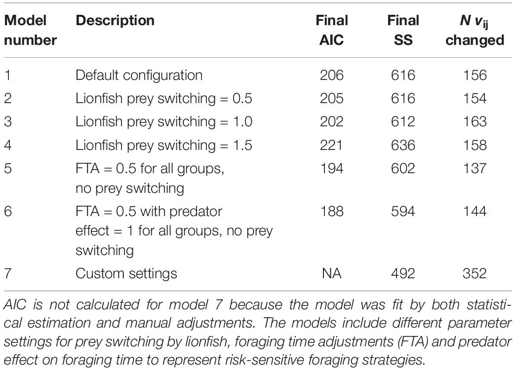
Table 2. Ecosim model configurations with final AIC and SS values after the repeated sensitivity search and v_ij estimation.

Model Scenarios

For each of the seven NGoM Ecosim model configurations we evaluated eight stressor scenarios over the time period 2009–2016. These included the “full” model with catch (C), lionfish (LF), and DWH (C + LF + DWH), the “null” model with no stressors applied, and all singular and paired combinations (C, DWH, L, C + DWH, C + LF, and LF + DWH). The full model (C + LF + DWH) is equivalent to the baseline scenario fitted to time series data. In the scenarios without lionfish, the invasion was suppressed by maintaining high fishing mortality on lionfish beyond 2010 and multiplying the v_ij of lionfish prey by 0.10, essentially causing lionfish to become extinct in the model. To exclude DWH effects, the M0 forcing function time series were reset to 1 so as not to cause any added mortality between April and August 2010. In the scenarios without fishing catch and effort time series forcing values from 2010 to 2016 were maintained at 1% of the 2009 value. In total, we simulated 8 stressor scenarios across all 7 model configurations for a total of 56 Ecosim runs.

Analysis of Model Output

For each stressor scenario and model configuration, we output the monthly biomass trajectories for each model group and calculated community metrics for the native reef fish community identified in Table 1 (excluding lionfish) at each model time step. Although biomass dynamics were predicted for all model groups, including invertebrates and primary producers, we focused our analysis on the reef fish community because they contain informative data spanning the period before and after the DWH and lionfish invasion on which we can evaluate model performance; and also because reef fishes and their habitats were prioritized for restoration funds following the DWH, with at least $200 million USD allocated to research, monitoring, and enhancement of these resources since 2010¹. To determine which stressors, or combinations thereof, had the strongest effects on simulated biomass, and to visualize species similarities, we used redundancy analysis (RDA) as implemented by Legendre and Legendre (2012) in the R vegan package (Oksanen et al., 2019). The RDA is a canonical ordination technique commonly used in ecology to model multivariate response data (Legendre and Gallagher, 2001) that requires a response matrix Y, typically representing species abundances across sites, along with a matrix of explanatory variables X measured at each site. In this context, we assigned the Y matrix as the species terminal month biomass, standardized to the maximum terminal month biomass for each species across all model configurations and stressor scenarios, and the explanatory variable is the stressor scenario. We reversed the sign of the response variable prior to running the RDA so that the species would be ordinated in proximity to the explanatory factor with the strongest negative effect. The terminal month biomass was chosen because we were most interested in the recovery status at the end of each scenario in order to understand the effect that each stressor and combination of stressors had on the ecosystem 6 years after the DWH and 5 years after the lionfish invasion. To simplify interpretation, we applied RDA to just 27 model groups using output from all 7 model fits (i.e., the ‘replicates’) in order to capture the variation associated with the different Ecosim parameter combinations in the ordination. The 27 model groups used in the RDA represent the reef fish and demersal species or functional groups (excluding lionfish and juvenile stanzas) for which we were most interested and that also contained informative time series for model fitting.

Reef fish community metrics included total reef fish biomass, mean trophic level of reef fishes weighted by their biomass, and reef fish diversity expressed as Shannon’s diversity index (H) and Kempton’s Q-90 with the exclusion threshold set at 50% of the starting biomass (Ainsworth and Pitcher, 2006). Kemptons’s Q-90 is a modified form of Kempton’s Q index (Kempton and Taylor, 1976) that uses the slope between the 10^th and 90^th percentile rather than the slope of the interquartile range. The Q-90 diversity index is better suited for ecosystem simulation models that typically use functional groups of aggregate species and ignore rare species, and therefore do not result in long tails in the cumulative biomass distribution as would be expected for datasets containing low abundance species.

Results

Model Performance

The seven Ecosim configurations all produced similar fits to the data (Figure 3) indicating that the model was fairly robust to assumptions about prey switching and foraging time adjustments. Of the strictly estimated models (models 1–6), SS ranged from 594 to 636, AIC was between 188 and 22, with model 6 having the lowest AIC (Table 2). Convergence in the model was usually obtained after 10 iterations of the v_ij sensitivity search and estimation procedure (Supplementary Figure S1), resulting in 137–163 v_ij’s estimated by the model (Table 2). The manually tuned model (model 7) resulted in the lowest overall SS of 492, with most of the improvements coming from better fits to blennies (Blenniidae), demersal carnivores, demersal omnivores, lionfish, and chromis (Chromis spp.) (Figure 3 and Supplementary Table S1).

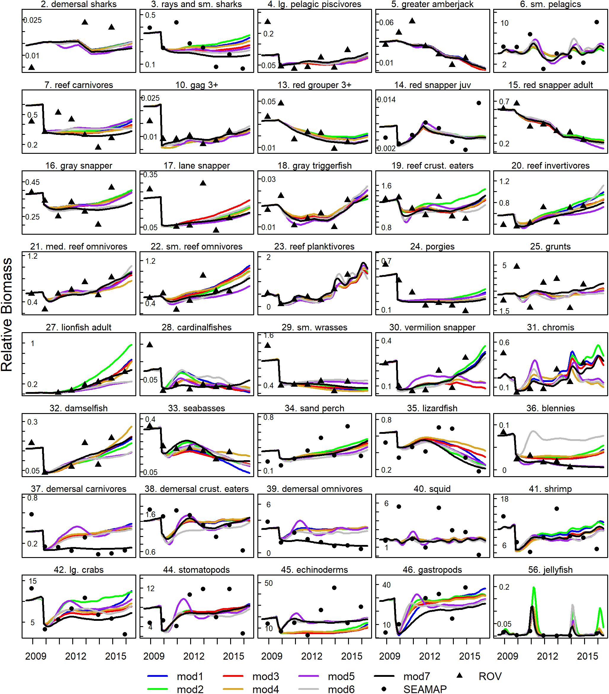
Figure 3. Ecosim predicted (lines) and observed (points) relative biomass from the seven fitted Ecosim models.

Model 7 represented a combination of parameter settings from models 1–6, arrived at by evaluating the SS contribution across groups and applying the setting with the lowest SS for each group. For example, model 2 had the best fit to lionfish biomass with prey switching set at 0.5, and blennies were best fit in model 5 with an FTA of 0.5. In the end, model 7 included FTA = 0.5 for 30 out of 58 consumer groups, predator effect on feeding time for 19 of those groups, and lionfish prey switching of 0.5. Finally, after 10 repeated searches in model 7 we found that demersal carnivores and demersal omnivores were trapped in a local minimum with vulnerabilities near 1.0. Therefore, we reset the v_ij of all prey items for those groups to 10 before conducting the final vulnerability search estimations, which moved the SS considerably lower than estimated in the prior iterations (Supplementary Figure S1). Visual inspection of the fits to observed abundance data showed that the Ecosim model was capable of reproducing observed trends in abundance across a broad range of species and functional groups, and that alternative model configurations resulted in some variability in biomass trajectories but in most cases did not result in drastically different predictions (Figure 3). Thus, the model fit the observed trends in abundance well and was robust to assumptions made about input parameters.

Simulated Changes in Fish Biomass

Patterns in simulated biomass trajectories exhibited divergence across species/functional groups and stressor scenarios (Figure 4), which was due to singular and cumulative impacts of stressors as well as direct and indirect effects arising through food web interactions. For harvested species (e.g., snappers, groupers, and greater amberjack), the lowest terminal year biomass occurred in the multiple stressor scenarios that included catch (C + L and C + L + DWH). Biomass of lionfish prey items, such as seabasses (Serranidae), chromis (Pomacentridae), and lizardfish (Synodontidae), converged at about the same value in all scenarios that included lionfish, regardless of whether DWH or fishing effects were present or not. In other instances, biomass trajectories did not converge with other stressor scenarios during most of the simulation time period. This was the case for juvenile red snapper (Lutjanus campechanus), small reef omnivores (Acanthuridae, Chaetodontidae, Ephippidae, Monacanthidae, and Pomacanthidae), cardinalfishes (Apogonidae), and vermilion snapper (Rhomboplites aurorubens) and indicates the incremental cumulative effects that each stressor had on those species.

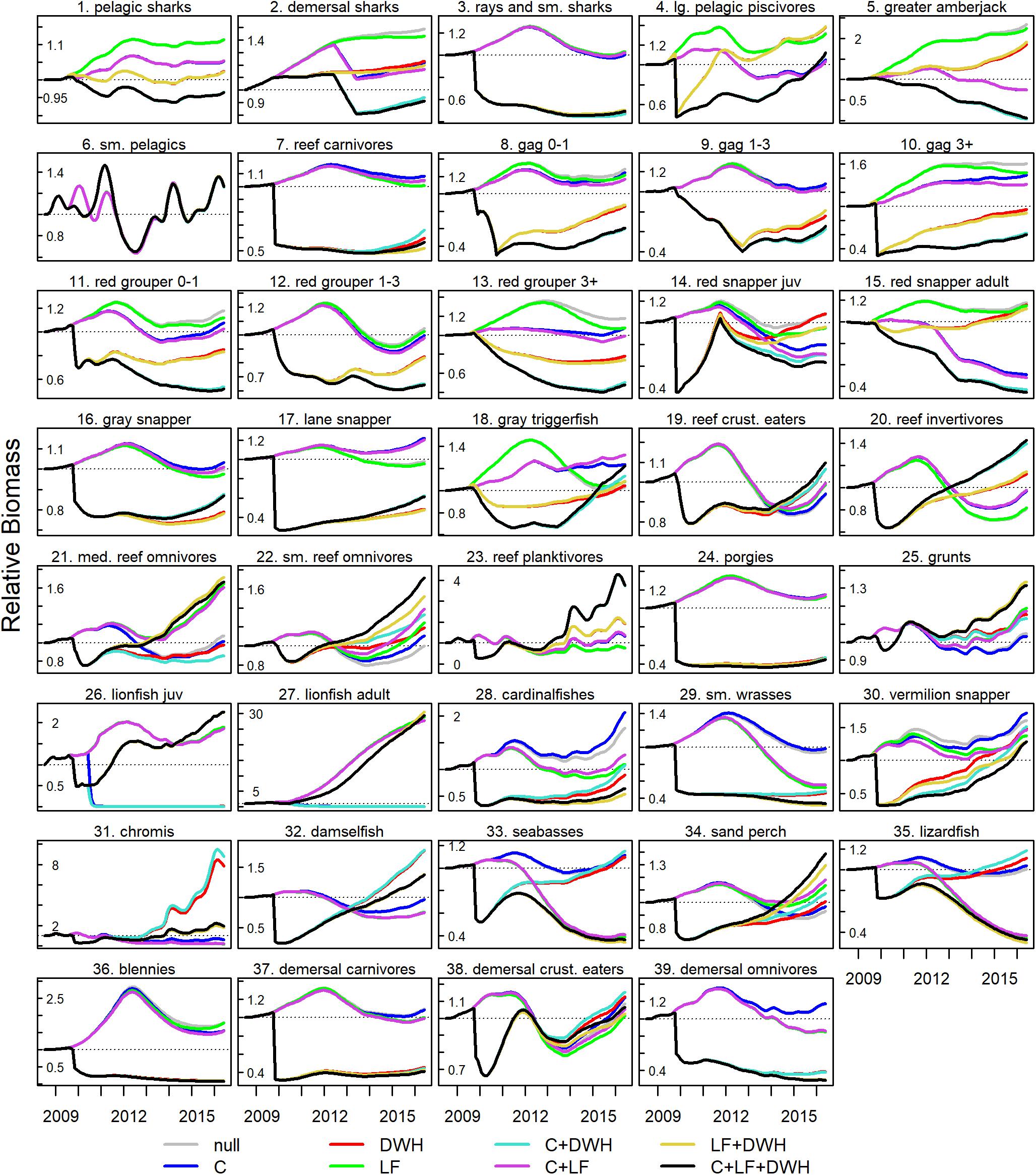
Figure 4. Ecosim biomass trajectories under 8 stressor scenarios, including combinations of catch (C), Deepwater Horizon (DWH), and lionfish (LF). Displayed are a subset of modeled fish groups from the best fit model 7. Biomass trajectories for all functional groups are available in the Supplementary Materials.

In the redundancy analysis, stressor scenario explained 74% of the variation in simulated terminal biomass data, with the first two axes explaining 58% of that variation, and the third axis (not shown) explaining 15% of the variation (Figure 5). The first axis was strongly influenced by the combination of C + LF + DWH stressors in the negative direction and C and the null treatment in the positive direction, while the second axis is influenced by LF in the positive direction and by the combined effects of C + DWH in the negative direction. The RDA biplot also shows the relationship between stressors and the terminal month biomass of each species or functional group. The angles in the biplot between the arrows pointing to the species and the stressor, and between the species themselves or the stressors themselves, reflect their correlations. Therefore, the RDA biplot allows us to visualize similarities among species/functional groups, similarities among stressors, and the correlation between stressor combinations and functional groups.

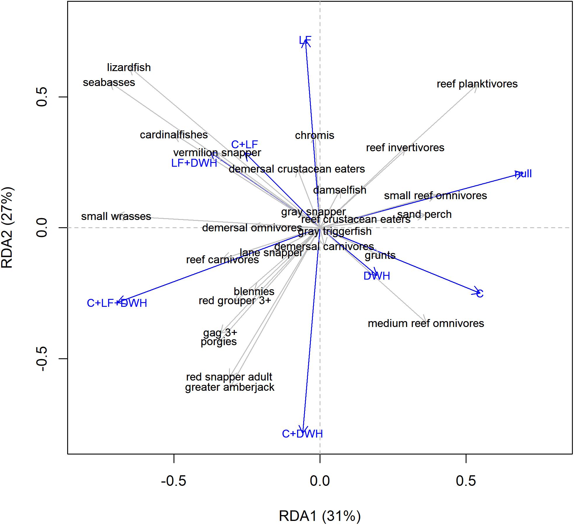
Figure 5. Redundancy Analysis (RDA) biplot (Axis 1 and 2) of modeled terminal year biomass showing 27 focal reef or demersal fish species/functional groups and stressor scenarios. Stressors include all combinations of catch (C), Deepwater Horizon (DWH), and lionfish (LF).

The model showed that the combined effects of fishing, DWH, and lionfish were similar for reef fish species of economic importance, such as red snapper, greater amberjack (Seriola dumerili), red grouper (Epinephelus morio, and gag (Mycteroperca microlepis) that experienced biomass declines in 2010 due to DWH and did not recover substantially over the simulated time period (Figure 3). In the bottom left quadrat of the RDA biplot, these species are in close proximity and therefore had lowest biomass in the C + LF + DWH and C + DWH scenarios (Figures 4, 5). The location of these groups midway between those 2 stressor scenarios (one without lionfish) indicates that the correlation to those two stressors is about equal and that lionfish had little influence on simulated biomass of those species. However, the combined effect of catch with lionfish and DWH did result in slight reductions in juvenile red snapper biomass for model 7 (Figure 4). Blennies and porgies (Sparidae) are also located in this quadrat and near the two grouper species along the first two axes (Figure 5). But unlike the groupers, blennies and porgies are negative on the third axis, with RDA3 scores of −0.24 and −0.48, which is strongly influenced by the DWH (RDA3 = −0.71) and LF + DWH (RDA3 = −0.52) scenarios.

In the top-left quadrat of the RDA biplot are the species or functional groups that were strongly influenced by the presence of lionfish (Figure 5). These include lizardfish, seabasses, cardinalfishes, and vermillion snapper, which are all positioned in proximity to one another between the centroids of LF + DWH and C + LF scenarios. The small wrasses (Labridae) group is isolated at the left end of axis 1 almost equally between LF + DWH and C + LF + DWH, indicating that the cumulative effect of lionfish and DWH is the primary driver on this group (Figure 5). In contrast, chromis are oriented at almost the exact same angle as the LF only scenario, and away from any of the combined stressor scenarios, illustrating that the singular effect of lionfish had the strongest influence over this group (Figures 4, 5).

The small demersal reef fishes in the right two quadrats of the biplot experienced biomass responses that were confounded by indirect trophic interaction effects. Reef planktivores (Clupeidae, Engraulidae, Priacanthidae, and Serranidae) and reef invertivores (Chaetodontidae, Cynoglossidae, Diodontidae, Pomacanthidae, and Tetraodontidae) are positioned in proximity to one another and nearly equally between the null and LF centroids, meaning that these groups benefited from reduced top-down predation and competition as a result of fishing and DWH stressors. However, they are also positioned high on the second axis indicating that they experienced direct negative effects of the lionfish invasion (Figures 4, 5). Small reef omnivores and sand perch (Diplectrum spp.) were predicted to respond similarly to each other (Figure 4) and are therefore in close proximity along the first two axes and oriented at nearly the exact same angle as the null scenario and influenced less by lionfish (Figure 5). Whereas, medium reef omnivores (Chaetodontidae, Monacanthidae, Ostraciidae, Serranidae, and Sciaenidae)are positioned on the right of axis 1 and negative on axis 2, suggesting that they were negatively affected by C + DWH, but positively affected by the presence of lionfish (Figures 4, 5). Lastly, the species and functional groups clustered around the middle of the biplot are those whose terminal biomass was predicted to converge across all scenarios. This indicates that the presence of lionfish, fishing, and/or DWH did not substantially affect those groups and that they may potentially have high resiliency to these stressors.

Terminal biomasses from all 7 model configurations were included in the RDA analysis to capture the variation associated with Ecosim model parameterization. For the stressor scenarios applied here, there was strong coherence in biomass dynamics across all model configurations with only a few exceptions (Supplementary Figures S2–S9). Cardinalfish had the highest variation in terminal year biomass for the C + LF and LF only stressor scenarios, with coefficients of variation (cv) equal to 1.22 and 1.16, respectively, while the cv in all other stressor scenarios ranged between 0.17 and 0.48. Vermilion snapper, seabasses, and lizardfish also had high variation (cv’s between 0.50 and 0.67) in the C + LF and LF only scenarios. Chromis exhibited high variation in the C + DWH (cv = 0.78) and DWH only (cv = 0.72) stressor scenarios, while blennies had cv’s of about 0.65 in the four stressor scenarios that included DWH impacts. For all other groups and stressor scenarios, the cv associated with model configuration was less than about 0.4 with a mean of 0.13.

Impacts on Reef Fish Community Structure

The impact of each stressor on community structure was evaluated using aggregate biomass, trophic, and diversity metrics. Total reef fish biomass was 10.45 g/m² at the start of the simulations and declined to approximately 7.30 g/m² immediately after the DWH, increasing over time to 11.80 g/m² in the full (i.e., observed) scenario that included all three stressors (Figure 6A). The only scenarios with higher terminal year biomass were C + DWH (12.60 g/m²) and the DWH only (11.92 g/m²) scenarios, indicating higher biomass in absence of lionfish impacts and fishery removals. The other three scenarios that included lionfish all fell below the full model with ending biomasses of 11.21, 10.77, and 10.66 for LF + DWH, C + LF, and LF scenarios, respectively. The mean trophic level of reef fish was 3.58 at the start of the simulation and then varied over time between the range of 3.42 and 3.65 across all scenarios and models (Figure 6B). The effects of stressor scenarios on reef fish trophic level were generally opposite those of biomass, such that high biomass predictions coincided with biomass increases in lower trophic levels species. Reef fish diversity at the start of simulation, as indexed by Shannon’s H and Kempton’s Q-90, were 2.54 and 3.48, respectively (Figures 6C,D). Both diversity measures remained at about this level for the duration of the simulation under the null and fishing only scenarios. In the C + LF and LF scenarios, diversity declined gradually over time as lionfish invaded the system, eventually ending at H values of 2.46 and 2.44 and Q-90 values of 2.99 and 3.15 for the C + LF and LF only scenarios, respectively. For the DWH scenarios, diversity was sharply reduced in 2010 before increasing over the remainder of the simulation. However, the presence of lionfish resulted in lower H values (2.33 and 2.35 for C + LF + DWH and LF + DWH, respectively) than those without lionfish (2.45 and 2.47 for C + DWH and DWH, respectively). The increase if reef fish biomass paired with low diversity in the C + LF + DWH and LF + DWH scenarios indicates that biomass recovery did not occur across all trophic groups.

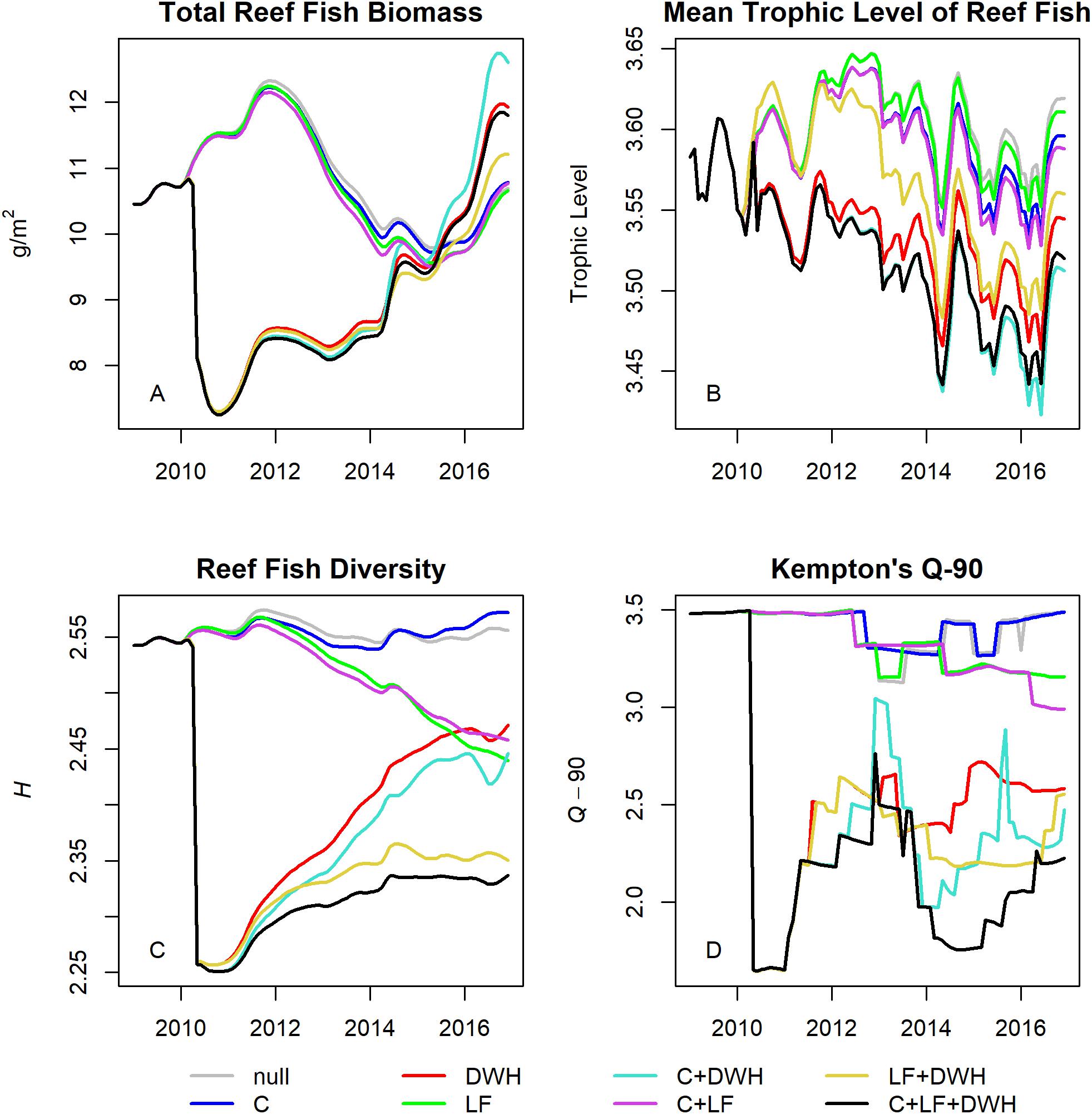
Figure 6. Community metrics calculated with output from stressor scenarios using the best fit model 7. Total biomass (A), mean trophic level (B), Shannon’s diversity (C), and Kempton’s Q-90 (D) were calculated for the reef fish species/functional groups identified in Table 1.

Discussion

Using data synthesis and a trophic dynamic model of the NGoM, we were able to evaluate the effects of multiple stressors on reef ecosystems in this region. The DWH oil spill, invasion of Indo-Pacific lionfish, and fishery exploitation, have each impacted the system but in fundamentally different ways. The DWH oil spill was a relatively acute event that directly affected the entire ecosystem, including plankton, benthic invertebrates, demersal fishes, and upper trophic level reef fishes. The lionfish invasion directly impacted small demersal fish species in all years after the DWH through top-down predation control, but also affected other species via competition for prey. Lastly, fishing effects were limited to relatively few, mostly upper trophic level fishes over the entire time period of simulation and is responsible for poor recoveries in those species after DWH. Therefore, our results showed that the NGoM food web was strongly impacted by the acute effects of the DWH event and the multi-year impacts of the lionfish invasion, and that the lionfish invasion suppressed recovery of several small reef and demersal fishes following the DWH event. Overall, this simulation exercise enabled us to remove the effects of a given stressor (i.e., DWH, lionfish, or fishery exploitation) to evaluate the impacts on different reef fish taxa, and examine why different taxa have shown different recovery trajectories in the decade since the DWH (Lewis et al., 2020).

The model predicted that most species or functional groups had lower biomasses when two or more stressors were applied simultaneously (more species were negative along axis 1 in Figure 5), while a few species were predicted to have higher biomass under those same scenarios due to lower abundances of predators and competitors. This result is not atypical of complex food web models which often predict indirect effects and unintended consequences associated with trophic relationships (Walters et al., 2008; Pine et al., 2009; de Mutsert et al., 2016, 2017). However, it is possible that some of the unexpected positive effects from the lionfish invasion predicted by the NGoM Ecosim model are due to model structure. For example, one criterion for parsing out model functional groups was importance of fish in lionfish diets. This resulted in several functional groups that, by design, did not have strong direct ties to lionfish (groups 20–23), and therefore benefited indirectly in the invasion scenarios.

The DWH oil spill effects were simulated in the NGoM Ecsoim model by applying a series of externally estimated multipliers to the other mortality (M0) term in the biomass dynamic equations. This approach was successful in replicating the observed changes in fish density in 2010 from the ROV survey. However, no sublethal or persistent effects on growth or reproduction were considered nor were the impacts of oil dispersants. Laboratory exposure studies conducted on larvae and juvenile fish after the DWH consistently demonstrated adverse effects of PAH on vascular, hepatosomatic, and epithelial systems leading to reduction in growth and survival (Brewton et al., 2013; Incardona et al., 2014; Brown-Peterson et al., 2015; Esbaugh et al., 2016). There have been far fewer field studies that documented long-term effects and reduced growth in fishes following the DWH. Incidences of PAH-induced skin lesions on bottom-dwelling species, including red snapper, collected on the continental shelf edge just north of the DWH site were higher 1–2 years after the DWH (Murawski et al., 2014), and incremental otolith analysis found slower growth-at-age of red snapper over the same time period (Herdter et al., 2017). But there is no evidence to suggest that the DWH had widespread impacts on growth of post-juvenile fishes. A Gulf of Mexico Atlantis ecosystem model (Ainsworth et al., 2018) also used modified dose-response curves to estimate mortality and growth rate modifiers, along with a depuration model to account for persistent effects of exposure. However, the more elaborate representation of oil spill effects in Atlantis did not result in appreciably better fits to the ROV reef fish community data than did the NGoM Ecosim model.

The NGoM Ecosim model was able to accurately predict the trend in observed lionfish densities from 2009 to 2016. In a previous Ecosim model of the lionfish invasion on the neighboring West Florida Shelf (Chagaris et al., 2017), the foraging arena vulnerability parameters were not estimated due to lack of informative time series data. Invasion scenarios were instead evaluated over a range of vulnerability settings, which led to drastically different simulated invasion trajectories. In this application, observed densities of lionfish and their prey were available from the site-specific ROV survey, enabling the model to estimate the vulnerability parameters statistically and giving more confidence in the predicted impacts. In a lionfish modeling study on a Caribbean coral reef (Arias-González et al., 2011), the predicted impacts were similar to ours, with both positive and negative responses for different functional groups due to direct top-down predation and competitive interactions. It has been speculated that the reductions in fish biomass and diversity caused by DWH increased vulnerability to the lionfish invasion (Murawski et al., 2016). However, the NGoM Ecosim model predicted the contrary, with slightly slower population increase for lionfish when DWH was included, due to reduced availability of prey during the first few years of the invasion. Lionfish densities measured by the ROV survey in 2018 declined by 75–80% on natural and artificial reefs and were believed to be associated with an ulcerative epizootic skin disease (Harris et al., 2020). Due to their high densities and low genetic diversity, it is hypothesized that disease transmission is density-dependent, and the population may continue to fluctuate over time. While the NGoM Ecosim model does include density-dependent population control of lionfish through cannibalism (Dahl et al., 2018) and competition for food, future simulations of lionfish population dynamics should account for this recently discovered disease.

There is considerable uncertainty in the fisheries catch data used in this model because the commercial and recreational landings data did not contain georeferenced information about where fish were caught. Thus, we were unable to parameterize the model with accurate catch data exclusively from within the model’s spatial domain. Furthermore, recreational catch and discards are estimated from a creel survey, sometimes with very low precision, depending on the species and region. Despite these data uncertainties, the site-specific fishery exploitation rates estimated by the NGoM Ecosim model for key fishery species were well within reason when compared to recent stock assessments or empirical estimates. For example, red snapper Ecosim exploitation rates ranged from 0.10 to 0.65, while the exploitation rates from a tagging study conducted in the NGoM were estimated between 0.14 and 0.37 (Sackett et al., 2018). Ecosim exploitation rates for gag were estimated between 0.08 and 0.41, while the most recent stock assessment estimated exploitation rates of 0.07–0.34 y^–1 over the same time period (SEDAR, 2016). Gray triggerfish exploitation rates from the stock assessment model were estimated to be 0.07–0.13 y^–1 (SEDAR, 2015) and Ecosim estimated exploitation rates of 0.12–0.30 y^–1. This gives us confidence that the catch forcing time series used in the model are compatible with the density estimates, and the scenarios with and without catch likely resulted in expected population responses to fishing. For other non-target species (e.g., grunts and reef carnivores) the Ecosim exploitation rates are low (<0.05 y^–1), and while there are no alternative estimates for comparison, it is reasonable to assume these estimates are low compared to the aforementioned target species.

Conclusion

This study demonstrated the potential for complex responses in disturbed reef ecosystems of the northern Gulf of Mexico. We use a highly simplified model that only represents a small fraction of the variability and stochasticity present in the system. Therefore, we can safely assume the predictions are well within the realm of possibilities that might arise in a far more complex system. The model makes several key predictions. First, it shows us that lionfish have had a major impact on this ecosystem, leading to slower recoveries following DWH and lower fish biomass and diversity. Continued investment in monitoring and mitigation strategies is therefore warranted. Second, the model predicted that some species or functional groups would have recovered to their pre-DWH biomass within 2–3 years, while others would not have recovered at all, regardless of lionfish. This suggests that the ecosystem possibly underwent some level of reorganization, preventing it from returning to its pre-spill state. Lastly, the model predicted fishing to be the major driver for a suite of upper trophic level species, and that cumulative effects of fishing with other stressors can result in further biomass declines. Therefore, harvest policies based on single species projections alone may not perform as expected when other threats are present. Combined, these results highlight the need for ecosystem approaches in resource damage assessment and fisheries management to identify causality across multiple stressors and develop robust harvest policies.

Data Availability Statement

Publicly available datasets were analyzed in this study. These data can be found here: ROV fish abundance data are available on the GRIIDC repository DOIs: 10.7266/N77H1H5; 10.7266/N7XS5SZ; and 10.7266/N7T1526. Ecopath model inputs are available on the GRIIDC repository DOI: 10.7266/N77D2SG. SEAMAP trawl data are available on the Gulf States Marine Fisheries Commission data server www.gsmfc.org/seamap.php. Gulf of Mexico Species Interactions Database http://gomexsi.tamucc.edu/. Satellite data were available from NASA Giovanni website https://giovanni.gsfc.nasa.gov/giovanni/. Ecotoxicology data were made available by NOAA’s Deepwater Horizon Trustee Toxicity Testing Program https://www.diver.orr.noaa.gov/dwh-toxicity-studies.

Author Contributions

DC, WP, and MA designed the study. WP collected and provided fish abundance and diet data. DC developed the ecosystem model. MA helped structure the model scenarios. All authors contributed to writing the manuscript.

Funding

This project was funded by the Florida Restore Act Centers of Excellence Program, RFP 1 award number 4710-1126-00-A, and was also made possible in part by a grant from BP/The Gulf of Mexico Research Initiative/C-IMAGE I, II and III.

Conflict of Interest

The authors declare that the research was conducted in the absence of any commercial or financial relationships that could be construed as a potential conflict of interest.

Acknowledgments

The model developed here relied upon data collected by numerous researchers and colleagues across several academic and government institutions, and we thank all those involved. We would like to acknowledge the students and technicians in the Patterson Lab that collected, analyzed, and provided fish abundance and diet data from the ROV survey, especially Dr. Kristen Dahl, Miaya Glabach, Dr. Steve Garner, and Joe Tarnecki. We would also like to acknowledge Jeff Rester at the Gulf States Marine Fisheries Commission for providing the SEAMAP trawl data and Dr. Kevin Thompson at the Florida Fish and Wildlife Conservation Commission for providing fish stomach content data. Finally, we thank Jeroen Steenbeek at the Ecopath International Initiative for making M0 forcing available in the EwE software.

Supplementary Material

The Supplementary Material for this article can be found online at: https://www.frontiersin.org/articles/10.3389/fmars.2020.00513/full#supplementary-material

Footnotes

1. ^ http://dwhprojecttracker.org/

References

Acker, J. G., and Leptoukh, G. (2007). Online analysis enhances use of NASA earth science data. EOS Trans. Am. Geophys. Union 88, 14–17.
Adams, S. M. (2005). Assessing cause and effect of multiple stressors on marine systems. Mar. Pollut. Bull. 51, 649–657.
Ahrens, R. N. M., Walters, C. J., and Christensen, V. (2012). Foraging arena theory. Fish Fish. 13, 41–59.
Ainsworth, C. H., Paris, C. B., Perlin, N., Dornberger, L. N., Patterson, W. F., Chancellor, E., et al. (2018). Impacts of the Deepwater Horizon oil spill evaluated using an end-to-end ecosystem model. PLoS One 13:e0190840. doi: 10.1371/journal.pone.0190840
Ainsworth, C. H., and Pitcher, T. J. (2006). Modifying Kempton’s species diversity index for use with ecosystem simulation models. Ecol. Indic. 6, 623–630.
Ainsworth, C. H., Samhouri, J. F., Busch, D. S., Cheung, W. W. L., Dunne, J., and Okey, T. A. (2011). Potential impacts of climate change on Northeast Pacific marine foodwebs and fisheries. ICES J. Mar. Sci. 68, 1217–1229.
Albins, M. A. (2015). Invasive Pacific lionfish Pterois volitans reduce abundance and species richness of native Bahamian coral-reef fishes. Mar. Ecol. Prog. Ser. 522, 231–243.
Arias-González, J. E., González-Gándara, C., Cabrera, J. L., and Christensen, V. (2011). Predicted impact of the invasive lionfish Pterois volitans on the food web of a Caribbean coral reef. Environ. Res. 111, 917–925.
Brewton, R. A., Fulford, R., and Griffitt, R. J. (2013). Gene expression and growth as indicators of effects of the BP Deepwater Horizon oil spill on spotted seatrout (Cynoscion nebulosus). J. Toxicol. Environ. Health Part A 76, 1198–1209.
Brown-Peterson, N. J., Krasnec, M., Takeshita, R., Ryan, C. N., Griffitt, K. J., Lay, C., et al. (2015). A multiple endpoint analysis of the effects of chronic exposure to sediment contaminated with Deepwater Horizon oil on juvenile Southern flounder and their associated microbiomes. Aquat. Toxicol. 165, 197–209.
Chagaris, D., Binion-Rock, S., Bogdanoff, A., Dahl, K., Granneman, J., Harris, H., et al. (2017). An ecosystem-based approach to evaluating impacts and management of invasive lionfish. Fisheries 42, 421–431.
Chagaris, D. D., Mahmoudi, B., Walters, C. J., and Allen, M. S. (2015). Simulating the trophic impacts of fishery policy options on the west florida shelf using ecopath with ecosim. Mar. Coast. Fish. 7, 44–58. doi: 10.1080/19425120.2014.966216
Christensen, V., and Walters, C. (2004). Ecopath with ecosim: methods, capabilities, and limitations. Ecol. Model. 172, 109–139.
Coll, M., Steenbeek, J., Sole, J., Palomera, I., and Christensen, V. (2016). Modelling the cumulative spatial-temporal effects of environmental drivers and fishing in a NW Mediterranean marine ecosystem. Ecol. Model. 331, 100–114.
Colléter, M., Valls, A., Guitton, J., Gascuel, D., Pauly, D., and Christensen, V. (2015). Global overview of the applications of the Ecopath with Ecosim modeling approach using the EcoBase models repository. Ecol. Model. 302, 42–53.
Côté, I. M., Darling, E. S., and Brown, C. J. (2016). Interactions among ecosystem stressors and their importance in conservation. Proc. R. Soc. B Biol. Sci. 283:20152592.
Crain, C. M., Kroeker, K., and Halpern, B. S. (2008). Interactive and cumulative effects of multiple human stressors in marine systems. Ecol. Lett. 11, 1304–1315.
Dahl, K. A., Edwards, M. A., and Patterson, W. F. III (2019). Density-dependent condition and growth of invasive lionfish in the northern Gulf of Mexico. Mar. Ecol. Prog. Ser. 623, 145–159.
Dahl, K. A., Patterson, W. F. III, and Snyder, R. A. (2016). Experimental assessment of lionfish removals to mitigate reef fish community shifts on northern Gulf of Mexico artificial reefs. Mar. Ecol. Prog. Ser. 558, 207–221.
Dahl, K. A., and Patterson, W. F. (2014). Habitat-specific density and diet of rapidly expanding invasive red lionfish, Pterois volitans, populations in the Northern Gulf of Mexico. PLoS One 9:e105852. doi: 10.1371/journal.pone.0105852
Dahl, K. A., Patterson, W. F., Robertson, A., and Ortmann, A. C. (2017). DNA barcoding significantly improves resolution of invasive lionfish diet in the Northern Gulf of Mexico. Biol. Invas. 19, 1917–1933. doi: 10.1007/s10530-017-1407-3
Dahl, K. A., Portnoy, D. S., Hogan, J. D., Johnson, J. E., Gold, J. R., and Patterson, W. F. (2018). Genotyping confirms significant cannibalism in northern Gulf of Mexico invasive red lionfish Pterois volitans. Biol. Invas. 20, 3513–3526.
Dance, M. A., Patterson, W. F., and Addis, D. T. (2011). Fish community and trophic structure at artificial reef sites in the Northeastern Gulf of Mexico. Bull. Mar. Sci. 87, 301–324.
de Mutsert, K., Lewis, K., Milroy, S., Buszowski, J., and Steenbeek, J. (2017). Using ecosystem modeling to evaluate trade-offs in coastal management: effects of large-scale river diversions on fish and fisheries. Ecol. Model. 360, 14–26.
de Mutsert, K., Steenbeek, J., Lewis, K., Buszowski, J., Cowan, J. H., and Christensen, V. (2016). Exploring effects of hypoxia on fish and fisheries in the northern Gulf of Mexico using a dynamic spatially explicit ecosystem model. Ecol. Model. 331, 142–150.
DWH Natural Resource Damage Assessment Trustees (2016). Deepwater Horizon oil spill: Final Programmatic Damage Assessment and Restoration Plan and Final Programmatic Environmental Impact Statement. Available online at: http://www.gulfspillrestoration.noaa.gov/restoration-planning/gulf-plan (accessed July 18, 2018).
Esbaugh, A. J., Mager, E. M., Stieglitz, J. D., Hoenig, R., Brown, T. L., French, B. L., et al. (2016). The effects of weathering and chemical dispersion on Deepwater Horizon crude oil toxicity to mahi-mahi (Coryphaena hippurus) early life stages. Sci. Total Environ. 543, 644–651.
Flaherty, K. E., and Landsberg, J. H. (2011). Effects of a persistent red tide (Karenia brevis) bloom on community structure and species-specific relative abundance of nekton in a Gulf of Mexico estuary. Estuar. Coast. 34, 417–439.
Froese, R., and Pauly, D. (eds) (2018). FishBase. World Wide Web Electronic Publication. Available online at: www.fishbase.org (accessed October, 2018).
Fulton, E. A., Link, J. S., Kaplan, I. C., Savina-Rolland, M., Johnson, P., Ainsworth, C., et al. (2011). Lessons in modelling and management of marine ecosystems: the Atlantis experience. Fish Fisher. 12, 171–188.
Gaichas, S. K., Odell, G., Aydin, K. Y., and Francis, R. C. (2012). Beyond the defaults: functional response parameter space and ecosystem-level fishing thresholds in dynamic food web model simulations. Can. J. Fish. Aquat. Sci. 69, 2077–2094.
Ghedini, G., Russell, B. D., and Connell, S. D. (2015). Trophic compensation reinforces resistance: herbivory absorbs the increasing effects of multiple disturbances. Ecol. Lett. 18, 182–187.
Gower, J. C. (1971). A general coefficient of similarity and some of its properties. Biometrics 27, 857–871.
Green, S. J., Akins, J. L., Maljković, A., and Côté, I. M. (2012). Invasive lionfish drive Atlantic coral reef fish declines. PLoS One 7:e32596. doi: 10.1371/journal.pone.032596
Harris, H. E., Fogg, A. Q., Allen, M. S., Ahrens, R. N., and Patterson, W. F. (2020). precipitous Declines in northern Gulf of Mexico invasive lionfish populations following the emergence of an ulcerative skin disease. Sci. Rep. 10, 1–17.
Harris, H. E., Patterson, W. F. III, Ahrens, R. N., and Allen, M. S. (2019). Detection and removal efficiency of invasive lionfish in the northern Gulf of Mexico. Fish. Res. 213, 22–32.
Harvey, B. P., Gwynn-Jones, D., and Moore, P. J. (2013). Meta-analysis reveals complex marine biological responses to the interactive effects of ocean acidification and warming. Ecol. Evol. 3, 1016–1030.
Herdter, E. S., Chambers, D. P., Stallings, C. D., and Murawski, S. A. (2017). Did the deepwater horizon oil spill affect growth of red snapper in the Gulf of Mexico? Fish. Res. 191, 60–68.
Hernandez, F. J. Jr., Filbrun, J., Fang, J., and Ransom, J. T. (2016). Condition of larval red snapper (Lutjanus campechanus) relative to environmental variability and the deepwater Horizon oil spill. Environ. Res. Lett. 11:094019.
Heymans, J. J., Coll, M., Link, J. S., Mackinson, S., Steenbeek, J., Walters, C., et al. (2016). Best practice in Ecopath with Ecosim food-web models for ecosystem-based management. Ecol. Model. 331, 173–184. doi: 10.1016/j.ecolmodel.2015.12.007
Hodgson, E. E., and Halpern, B. S. (2019). Investigating cumulative effects across ecological scales. Conservat. Biol. 33, 22–32.
Ihde, T. F., and Townsend, H. M. (2017). Accounting for multiple stressors influencing living marine resources in a complex estuarine ecosystem using an Atlantis model. Ecol. Model. 365, 1–9.
Incardona, J. P., Gardner, L. D., Linbo, T. L., Brown, T. L., Esbaugh, A. J., Mager, E. M., et al. (2014). Deepwater Horizon crude oil impacts the developing hearts of large predatory pelagic fish. Proc. Natl. Acad. Sci. U.S.A. 111, E1510–E1518.
Kempton, R., and Taylor, L. (1976). Models and statistics for species diversity. Nature 262, 818–820.
Langseth, B. J., Rogers, M., and Zhang, H. (2012). Modeling species invasions in Ecopath with ecosim: an evaluation using laurentian great lakes models. Ecol. Model. 247, 251–261.
Legendre, P., and Gallagher, E. D. (2001). Ecologically meaningful transformations for ordination of species data. Oecologia 129, 271–280. doi: 10.1007/s004420100716
Legendre, P., and Legendre, L. (2012). “Canonical analysis,” in Developments in Environmental Modelling, Vol. 24. (Amsterdam: Elsevier), 625–710.
Lewis, J. P., Tarnecki, J. H., Garner, S. B., Chagaris, D., and Patterson, W. (2020). Changes in reef fish community structure following the deepwater horizon oil spill. Sci. Rep. 10:5621. doi: 10.1038/s41598-020-62574-y
Link, J. S. (2010). Adding rigor to ecological network models by evaluating a set of pre-balance diagnostics: a plea for PREBAL. Ecol. Model. 221, 1580–1591.
Lo, N. C.-H., Jacobson, L. D., and Squire, J. L. (1992). Indices of relative abundance from fish spotter data based on delta-lognornial models. Can. J. Fish. Aquat. Sci. 49, 2515–2526. doi: 10.1139/f92-278
MacDonald, I. R., Garcia-Pineda, O., Beet, A., Asl, S. D., Feng, L., Graettinger, G., et al. (2015). Natural and unnatural oil slicks in the Gulf of Mexico. J. Geophys. Res. Oceans 120, 8364–8380.
Maunder, M. N., and Punt, A. E. (2004). Standardizing catch and effort data: a review of recent approaches. Fish. Res. 70, 141–159. doi: 10.1016/j.fishres.2004.08.002
Michel, J., Owens, E. H., Zengel, S., Graham, A., Nixon, Z., Allard, T., et al. (2013). Extent and degree of shoreline oiling: deepwater Horizon oil spill, Gulf of Mexico, USA. PLoS One 8:e65087. doi: 10.1371/journal.pone.065087
Montagna, P. A., Baguley, J. G., Cooksey, C., Hartwell, I., Hyde, L. J., Hyland, J. L., et al. (2013). Deep-sea benthic footprint of the deepwater horizon blowout. PLoS One 8:e70540. doi: 10.1371/journal.pone.0070540
Morris, J. M., Krasnec, M. O., Carney, M. W., Forth, H. P, Lay, C. R., Lipton, I., et al. (2015). Deepwater Horizon Oil Spill Natural Resource Damage Assessment Comprehensive Toxicity Testing Program: Overview, Methods, and Results. Technical Report Prepared for the National Oceanic and Atmospheric Adminstration. Available online at: https://www.diver.orr.noaa.gov/dwh-toxicity-studies
Murawski, S. A., Fleeger, J. W., Patterson, W. F. III, Hu, C., Daly, K., Romero, I., et al. (2016). How did the oil spill affect coastal and continental deepwater horizon shelf ecosystems of the Gulf of Mexico? Oceanography 29, 160–173.
Murawski, S. A., Hogarth, W. T., Peebles, E. B., and Barbeiri, L. (2014). Prevalence of external skin lesions and polycyclic aromatic hydrocarbon concentrations in Gulf of Mexico fishes, post-deepwater horizon. Trans. Am. Fish. Soc. 143, 1084–1097.
O’Connor, M. I., Piehler, M. F., Leech, D. M., Anton, A., and Bruno, J. F. (2009). Warming and resource availability shift food web structure and metabolism. PLoS Biol. 7:e1000178. doi: 10.1371/journal.pone.01000178
Okey, T. A., Vargo, G. A., Mackinson, S., Vasconcellos, M., Mahmoudi, B., and Meyer, C. A. (2004). Simulating community effects of sea floor shading by plankton blooms over the West Florida Shelf. Ecol. Model. 172, 339–359.
Oksanen, J., Blanchet, F. G., Friendly, M., Kindt, R., Legendre, P., McGlinn, D., et al. (2019). R Vegan Package For Community Ecology.
Patterson, W. F., Dance, M. A., and Addis, D. T. (2009). “Development of a remotely operated vehicle based methodology to estimate fish community structure at artificial reef sites in the northern Gulf of Mexico,” in Proceedings of the Gulf and Caribbean Fisheries Institute, New York, NY.
Pine, W. E., Martell, S. J. D., Walters, C. J., and Kitchell, J. F. (2009). Counterintuitive responses of fish populations to management actions: some common causes and implications for predictions based on ecosystem modeling. Fisheries 34, 165–180.
Rousseeuw, P. J., and Kaufman, L. (1990). Finding groups in data. Seriesin Probabil. Math. Statist. 34, 111–112.
Sackett, D. K., Catalano, M., Drymon, M., Powers, S., and Albins, M. A. (2018). Estimating exploitation rates in the alabama red snapper fishery using a high-reward tag-recapture approach. Mar. Coast. Fish. 10, 536–549.
SEDAR (2015). SEDAR 43 - Gulf of Mexico Gray Trigger Fish Stock Assessment Report. North Charleston, SC: SEDAR. Available online at: http://sedarweb.org/
SEDAR (2016). SEDAR 33 Update - Gulf of Mexico Gag Grouper Stock Assessment Report. North Charleston, SC: SEDAR. Available online at: http://sedarweb.org/
Switzer, T. S., Tremain, D. M., Keenan, S. F., Stafford, C. J., Parks, S. L., and McMichael, R. H. Jr. (2015). Temporal and spatial dynamics of the lionfish invasion in the eastern Gulf of Mexico: perspectives from a broadscale trawl survey. Mar. Coast. Fish. 7, 1–8.
Tarnecki, J. H., and Patterson, W. F. (2015). Changes in red snapper diet and trophic ecology following the deepwater horizon oil spill. Mar. Coast. Fish. 7, 135–147.
Ullah, H., Nagelkerken, I., Goldenberg, S. U., and Fordham, D. A. (2018). Climate change could drive marine food web collapse through altered trophic flows and cyanobacterial proliferation. PLoS Biol. 16:e2003446. doi: 10.1371/journal.pbio.2003446
Walters, C., Christensen, V., and Pauly, D. (1997). Structuring dynamic models of exploited ecosystems from trophic mass-balance assessments. Rev. Fish Biol. Fish. 7, 139–172.
Walters, C., Martell, S. J. D., Christensen, V., and Mahmoudi, B. (2008). An ecosim model for exploring Gulf of Mexico ecosystem management options: implications of including multistanza life-history models for policy predictions. Bull. Mar. Sci. 83, 251–271.
Walters, C., Pauly, D., Christensen, V., and Kitchell, J. F. (2000). Representing density dependent consequences of life history strategies in aquatic ecosystems: ecoSim II. Ecosystems 3, 70–83.
Watterson, J. C., Patterson, W. F. III, Shipp, R. L., and Cowan, J. H. Jr. (1998). Movement of red snapper, Lutjanus campechanus, in the north central Gulf of Mexico: potential effects of hurricanes. Gulf Mexico Sci. 16:13.
Keywords: ecosystem modeling, Gulf of Mexico reef fish, invasive lionfish, Deepwater Horizon oil spill, Ecopath with Ecosim
Citation: Chagaris DD, Patterson WF III and Allen MS (2020) Relative Effects of Multiple Stressors on Reef Food Webs in the Northern Gulf of Mexico Revealed via Ecosystem Modeling. Front. Mar. Sci. 7:513. doi: 10.3389/fmars.2020.00513
Received: 08 April 2020; Accepted: 04 June 2020;
Published: 30 June 2020.
Edited by:
Katherine Dafforn, Macquarie University, AustraliaReviewed by:
Jesús Ernesto Arias González, Centro de Investigación y de Estudios Avanzados del Instituto Politécnico Nacional (CINVESTAV), MexicoAdolfo Gracia, National Autonomous University of Mexico, Mexico
Copyright © 2020 Chagaris, Patterson and Allen. This is an open-access article distributed under the terms of the Creative Commons Attribution License (CC BY). The use, distribution or reproduction in other forums is permitted, provided the original author(s) and the copyright owner(s) are credited and that the original publication in this journal is cited, in accordance with accepted academic practice. No use, distribution or reproduction is permitted which does not comply with these terms.
*Correspondence: David D. Chagaris, dchagaris@ufl.edu