
. INTRODUCTION
Optically stimulated luminescence (OSL) is a trapped-charge technique used to date the last exposure to sunlight of mineral grains contained in sedimentary deposits, primarily quartz and potassium feldspar (Aitken, 1985, 1998; Huntley et al., 1985). The technique is of significant relevance to date Quaternary sequences and archaeological contexts, given the ubiquity of these minerals on Earth's surface deposits and its dating range surpassing the radiocarbon dating limit (∼50 ka).
Conventionally, the measurement of quartz OSL is made by stimulating the sample with blue light (hereafter “BSL” for Blue Stimulated Luminescence) and detecting the emitted luminescence in the ultra-violet range (Aitken, 1998). In the laboratory, the amount of energy stored in the mineral is measured as a dose (Gy); the rate of absorption of energy (dose rate, Gy/ka) is derived from knowledge of the natural radioactivity in the sediment. The quotient of these two values (dose/dose rate) gives the burial time (time since deposition). With the accumulation of dose, the luminescence signal increases as the OSL sensitive electron traps fill, reaching a saturation level at ∼100–250 Gy (Jain, 2009; Wintle and Adamiec 2017), constraining the maximum time for which BSL dating is applicable to around 100–250 ka, considering a low dose rate of 1 Gy/ka.
Violet Stimulated Luminescence (VSL), first introduced by Jain (2009), is believed to access charges from a deep trap with an extended dose-response saturation in the kGy range. Known age samples with natural doses smaller than 200 Gy have been successfully dated with VSL using single aliquot regenerative dose (SAR) protocols (Murray and Wintle, 2000; Ankjærgaard et al., 2013; Porat et al., 2018). However, older samples show SAR-derived age underestimation of up to 80% (Ankjærgaard et al., 2015, 2016; Colarossi et al., 2018; Morthekai et al., 2015). SAR protocols are in general preferred for OSL dating (Wintle and Murray, 2006), but differences in signal decay and sensitivity changes between the natural and regenerative doses suggest that this approach may be inapplicable to the VSL signal at high doses (>200 Gy; Ankjærgaard et al., 2015, 2016; Colarossi et al., 2018). In order to overcome these drawbacks, Ankjærgaard et al. (2016) suggested the use of a multiple aliquot additive dose (MAAD) protocol to build a dose-response curve (DRC). Here we aim to assess the performance of the two approaches on known age archaeological sediment samples with doses ranging ∼70–900 Gy.
. SITES AND SAMPLES DESCRIPTION
For our investigation, we selected four sediment samples of known ages, based on their varied expected equivalent doses (De), as follows (Table 1):
- Sample X6717 (Grotte Mandrin, France) is from Level B2 (cultural attribution Proto-Aurignacian; Slimak, 2008) and has an OSL De of 67.3 ± 3.0 Gy determined by conventional BSL-SAR measurements, using a preheat/cut heat combination of 240/200°C.
- Sample X6889 (Sima de las Palomas, Spain) is from the eastern wall in sector SEXT and has a De of 204.5 ± 16.3 Gy, determined by conventional BSLSAR using a preheat/cut heat combination of 260/220°C. An age of 102.1 ± 12.0 ka for this sample is in agreement with U-series dating at the site (Walker et al., 2012, 2017).
- Sample X6444 is from the sandy deposits of the extinct Bytham/Baginton Pleistocene fluvial system at Brooksby Quarry (UK), originating from a layer of preserved bedding >30 cm thick. Sediment ESR dates for the sand and gravels unit at this site place it at 300–400 ka, but are believed to be underestimated based on lithostratigraphy (Voinchet et al., 2015). In general, there is still debate over which glaciation event preceded this fluvial system, either in MIS 6 or before MIS 12 (Gibbard et al., 2013), so that a conservative minimum age of ∼200 ka is expected for this sample, corresponding to a dose >300 Gy.
- Sample X6888 (Cueva Negra, Spain) is from layer 4v of the southern wall and is ∼50 cm above the layer with evidence of fire (see Angelucci et al. (2013) for the site's stratigraphy). According to the biostratigraphy (Jiménez et al., 2018) and palaeomagnetism (Scott and Gibert, 2009) of the site, an age of 780–990 ka has been determined for this sample, corresponding to an expected De range of 600–1190 Gy.
Table 1
Details of the studied samples.
. METHODS
Sample pretreatment
Sample X6717 was collected under opaque tarps and with dim orange lighting, and all other samples were collected in light-safe tubes hammered into profile walls. All samples were opened under subdued amber light in the luminescence dating laboratory of the Research Laboratory for Archaeology and History of Art in Oxford, UK. After wet-sieving, the 90–250 or 180–255 μm size fraction received chemical treatment with HCl (10%) to remove carbonates and with concentrated HF (40%) to remove feldspar contamination and alpha-irradiated layers. Sample X6717 received an additional density separation step (sodium polytungstate at a density of 2.62 g/ml) prior to HF etching.
Procedures
The luminescence measurements were conducted on a lexsyg research system (Freiberg Instruments GmbH) (Richter et al., 2013). Aliquots were stimulated with blue (458 nm) or violet (405 nm) light on continuous wavelength mode with 90% of the maximum power of 100 mW/cm2. Emitted luminescence was filtered through Hoya U340 (2.5 mm) and AHF Brightline 340/26 (5 mm) filters prior to measurement. Artificial irradiation was conducted using a 90Sr/Y annular source of beta radiation. Single aliquots each containing hundreds of grains were prepared using stainless steel cups, as we found that they yielded lower background than aluminium cups.
. SAR PROTOCOL
We used the post-blue (pB) VSL-SAR protocol of Hernandez and Mercier (2015), where the preheating step is fixed at 260°C for 10 s (Table 2). All samples displayed similar behaviour, except for X6889, which didn’t display a VSL signal. Examples of decay curves for the three samples displaying the expected signal decay shape using the SAR protocol are shown in Fig. 1A, 1D, 1G (each row corresponds to one sample). The intensity of the VSL signal is around 100 times lower than the BSL signal (Fig. 1, insets). Moreover, the VSL signal reaches a background level after ∼300 s, while the BSL signal reaches a background level in ∼2 s.
Fig. 1
SAR protocol results for samples X6717 (A,B,C), X6444 (D,E,F) and X6888 (G,H,I). (A,D,G) display the natural signal decay curves, with purple triangles representing the VSL signal and insets showing the preceding BSL (blue circles) for comparison. (B,E,H) show the dose response using the long signal interval (0–300 s; 400–500 s BG) of VSL (triangles) and fast interval (0–0.9 s; 90–100 s BG) of BSL (circles). Error bars show standard errors. (C,F,I) show the De distributions of four VSL signal intervals: 0–3 s (BG: 3–10.5 s) (black squares), 0–0.9 s (BG: 450–500 s) (red circles), 9–29 s (BG: 29–80 s) (green triangles) and 0–300 s (BG: 400–500s) (orange diamonds). The BSL De values of X6717 (blue triangles) are shown for comparison. Lines show the CAM De of each interval. Radial plots modified from Dietze and Kreutzer (2017) (R Core Team, 2016).
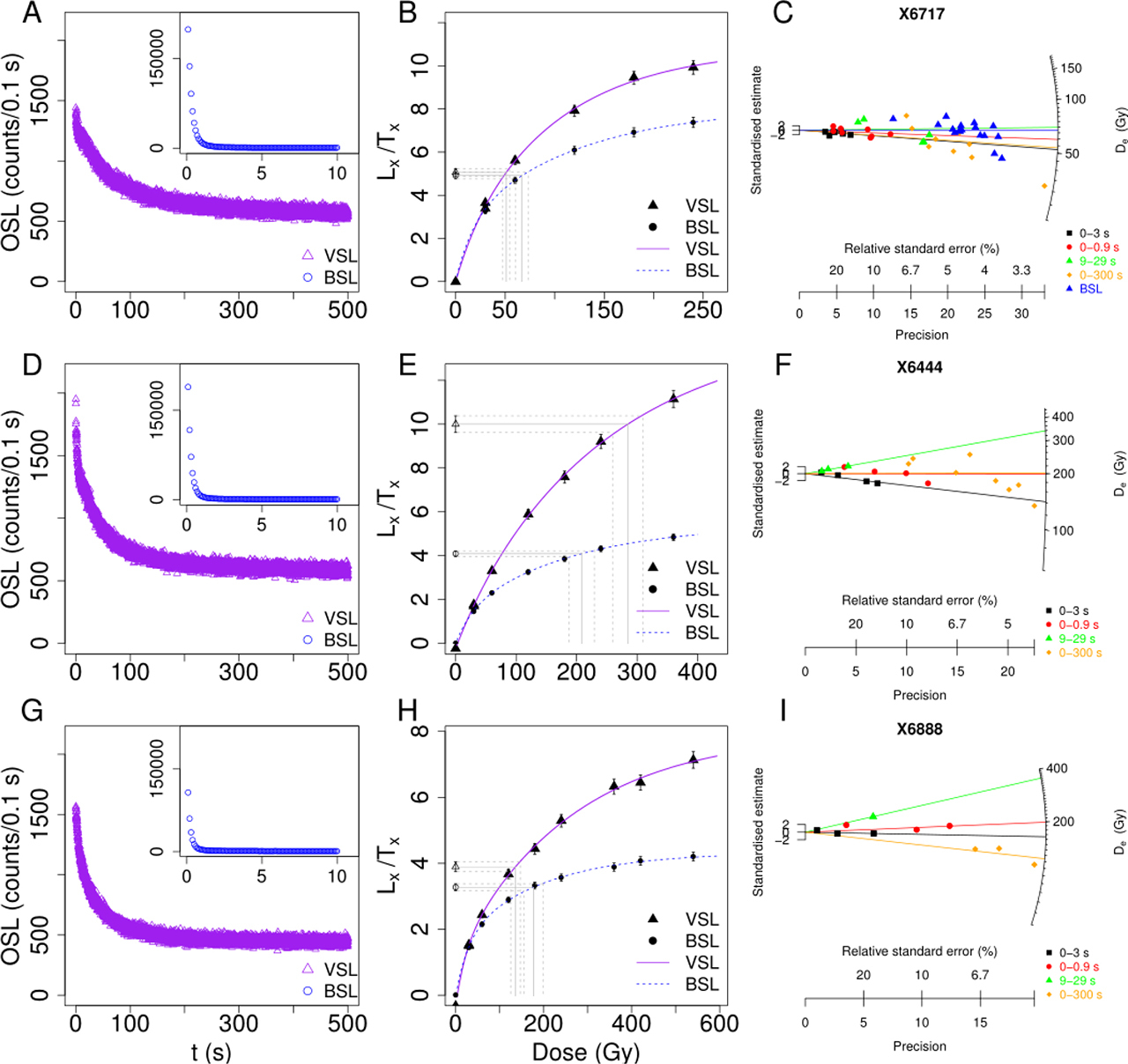
Table 2
Protocols used in this study. Alterations are in bold. Note that for the MAAD protocol, only the measurement parameters were based on Ankjærgaard et al. (2016), not the method to estimate the De.
| Step | SAR (adapted from Hernandez and Mercier (2015)) | MAAD (adapted from Ankjærgaard et al. (2016)) | Function |
|---|---|---|---|
| 0 | - | Additive dose | |
| 1 | Preheat (260°C, 10 s) | Preheat (300°C, 100 s or 10 s) | Empty thermally unstable components |
| 2 | Blue bleach (125°C, 40 s) | Blue bleach (125°C, 100 s) | Empty shallow trapped charge |
| 3 | VSL (125°C, 500 s) | VSL (30°C, 500 s) | Measure deep trapped charge (Ln, Lx or La) |
| 4 | Violet bleach (200°C, 500 s) | - | Reduce recuperation |
| 5 | Test dose (18 Gy) | Test dose (50 Gy) | Sensitivity correction |
| 6 | Preheat (260°C, 10 s) | Preheat (300°C, 100 s or 10 s) | Empty thermally unstable components |
| 7 | Blue bleach (125°C, 40 s) | Blue bleach (125°C, 100 s) | Empty shallow trapped charge |
| 8 | VSL (125°C, 500 s) | VSL (30°C, 500 s) | Measure deep trapped charge (Tn, Tx or Ta) |
| 9 | Violet bleach (200°C, 500 s) | - | Reduce recuperation |
| 10 | Regenerative dose | - |
Dose-response curves were built for samples X6717, X6444 and X6888. The VSL signal was integrated over the first 300 s signal interval and taking the 400–500 s interval as background, while the BSL signal was integrated using the first 0.09 s of signal and the last 10 s as background. Fig. 1B, 1E, 1H show the VSL and BSL growth of the sensitivity-corrected signal (Lx/Tx) of representative aliquots for the three samples fitted with a double saturation exponential function. Equivalent dose (De) values were obtained by interpolation of Ln/Tn onto this function (Duller, 2015; Peng et al., 2013). Between three and thirteen aliquots of each sample were analysed in this manner, though a few were fitted with an exponential plus linear function.
It has been reported that variation of the VSL signal integration limits affects the De estimate, because of the contribution from different components. Ankjærgaard et al. (2013) defined two components, A and B (0–3 and 9–29 s, respectively), using an early-background approach (3–10 and 29–80 s, respectively). A longer signal interval (0–300 s, 400–500 s BG) has been suggested by Hernandez and Mercier (2015) to account for differences in decay shape. To investigate the effect of integration limits, De values were determined using the three integration intervals mentioned above and a late-background fast interval (0–0.09 s; 450–500 s BG) (Fig. 1C, 1F, 1I). Average De values were calculated using the central age model (CAM) (Burow, 2017; Galbraith et al., 1999). Aliquots were accepted if the following criteria were met: natural test dose signal (Tn) at least 3σ above the corresponding background and with a relative error under 25%, negligible recuperation (<5%) and recycling ratio consistent with unity (1.0 ± 0.1). The laser power used in this study was similar to that in Ankjærgaard et al. (2013), so we have maintained the original interval lengths, though it should be noted that our decays are expected to occur ∼20% faster. The laser power used by Hernandez and Mercier (2015) was almost 4x higher than in the present study; however, we used the same integration limit of 0–300 s, seen as the aim of this interval is not to capture a single component, but rather to capture any changes in decay curve shape by integrating over a long decay time.
Use of the different intervals resulted in a variation in CAM De values and in the number of accepted aliquots (Table 3). For the youngest sample (X6717), the component B interval (9–29 s) CAM De of 69.8 ± 11.8 Gy best agreed with the expected result of 67.3 ± 3.0 Gy. For the two older samples (X6444 and X6888), the determined De were mostly below the expected dose, except for that of component B (9–29 s) for X6444, 339.9 ± 67.4 Gy, expected to be >300 Gy. The other intervals for X6444 delivered De below the minimum expected dose by 25–50%. The CAM De values of X6888 underestimated the expected dose range of 600–1190 Gy for this sample by 60–75%, depending on the signal interval used. For all samples, component B resulted in the highest dose equivalents. It is noteworthy that component B has previously been considered unsuitable for dating due to high recuperation rates up to ∼20% (Morthekai et al., 2015) and larger underestimations than component A (Ankjærgaard et al., 2013).
Table 3
VSL De estimates using the SAR protocol. The VSL De values that match the expected dose at 1 sigma are in bold type.
| Sample | Signal (s) | Background (s) | #1 | Overdispersion (%) | De ± se (Gy)2 |
|---|---|---|---|---|---|
| X6717 | 0–0.9 | 450–500 | 8/12 | 13.3 ± 6.5 | 59.7 ± 4.1 |
| 0–300 | 400–500 | 10/12 | 32.1 ± 7.4 | 53.6 ± 5.5 | |
| 0–3 | 3–10.5 | 7/12 | - | 52.4 ± 3.9 | |
| 9–29 | 29–80 | 5/12 | 36.7 ± 12.3 | 69.8 ± 11.8 | |
| X6444 | 0–0.9 | 450–500 | 4/13 | 14.7 ± 8.9 | 199.4 ± 19.8 |
| 0–300 | 400–500 | 8/13 | 27.2 ± 7.2 | 202.2 ± 20.1 | |
| 0–3 | 3–10.5 | 4/13 | - | 141.5 ± 14.1 | |
| 9–29 | 29–80 | 3/13 | - | 339.9 ± 67.4 | |
| X6888 | 0–0.9 | 450–500 | 3/3 | - | 199.0 ± 12.4 |
| 0–300 | 400–500 | 3/3 | 5.5 ± 4.8 | 124.7 ± 5.8 | |
| 0–3 | 3–10.5 | 3/3 | - | 165.2 ± 25.2 | |
| 9–29 | 29–80 | 1/3 | - | 354.5 ± 61.0 | |
It is also of note that for all samples the VSL growth curve saturates earlier than expected, with 2D0 values in the range 350–600 Gy. This is in sharp contrast to the dose-response reported previously (Ankjærgaard et al., 2013, 2016), where the VSL signal has been shown to saturate at doses over 2000 Gy. This indicates that the targeted late-saturating VSL signal was not well isolated for our samples with this protocol.
. MAAD PROTOCOL
Ankjærgaard et al. (2016) reported a difference in shape between the natural and the subsequent regenerative dose VSL decay curves, which can induce discrepancy in the De estimates. These authors suggested the use of a MAAD protocol in order to circumvent this issue. Here, we applied a post-blue VSL MAAD protocol following the parameters in Ankjærgaard et al. (2016), where the VSL signal is detected after a high temperature preheat of 300°C for 100 s. In initial measurements, we observed a significant depletion of the VSL signal (Fig. 2A, orange triangles). Therefore, we shortened the preheat length to 10 s. Details of the protocol are reported in Table 2. Series of three and six aliquots were used for each dose point of sample X6444 (0, 100, 200, 400 Gy) and X6889 (0, 50, 100, 200, 400 Gy), respectively. Aliquots were accepted if the natural test dose signal (Tn) was at least 3σ above the corresponding background and had a relative error under 25%. Outliers were rejected if the normalised median absolute deviation (nMAD) of log La/Ta of each dose point was greater than 2.5 (using 1.4826 as the correction factor for a normal distribution) (Powell et al., 2002, Clarkson et al., 2017) and from the accepted data a CAM was calculated for each dose point (Galbraith et al., 1999). De values were obtained using a classical MAAD approach (Aitken, 1998) by extrapolating the growth curve fitted to the CAM values to 0 dose, since no modern samples were collected at the selected sites.
Fig. 2
MAAD protocol results for samples X6444 (A–C) and X6889 (D–E). (A,D) show the natural dose decay curves and (B,C,E) show the dose response using the signal interval 0–300 s (BG: 400–500s). (B,E) resulted from the shortened preheat (10 s) measurement (purple triangles in (A,D)), while (C) resulted from the 100 s preheat measurement (orange triangle in (A)). The CAM of nMAD accepted aliquots were fitted with a linear function in (C) and an exponential function in (E). The green vertical lines correspond to the expected De. Error bars show the standard errors.
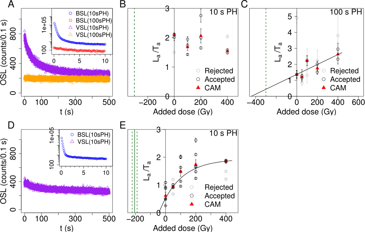
Fig. 2 shows the MAAD results of samples X6444 and X6889. The VSL decays (Fig. 2A, 2D) are similar to those described for the SAR protocol, though the signals are dimmer in this case. An increase of 40°C in preheat temperature (equal lengths of 10 s) led to a 60% initial signal decrease for sample X6444 (cf. Fig. 1D and Fig. 2A, purple triangles), whereas an increase from 10 to 100 s preheat length (equal temperatures of 300°C) almost fully depleted the signal of this sample (cf. Fig. 2A purple and orange triangles). Furthermore, the short pre-heat of 10 s already significantly depleted the signal of sample X6889 (Fig. 2D).
Three different integration intervals were tested to construct a DRC: 0–300 s with a late background, 0–3 s with an early background, and 9–29 s with an early background, with the latter two corresponding to components A and B of Ankjærgaard et al. (2013), respectively. None of the three intervals tested for sample X6444 using the shorter preheat length (10 s) displays a clear signal growth with increasing dose, as shown for the 0–300 s interval in Fig. 2B. Of the three signal intervals tested for sample X6889 using the 10 s preheat length, only the long signal interval (0–300 s) (Fig. 2E) shows a satisfactory dose response. An exponential function was fitted to the CAM of accepted dose points using a Nelder-Mead Simplex algorithm and the absolute value of its intersection with the x-axis, considering its associated uncertainty provides an estimate of the De of 43.6 ± 17.6 Gy. When compared with the expected De of 204.5 ± 16.3 Gy, we observe an underestimation of around 70%. Additionally, this signal component appears to reach saturation earlier than expected for the VSL signal, with a D0 value of 140 Gy added dose (atop 204.5 ± 16.3 Gy natural dose), corresponding to a 2D0 value of ∼690 Gy in this case.
Despite the very low VSL signal decay of sample X6444 using the long preheat of 100 s (see Fig. 2A), integration of the 0–300 s interval displays a signal growth with increasing added dose (Fig. 2C). The best fit of the CAM values was given by a linear function, though the fit is poor, having an adjusted R2 value of 0.57. Extrapolation of the linear function, considering its residual standard error, delivers a De estimate of 442.5 ± 171.3 Gy, which exceeds the minimum expected dose of 300 Gy. Given the poor fit, this result is not deemed significant in terms of age estimation, but the comparison of the signals using the different preheat lengths suggests that the cause of the observed lack of signal growth after the short preheat lies in the dimness of the pB-VSL signal relative to the incompletely bleached slow blue signal.
. DISCUSSION
We tested the applicability of two protocols, namely a SAR protocol (following Hernandez and Mercier (2015)) and a MAAD protocol (following protocol parameters of Ankjærgaard et al. (2016)), to determine the De of sedimentary quartz samples using VSL. For one low-dose sample (X6717), the VSL-SAR De is in agreement with the expected De value of 67.3 ± 3.0 Gy using the component B interval (9–29 s). However, for two higher-dose samples, VSL-SAR resulted in underestimations. The minimum expected De of X6444 was only achieved by component B (9–29 s; 339.9 ± 67.4 Gy), while the other intervals underestimated by up to 50%. All signal intervals of X6888 underestimated the expected minimum De of 600 Gy by 40–80%. This finding is in agreement with previous research on VSL-SAR, which shows agreement with independent age controls for samples below 200 Gy (Ankjærgaard et al., 2015; Porat et al., 2018), but with severe underestimations of up to 80% reported for samples with expected De values of 300–8000 Gy (Ankjærgaard et al., 2015, 2016; Colarossi et al., 2018; Morthekai et al., 2015). For this reason, a MAAD protocol was tested for the higher-dose samples.
The results using the MAAD protocol were more difficult to interpret. Using the short preheat of 10 s, which depletes less of the pB-VSL signal (see Fig. 2A), a De estimation was only possible using a long integration limit for one of the samples (X6889, Fig. 2E), but which underestimated the expected dose of 204.5 ± 16.3 Gy by 70%. It was not possible to build a MAAD growth curve for the other sample (X6444) using this preheat length. The successful growth curve (X6889, Fig. 2E) suggests the onset of saturation of the VSL signal already at 700 Gy using the short-preheat MAAD protocol (2D0 value of 690 Gy). This is higher than the saturation observed for the SAR protocol (2D0 range: 350–600 Gy), which had shorter BSL bleach lengths and lower temperature preheats. While the observed MAAD saturation dose would be an improvement relative to conventional BSL dating, it is much lower than the expected value for the VSL signal, which has been shown to grow up to at least 1800 Gy (Ankjærgaard et al., 2016), indicating that the high-dose saturating VSL signal was not successfully isolated in our protocol. This is presumably caused by insufficient bleaching of the slow-blue component. In contrast, using the original 100 s preheat length allowed for a DRC to be constructed, despite the very dim signal. For either preheat lengths, only the long signal integration interval (0–300 s) resulted in growth curves, presumably because the large uncertainty caused by the low signal levels is counterbalanced by the long average.
The signal decay of X6444 using the short preheat (Fig. 2A) appears to be dominated by the incompletely bleached slow blue component. One of the slow blue components (S2 in Singarayer and Bailey (2003) and S3 in Jain et al., 2003) has been shown to saturate early at 150 Gy (Singarayer and Bailey, 2003), which would explain why we do not observe any signal growth after adding dose atop the natural dose of at least 300 Gy. The early saturation of X6889 can also be explained by an incompletely bleached slow blue component, given that the VSL signal is so dim that any small residual slow blue would contribute to the signal. Other multiple aliquot approaches may be able to elucidate this issue. For example, in the MAAD protocol of Ankjærgaard et al. (2016), the DRC was built using younger samples from the same site, allowing the DRC to be established for low doses even when dating high dose samples. In this case, early signal saturation would be clearly identifiable.
The poor bleaching of the slow blue component in both the SAR and MAAD protocols is probably caused by inappropriate preheating and/or BSL bleach length. Previously, it has been shown that preheat stringency must be balanced between minimizing the slow blue component without excessively depleting the VSL signal. For example, Porat et al. (2018) report a doubling of the D0 value with a 10°C preheat/cutheat increase, but with severe signal depletion. Our results show a similar trend: regardless of signal interval, the MAAD results do not display the expected late-saturating dose response unless the preheat stringency is increased to the point of almost fully depleting the pB-VSL signal, which then leads to large uncertainty. Thus, it seems likely that the pB-VSL of samples X6444 and X6889 are too dim relative to the slow blue component to be measurable with the present experimental set-up.
More work is needed to optimise protocol parameters that isolate the late-saturating pB-VSL, for which brighter samples should be chosen. It must also be investigated what the relationship between the slow blue component and the pB-VSL signal is and whether there is a correlation in the brightness of the components. Our results using the long preheat indicate that it may be possible to date dim samples for which almost no signal decay is observed, but that a much larger number of aliquots would be needed to statistically counter the large scatter caused by the low signal brightness.
. CONCLUSION
Our findings indicate the need for further refinement of the VSL protocol to make it suitable to date natural high-dose samples. In particular, the sufficient bleaching of the slow blue component without depletion of the pBVSL signal seems to be problematic. The behaviour of VSL also appears to be sample-dependent, which may make it challenging to establish a broadly-applicable protocol.