Numerical Modeling of Microbial Fate and Transport in Natural Waters: Review and Implications for Normal and Extreme Storm Events


Department of Civil and Environmental Engineering, Michigan State University, East Lansing, MI 48824, USA
*
Authors to whom correspondence should be addressed.
Water 2020, 12(7), 1876; https://doi.org/10.3390/w12071876
Submission received: 6 June 2020
/
Revised: 24 June 2020
/
Accepted: 27 June 2020
/
Published: 30 June 2020
(This article belongs to the Special Issue Modelling Microbial Water Quality and Health Risk)
Abstract
:Degradation of water quality in recreational areas can be a substantial public health concern. Models can help beach managers make contemporaneous decisions to protect public health at recreational areas, via the use of microbial fate and transport simulation. Approaches to modeling microbial fate and transport vary widely in response to local hydrometeorological contexts, but many parameterizations include terms for base mortality, solar inactivation, and sedimentation of microbial contaminants. Models using these parameterizations can predict up to 87% of variation in observed microbial concentrations in nearshore water, with root mean squared errors ranging from 0.41 to 5.37 log10 Colony Forming Units (CFU) 100 mL−1. This indicates that some models predict microbial fate and transport more reliably than others and that there remains room for model improvement across the board. Model refinement will be integral to microbial fate and transport simulation in the face of less readily observable processes affecting water quality in nearshore areas. Management of contamination phenomena such as the release of storm-associated river plumes and the exchange of contaminants between water and sand at the beach can benefit greatly from optimized fate and transport modeling in the absence of directly observable data.
1. Introduction
Water systems and the recreational opportunities that they afford bring millions of people outside each year, especially during warm weather. Over 75% of people traveling in the summer visit beaches, and in Chicago alone 20 million people go to Lake Michigan beaches annually, on average [1,2]. To protect public health and the safety of beachgoers, the Beaches Environmental Assessment and Coastal Health (BEACH) Act of 2000 requires routine monitoring of coastal water quality at both marine and freshwater beaches across the USA [3]. This monitoring, however, often involves obtaining samples and either culturing for fecal indicator organisms (FIO) such as E. coli or enterococci or using quantitative Polymerase Chain Reactions (qPCR) to determine FIO concentrations in the water. These approaches take time, leading to a delay of up to 24 hours before obtaining water quality information to effectively manage beach usage for public health. This delay can be the difference between keeping beachgoers safe by advising against beach access and putting them in danger by keeping a contaminated beach open for recreation.
To avoid the lag time associated with water sample analyses, mechanistic, statistical and other data-based models have emerged as potentially feasible alternatives to daily water quality monitoring. These models incorporate parameters associated with meteorology, hydrodynamics, human and wildlife usage, water turbidity, and settling of suspended sediments to predict microbial concentrations [4,5,6,7,8,9,10,11,12,13,14,15,16,17,18,19,20].
Numerical mechanistic models have shown variable success in predicting microbial concentrations in coastal and beach systems across space and time. As knowledge of aquatic systems and their various influences on waterborne microorganisms has progressed in recent years, predictive capacity of models has increased as well [13,16,17,21]. However, with a still incomplete knowledge of how components of the aquatic environment interact to influence microbial fate and transport, improving the representation of processes as well as of source behavior, parameter identification and model evaluation remains an evolving process.
This process is further complicated by the often rapidly changing conditions within aquatic environments. For example, Lakes Michigan and Huron in the Laurentian Great Lakes, USA, have become significantly clearer since the 1990’s, in response to an invasion by dreissenid mussels [22,23,24]. This clarification likely impacts microbial survival in the water, due to the subsequent changes in sunlight extinction and solar microbial inactivation rates in the water [25]. Similarly, changes to microbial sources and hydrodynamics associated with climate change [26,27,28,29] may lead to changes in how microbial fate and transport can be effectively modeled. Not only is sea level predicted to rise due to climate change, but frequency and intensity of storm events are projected to increase for many regions as well [30]. Sea level rise will undoubtedly change the layout of beach areas, leading to phenomena such as shoreline erosion and increased foreshore areas that are susceptible to microbial transfer between water and sand [31]. At the same time, a predicted increase in the frequency and intensity of storm events will likely lead to increased runoff of urban and agricultural contaminants to rivers, which will in turn flow to coastal areas and potentially impact beach water quality [32].
Herein, we aim to compare the various approaches to modeling microbial (i.e., FIO) fate and transport in coastal aquatic environments using coupled mechanistic hydrodynamic and transport modeling approaches, to determine how these approaches impact model predictive capability. Examples of such models include the Finite Volume Community Ocean Model (FVCOM, [33]), the Princeton Ocean Model (POM, [15,20,34,35]), the Aquatic Ecosystem Model 3D (AEM3D, [17]), Delft3D [36], and the Environmental Fluid Dynamics Code (EFDC, [37]) to name only a few. For the purposes of this review, we will concentrate on these mechanistic and process-based models of FIO fate and transport, but statistical and data-based modeling approaches are briefly discussed to the extent that they can support mechanistic modeling efforts. We then discuss the application of such approaches to emerging modeling questions surrounding the simulation of storm-associated river plumes and microbial exchange between beach sand and water. While nearshore environments harbor a variety of microorganisms, including bacteria, viruses and fungi, this work will focus on modeling of FIO such as E. coli, enterococci, and coliforms. Understanding how numerical models predict water quality will lend insight into which approaches may be most appropriate for modeling recreational water quality to ensure public health in the face of climatic and environmental changes.
2. Modeling Hydrodynamics and Microbial Fate & Transport
Numerical modeling of hydrodynamics in coastal environments depends heavily on the physics of the water body, meteorological conditions over time and the impacts of river/estuary inputs. Water moves in three spatial dimensions and over time, so utilizing a three-dimensional hydrodynamic model is key to adequately simulating water movementin coastal areas. Unstructured grid models (e.g., FVCOM) may have advantages in simulating coastal water quality due to their ability to accurately represent nearshore features such as irregular coastlines, barrier islands and sandbars, harbors, breakwaters etc.
Generally, coastal hydrodynamics are governed by three-dimensional, unsteady forms of the Navier-Stokes momentum equations (Equations (1)–(3)) and the assumption of the continuity equation (Equation (4)) [33,38,39].
In these equations, x, y, and z represent the east, north and vertical directions, while u, v, and w denote the velocity components in the x, y, and z directions, respectively (m s−1). fu, fv are the Coriolis terms, Fu, Fv are the horizontal diffusion terms in the x and y directions, respectively and Fw is a vertical diffusion term (m2 s−1). Km denotes a vertical eddy viscosity coefficient (m2 s−1) and represents the density of water (kg m−3). Air pressure at the water surface is denoted by pa, hydrostatic pressure is represented by pH, and q is the non-hydrostatic pressure (all in Pa) [33]. Using these equations, models can effectively account for the effects of temperature, density, and Coriolis force on water movement over time. The effects of waves in the nearshore environment (e.g., wave-current interactions, bottom shear stress) can be simulated using coupled hydrodynamic and spectral wave models such as the FVCOM-Surface Wave (FVCOM-SWAVE) model [40].
Building on the general hydrodynamic model, microbial fate and transport associated with diffusion, dispersion, advection, and mortality within an aquatic system can be simulated [9,12,13,15,16,17,20,21,41]. The governing equation for microbial fate and transport is based on the advection-dispersion-reaction (ADR) equation, formulated in terms of FIO concentration (Equation (5)). This equation includes terms for advection, diffusion/dispersion in the water column, and microbial decay [16,33].
In the equation, C corresponds to the microbial concentration (Colony Forming Units (CFU) 100 mL−1), k represents the overall microbial decay rate (d−1), and KV and KH are the vertical and horizontal mixing coefficients, respectively (m2 s−1). Horizontal and vertical mixing are described using the Smagorinsky and Mellor-Yamada 2.5 level turbulence parameterizations [33,39]. Microbial decay can depend on factors such as microbial taxon and base mortality, water temperature and chemistry, attachment to and detachment from suspended solids, settling after attachment to suspended solids, sunlight inactivation, and interactions with other biota in the aquatic environment [21]. Because of its dependence on these factors, the decay term in mechanistic models has taken on many forms within the literature and is often a combination of multiple terms.
3. Boundary and Initial Conditions
Key drivers of hydrodynamics in the nearshore region include winds and/or tides [42,43] and riverine/estuarine flows [9,44,45,46]. These are often governed by local conditions such as bathymetry, wind stress, Coriolis force, and water temperature, which can vary spatiotemporally. For example, seasonality of thermal or density stratification in large lakes such as Lake Michigan can impact circulation as well as buoyancy of contaminant plumes, leading to differential impacts on water quality and hydrodynamics throughout the year [47,48]. Similarly, estuarine exchange flows and the corresponding changes in vertical density stratification (and hence vertical mixing) are controlled by the along-channel wind component which changes seasonally [49]. In addition to seasonal-temporal variability in fluid properties, there are spatial influences that control hydrodynamics. The impacts of Coriolis force can vary by latitude as well as water body size, with effects becoming significant for large (>5 km width) lakes and at high latitudes [50]. Because these effects can vary spatiotemporally while also influencing large-scale hydrodynamics by influencing stratification, it is important to specify related model boundary conditions as realistically as possible.
Boundary conditions for the momentum equations are well-known and include wind stress on the surface of the water column and bed friction on the lake/seabed; additional details are available in Chen et al. [33,39]. For the FIO transport model, the nature of the source(s) dictates the type of boundary conditions used. For beaches impacted by riverine sources, monitoring data collected at the river mouth can be used to provide boundary forcing for the FIO transport model. However, most mechanistic models use small time steps (on the order of seconds to minutes) while monitoring data are collected less frequently (e.g., weekly or bi-weekly), introducing significant uncertainty into the modeling due to a mismatch between the model time steps and forcing data. In addition, model inputs are generally specified at regular intervals while monitoring data may be irregular and with gaps (e.g., missing data during weekends).
One way to address this limitation is to use calibrated watershed models [51,52,53] or statistical models to generate high-resolution boundary forcing data at the river mouth when high-resolution discharge data are available (e.g., at a United States Geological Survey (USGS) gauging station in the USA). Several researchers have exploited a potential correlation between river discharge (Q) and FIO (e.g., E. coli) concentrations (C) and have used statistical relations between Q and C to generate high-resolution tributary loading data for nearshore FIO models [16,17,20]. Compared to the use of sparse monitoring data to represent tributary loading in FIO models, these approaches have promise, as they can better describe rapid changes in loading and may be suitable for simulating the impacts of extreme storm events on microbial water quality in coastal areas. For beaches with no known riverine sources, observed FIO dynamics may be driven by local sources including birds [12,54,55], resuspension of bottom sediment-bound FIO [45,46] and shoreline sand [7,56]. A comprehensive analysis of the relative importance of the different sources calls for detailed modeling of hydrodynamics including currents and waves, sediment transport, sediment-FIO interactions and relatively fine computational grids to capture the impact of shoreline birds and sand. Because initial conditions for hydrodynamic models of lakes and reservoirs may specify a waterbody that is initially at rest (zero velocity components), a spin-up period is often used to allow models to catch up with observed data. For FIO models, the initial concentration of FIO may include a small non-zero background value and model spin-up time may allow for increased water quality predictability over the model simulation period.
4. Components of the Microbial Decay Function
One form of the microbial decay function from Equation (5) is represented by Equation (6), where total microbial loss (k) is characterized by the combination of a base mortality rate (kb1), light inactivation rate (kbi) and settling rate (kbs) [41,57]. All of the decay terms in the equation are daily decay rates (units of d−1).
The factors that influence these three terms, though, can be variable and specific to the model domain, context, and aims.
Liu et al. [13] further separated this basic decay function for Lake Michigan, yielding a function that accounted for bacterial loss due to settling and light inactivation, with a temperature correction factor to justify changes due to temperature variations from 20 °C (Equation (7)). In this model, fp is the fraction of FIO particles attached to suspended solids (unitless), vs represents settling velocity (m d−1), H is the depth of the water column (m), kI is the inactivation rate associated with solar radiation (m2 W−1 d−1), It denotes the solar irradiance at the surface of the water at time t (W m−2), θ is the temperature correction factor (unitless), and T is the water temperature (°C).
The right-hand side of this equation is composed of a sedimentation/settling term, a light inactivation term, and a temperature correction factor, when read from left to right. Though it incorporates terms for temperature, settling, and sunlight impacts on FIO, this form of the decay function fails to account for other potentially important influences.
Microbial survival in aquatic systems can be subject to impacts due to temperature, salinity, light penetration and inactivation, predation, competition for resources, nutrient availability, and other natural (or base) mortality. Similarly, conditions such as the presence of aquatic vegetation and dreissenid mussels in a water body can impact bottom shear stress, thereby influencing sedimentation and resuspension of FIO. These factors can be difficult to characterize, especially when they vary between systems. In marine or brackish ecosystems where salinity may vary over time and space, it can have a substantial impact on the survival and persistence of several microorganisms [21,58,59,60,61,62,63,64,65,66]. Similarly, in systems with high levels of mixing or turbidity, FIO may not settle out of the water column as much as they would for less well-mixed systems that would foster settling [67]. Finally, light inactivation has been shown to play a significant role in FIO decay via inactivation in natural waters [68,69]. This is especially true for oligotrophic or low-turbidity waters that do not have high levels of suspended solids that can serve as refugia for FIO [25].
Impacts can also vary between different microorganisms. Cabelli [70], Colford et al. [71], and Schang et al. [72] document differential sensitivities to environmental pressures between E. coli, Cryptosporidium parvum, Giardia lamblia, and Campylobacter spp. in natural waters. Sanders et al. [73] tested the impact of organism-dependent sensitivities to environmental survival influences on model predictive ability. They found that a model with the same environmental influences underpredicted E. coli concentrations, but overpredicted concentrations of both total coliforms and enterococci, compared to observations.
4.1. Dark Mortality, Base Mortality and Temperature/Salinity Dependence
Base mortality (kb1) and dark mortality (kd) terms are often used in models to account for the natural decay that microbes undergo, independent of sunlight effects. The value of kd can be highly variable, depending on the geographic location and the microorganism of focus [15,16,21,74,75,76,77]. Models have been presented using kd values as low as 8.6 × 10⁻⁵ d−1 [15] and in vitro experiments have yielded kd rates of up to 2.2 d−1 [74]. Once kd is established, it is then possible to correct for other factors affecting kb1, such as temperature, salinity, or pH of the water.
While salinity and its impacts on microbial persistence are frequently negligible in freshwater systems, marine and estuarine systems often have dynamic salinity conditions, and microbial decay rates are proportional to salinity levels [21,58,59,60,61,62,63,64,65,66]. As a result, models in the context of marine or estuarine systems calculate kb1 in terms of salinity, using either percentage of sea water (Ps, [59]) or salinity (S, PSU) terms (Equations (8) and (9)).
Dark mortality rates are developed for a reference water temperature of 20 °C, so an adjustment to account for variability in temperature is also needed. Microorganism base mortality terms are adjusted for temperature using the Arrhenius equation [15,18,78]. Resulting temperature correction factor values can range from 1.04 to 1.11 [78], but frequently are assumed to be 1.07 [79]. This adjustment indicates a strong temperature dependence, with a doubling of the mortality rate for every 10 °C increase in temperature [41]. The resulting full formulation of the base mortality term is thus represented by equations 10 and 11, where θ represents the temperature correction factor.
A majority of existing models use some version of this formulation to determine base mortality rate of microorganisms in natural waters (Table 1). Notable exceptions were found in models from Liu et al. [80], McCorquodale et al. [81], Hipsey et al. [21], Rehmann and Soupir [78], Servais et al. [82,83], and de Brauwere et al. [84]. Rather than using a dark mortality rate to calculate base mortality, Liu et al. [80] use the time to inactivate 90% of microorganisms in the dark (t90). McCorquodale et al. [81] use a curve-fitting procedure on field-collected data to determine the impact of salinity on base mortality. Hipsey et al. [21] and Rehmann and Soupir [78] incorporate the effects of salinity and pH on mortality ( and , respectively), sensitivity of the microorganism to salinity and pH (β and , respectively), nutrient limitation (fLIM) and dissolved organic carbon concentration (DOCL) when calculating base mortality. Following Servais et al. [82,83], de Brauwere et al. [84] use a logistic relationship between microbial decay and temperature to determine kb1.
4.2. Solar Inactivation Terms
It is generally accepted that incoming solar radiation affects the survival of microbes in water systems [69,85,92,93]. This is especially true in clear, oligotrophic waters, where solar inactivation can be a predominant influence on microbial survival [25,68]. Many mechanistic fate and transport modelers recognize the impacts of solar inactivation on microbial survival in water and include inactivation parameters in their models.
Accounting for solar irradiation in natural waters inherently involves the calculation of the light extinction rate within the water column. The amount of light penetrating the water column declines exponentially with depth and is influenced by the turbidity or clarity of the water, such that clearer water yields a lower light extinction rate than turbid water. Lower light extinction rates, in turn, yield more intense solar radiation at deeper depths in the water, leading to higher microbial solar inactivation rates [41].
Nearly all of the models which account for solar inactivation use some variation of Equation (7) in which the Beer-Lambert Law (Equation (12), [94]) is used to model the variation of solar radiation with depth. In the Beer-Lambert equation, z is vertical coordinate of depth (m) and Iz represents the amount of solar radiation at vertical coordinate z (W m−2). I0 is solar radiation at the water surface (W m−2), and ke is the light extinction rate (m−1) [95]. It is important to distinguish between kI from Equation (7) and ke in Equation (12). In Equation (7), the kI term is an inactivation rate for FIO as a result of solar radiation [16,73,80], whereas ke in Equation (12) is the rate of light extinction with depth in the water column [21,41,95].
Model type can have a significant impact on the variables used in parameterization of solar inactivation effects on FIO. Models may employ either total depth (H) or the vertical coordinate (z) within their solar radiation parameterizations, depending on the model context. In two-dimensional model frameworks, conditions within the water column are often vertically-integrated. For these cases, fate and transport models use a single depth variable (H) and a single solar radiation variable (It) to account for potential variability in the vertical dimension [13,41,45,78]. Fully three-dimensional models, in contrast, explicitly define conditions at different depths in the water column via their incorporation of the vertical coordinate variable z within their parameters. For example, fully three-dimensional models will often incorporate variables for solar radiation at the water surface (I0) and solar radiation at depth z (Iz) to capture differences with depth in the water column [15,16,21,35,59,74,85,86,90,91,96].
A variety of approaches have been used for characterizing the effects of solar inactivation on FIO fate and transport. In some cases, models do not include solar inactivation terms at all [17,51,76,77,84,88], often because the water is so turbid that solar effects are assumed negligible compared to other environmental influences. Others use either a microbial decay rate solely as a function of incoming solar radiation (Equation (7)) or as a function of the light extinction rate and depth in the water (Equation (12), Table 2). Hipsey et al. [21] expanded the description of solar inactivation effects on FIO in their generic modeling framework, including specific terms for dissolved oxygen (DO), pH, salinity (S), and solar bandwidth (b). Garcia-Alba et al. [18] included terms corresponding to day length (DL) and fraction of solar irradiance that is in the UV spectrum (fUV) as well as the typical light extinction rate, solar inactivation rate, solar irradiance and depth terms seen in other models.
4.3. Sedimentation Terms
In addition to solar inactivation, attachment to suspended solids and settling out of the water column is another significant driver of FIO losses in aquatic environments. 80–100% of total coliforms and E. coli have been shown to readily attach to suspended particles in the water column [100], and viruses have also been shown to easily attach to particulate matter and settle out of suspension [101].
Similar to the solar inactivation term, several published models do not incorporate sedimentation effects on microbial fate and transport [44,73,87,88,90,98,99,102,103]. In models that do incorporate sedimentation losses, settling terms most frequently use parameters representing settling velocity (vs, as calculated using Stokes’ Law), vertical coordinate (z) or the total water column depth (H), and the fraction of the FIO that is attached to particles (fp, Table 3). In many cases, sedimentation terms are also subject to temperature correction, in the same manner that base mortality and solar inactivation terms utilize temperature correction factors [13,16,76,77], to acknowledge the fact that overall loss of FIO increases with temperature.
In their generalized sedimentation term, Hipsey et al. [21] expanded upon the simplified sedimentation terms used in most other models. This expansion accounts for various particle size classes (Ns), particle and attachment surface areas (Ap and As, respectively), and settling velocities for attached (vs) and unattached (vc) FIO.
Bravo et al. [20] and Thupaki et al. [35] incorporated sedimentation effects by including them in the vertical advection term of the 3D ADR equation (Equation (5)). As a result, the ADR presented is Equation (13) and the microbial decay function (kC) only includes terms for base mortality and solar inactivation in these models.
5. Model Testing and Evaluation
There is a large number of processes influencing FIO fate and transport and it can be difficult to identify a correct conceptual model that acknowledges process interdependencies over wide ranges of environmental variables of interest. Therefore, it is difficult to fully test FIO models across environments, and within the same environment, across different time periods (e.g., dry vs. wet weather events, “normal” vs. extreme events). While calibrated FIO fate and transport models have the potential to aid management by providing near real-time predictions, a majority of the published papers report results of model back-testing (or history matching, see Bredehoeft and Konikow [104]).
To evaluate the goodness of fit between models and observational data as well as to identify superior model formulations (by comparing different models), the use of multiple model evaluation metrics may be more beneficial [104,105] than the use of a single metric such as the coefficient of determination (R2) or root mean squared error (RMSE). This is due to the fact that no single model performance metric captures all aspects of the data and simulation results, and all metrics have known limitations. In the context of FIO and beach management, evaluating models using the confusion matrix and concepts of sensitivity and specificity [19,106,107] have proven to be useful, especially for the practical application of issuing beach advisories and closings.
Existing, published models have been tested in a number of ways. Most model testing protocols, particularly those in more recent modeling studies, involve statistical analysis of comparability of model results to observed data. A majority of published models have used RMSE or R2 as model performance metrics (Table 4). Other statistics such as Normalized RMSE (NRMSE), Mean Absolute Error (MAE), Nash-Sutcliffe Efficiency (NSE) [108], Percent Bias (PBIAS) [109] or the Refined Willmott Index of Agreement [110] have also been used by Boye et al. [90], Liu et al. [77] and Feng et al. [98]. A subset of the published models was qualitatively assessed, often with comparisons to other models replacing the more quantitative RMSE, R2, MAE, NSE and Wilmott index statistics [21,38,59,76,78,84,85,87,88]. In all applicable cases, the RMSE or MAE values have units of log10 FIO CFU 100 mL−1, while NRMSE units are percentages and NSE values are unitless.
Based on R2 to evaluate model performance, the model of Garcia-Alba et al. [18] produced one of the best descriptions of observed data among the models considered here (R2 = 0.87). Their model incorporated temperature- and salinity-dependent base mortality () and solar inactivation terms accounting for day length and fraction of irradiance composed of UV radiation (). Based on RMSE alone, one of the published models that best approximates observed microbial concentrations is detailed in Thupaki et al. [15] (RMSE = 0.41 log10 CFU 100 mL−1). Within this model, kb1 = kdθT−20, kbi = (kIIt)·θT−20, and kbs = .
Although comparison of these model frameworks can lend insight into which ones may best simulate microbial water quality, it is important to note that the models were developed under varying contexts. One published approach attempted to develop a generic water quality model, to be used across environments and target microorganisms [21]. This model framework led to complex terms within the decay function, often including parameterization for salinity, pH, dissolved organic carbon concentration, varying particle sizes and settling velocities, and variable sensitivity of the microorganism to such environmental changes. The resulting validation of the model indicated that the generic model did not outperform other existing models in its prediction of contaminant fate and transport. Despite this lack of substantial improvement over existing models, the generality of this model may be attractive to researchers looking for a single model to predict water quality under various conditions.
A lack of ancillary data may provide a confounding factor in the use of generic models such as the one described in Hipsey et al. [21]. In many cases, models are developed without the use of DOC, pH, temperature and salinity data, instead relying on hydrodynamics and meteorology to model FIO fate and transport. Likewise, additional water quality data such as DOC, pH, temperature and salinity are often not collected or available for model development, potentially hindering the usage and applicability of such a generic model. This could, however, indicate not that generic models may be less useful than specific and localized models, but rather that in situ DOC, pH, temperature and salinity data should be collected as part of the water quality monitoring process. For example, while the focus of most FIO modeling efforts is to reproduce the observed FIO concentrations, if no temperature data are collected in the nearshore region the ability of the coupled FIO-temperature-hydrodynamic model to accurately represent FIO decay is questionable as base mortality, solar inactivation, and sedimentation are often functions of temperature. A majority of the models reported in the literature use microbial decay formulations with a solar inactivation term and use FIO data collected during the daytime. Previous research shows that the highest levels of FIO are typically observed during the early morning hours (e.g., 6:00 AM) [111] due to the absence of solar radiation the previous night. Therefore, modeling the nighttime variation of FIO is important to correctly describe FIO levels in the morning [112]; however, since monitoring data are not collected at night, this aspect has not received much attention in the modeling literature.
In the absence of the specific data needed for the generic water quality model described above, selection of an appropriate modeling framework should be based on the target FIO as well as the environmental and hydrological context of the model.
6. Applying Microbial Fate and Transport Models to Extreme Storm Events
Numerical simulation of microbial water quality has evolved in recent years, as the dynamics of processes such as solar inactivation have become clearer. Even so, the incomplete knowledge of influences within aquatic systems on water quality indicates that there is still room for model improvement. Likewise, climate and land use/urbanization changes provide additional contexts for the prediction of microbial water quality [26]. Although the link between extreme precipitation and waterborne disease outbreaks is well known [29,113], the current generation of FIO models can be further refined and tested for their ability to reproduce observed dynamics during extreme storm events. Major areas of research impacting coastal water quality from the perspective of extreme storm events may include the exchange of FIOs between water and sand at beaches, the fate and transport of FIOs in storm-associated river plumes and the expansion of water quality monitoring research into microbial source tracking and environmental DNA (eDNA) for use in public health contexts.
The interaction between water and sand at the beach, and its impacts on recreational safety and water quality, has been an active area of discussion in recent years [56,114,115,116,117,118,119,120]. Microorganisms in beach sands have been cited as potential sources of contamination and swimmer infection as early as 2003 [115]. The microbial community within beach sands is unique [15] in that it can serve as either a sink or a source of FIO to the adjacent recreational water, depending upon wave energies, currents and the movement of the water. When wave energy is low, FIO often get deposited from the water and into shoreline sand where they can form biofilm communities, while higher wave energy frequently leads to the release and re-suspension of FIO from the shoreline sand into the water [56,116]. These sand-based sources and sinks can heavily impact spatial and temporal trends in FIO concentrations at beaches. Further, the Intergovernmental Panel on Climate Change (IPCC) has predicted increases in wind speeds and wave heights/energies in mid- and upper latitudes as a result of climate change [121]. Similarly, the IPCC has predicted sea level rise in coming decades, a phenomenon already being observed, leading to changes in the beach face and the intertidal zone that is impacted by wave deposition/resuspension of FIO [56,122]. This will likely lead to increases in wave-induced FIO release from sands and into recreational water. Because of the potential for climate change to significantly impact sand-water exchange of FIO at beaches, it will be integral for numerical models to include sand-sediment-water interactions when predicting microbial water quality. Currently there are gaps in our understanding of these sand-sediment-FIO related processes and there is a need to further refine our mechanistic modeling approaches based on high-quality field observations and datasets which are often lacking. This will be especially important in substantially wave-impacted beach areas, to improve upon model predictions that exclude sand/sediment parameters [35,46].
Such models accounting for sand-sediment-water interactions at the beach may take inspiration from modeling frameworks that incorporate sedimentation. For instance, the modeling approach developed by Hipsey et al. [21] includes terms for various particle size classes, accounting for differential resuspension effects on “fine” and “coarse” particles. Fine particles require lower bed shear stress values for resuspension, compared to coarse particles, so it may be important to differentiate between the readily resuspended particles and those that are less likely to resuspend after deposition [98,100,123]. After simulating sediment transport as a function of particle size, sediment-FIO interactions can be modeled using attachment-detachment kinetics following those established for subsurface transport models [124].
An additional concern related to how climate change will impact recreational water quality involves storm- and runoff-associated FIO at coastal areas. For many regions, including mid-latitudinal coastal areas, climate change is expected to lead to increasingly frequent and intense storms [121]. Not only will these intense storms make recreation at beaches dangerous via rip tides, rip currents and strong waves, but they will also send increased volumes of potentially contaminated runoff and river water downstream, to be released to coastal areas [125]. As a result, recreational beaches may be expected to experience the impacts of more frequent and larger storm-associated river FIO plumes.
Effective prediction of the coastal water quality impacts from river FIO plumes will be helpful in not only understanding an additional source of contamination to recreational areas but will also aid in the management of beach resources for public and environmental health. This simulation will require the extension of existing numerical modeling approaches to include the determination of FIO concentrations in dynamic river plumes as well as reliable estimation of plume dynamics.
A number of studies have reported a “first-flush” effect for FIO (e.g., [122,123]) in which elevated FIO levels were observed following storm events with levels declining in later portions of the storm event and in subsequent events over a season. However, other researchers did not report such an effect [126]. These differences can be attributed to different runoff characteristics of watershed areas, so linking coastal water quality models with well-tested watershed models of FIO is expected to help address current limitations of nearshore FIO models [127]. For example, microbial composition and concentrations in runoff depend on upstream land uses; runoff from rural/agricultural watersheds is likely to have different water quality concerns than runoff from urbanized or forested catchments [128,129,130]. These differences are magnified during first flush phenomena and heavy storm events, where FIO can be released from soils and into the water, leading to high FIO loads in rivers that can then degrade coastal water quality. Therefore, calibrated upstream watershed models can be beneficial for modeling of coastal water quality in response to storm-associated river plume releases, simply because of the differential impacts resulting from different upstream watershed conditions that send FIO loads downstream to the coast.
In addition to the enteric pathogens of human health concern that can be indicated using FIO, microorganisms that cause other health problems, such as respiratory and skin infections, are also often present at beaches, and may be tracked to upstream sources [131]. This is especially true in the context of extreme storm events when beaches are heavily impacted by upstream river flows and plumes. Methods such as microbial source tracking (MST) and the monitoring of eDNA have shown value in their ability to improve predictive modeling of extreme storm events by offering insights into sources and transport pathways for FIO [7,132]. Differences in MST and eDNA monitoring results between “normal” and heavy storm conditions can be helpful in determining the types of microorganisms that become active within the aquatic environment in response to storm conditions [133]. Similarly, they can be informative in characterizing upstream impacts on coastal areas, by revealing potential catchment sources of microorganisms. Integrating well-calibrated watershed FIO models with nearshore water quality models (e.g., Bedri et al. [53]) or statistical and data-based approaches that describe FIO loading to coastal areas [20] may further improve the performance of nearshore FIO models during extreme events.
Conditions surrounding FIO sedimentation, attachment to suspended solids, and resuspension in riverbeds and coastal areas can vary greatly between storm events. However, there is a notable lack of observational data on water quality during and immediately following different storm conditions. High-resolution FIO data both within and between storm events will be critical to effective simulation of FIO loading, attachment dynamics, sedimentation and resuspension kinetics, and overall water quality in river plumes associated with heavy rain events. It can be difficult to collect these data, due to safety considerations, but the use of sensor networks and small unmanned aerial vehicles has emerged as a potential alternative to field data collection. Morgan et al. [134] demonstrated the use of unmanned aerial vehicles to photograph and document inland irrigation ponds and used image analysis to characterize water quality from the images collected. Many existing sensors on water bodies (e.g., select USGS gauging stations) also collect ancillary water quality data such as turbidity and electrical conductivity. These easy-to-collect data have the potential to help further constrain and evaluate FIO models because of their correlations to microbial water quality [10,11,16,135]. High-resolution water quality data collection is ideal for effective fate and transport modeling, but this data collection can take many forms, including remote sensing and proxy data collection.
In the coastal environment, there are multiple ways to simulate river plumes in numerical water quality models. Along with the river flow inputs, plumes may be characterized by tracking specific FIO within a water quality or FIO-specific model. In these models, FIO concentrations associated with the river inputs and decay function parameters can be specified to reflect local conditions. To assess the relative contributions of FIO from riverine sources to a beach site, constant FIO concentrations or arbitrary FIO masses can be input into the model over a release period [136,137] and breakthrough curves can be generated over time for specific locations. In contrast, FIO concentrations that are associated with riverine flows may be calculated using empirical relationships between river flowrate and FIO concentration [16,17,20]. For beaches impacted by multiple river plumes (e.g., Liu et al. [13]; Kim et al. [138]), the plume dynamics and hence nearshore water quality can be significantly more complex (Figure 1). Using realistic boundary conditions/forcing, models can track the FIO within the plumes spatiotemporally. Another attractive option for simulating FIO plumes involves the use of particle tracking [96,139,140,141,142], especially “reactive” particle tracking models that can account for FIO losses [143]. In this case, FIO are released to the model domain (i.e., river outlets) as discrete particles. Upon their release, the particles’ movements are tracked over time based on the simulated velocity field in three dimensions. This approach, using a Lagrangian formulation for dispersion, has the advantage that it does not suffer from excessive numerical dispersion inherent to Eulerian approaches. All of these approaches have their merits and drawbacks, so it is likely that selection of an optimal framework for plume modeling will require evaluation of the approaches within the context of the research questions and local conditions.
Emerging issues such as water quality degradation associated with FIO exchange between water and sand, river plumes, upstream watershed impacts, and heavy storm runoff are key to effective modeling of microbial fate and transport in coastal areas. As such, future research and modeling in these areas will be beneficial to the water quality modeling community and knowledge base into the future.
7. Conclusions
Numerical models of water quality in nearshore regions can be useful tools for management of recreational water resources. Water quality and FIO fate and transport models within larger coastal ocean modeling frameworks have the potential to predict the fate and transport of FIO and pathogens of human health concern over time and across space. However, these models are only useful if they are refined and validated against observations.
In recent years, development of reliable FIO fate and transport models for aquatic and coastal systems has been an active area of research. As a result, modeling approaches frequently include decay terms associated with base mortality, solar inactivation, and sedimentation, though the specific parameterization of those terms can vary between models [41]. Highly generalized fate and transport models expand upon those terms to account for the effects of salinity, water temperature, pH, dissolved organic carbon, and differential settling rates due to varying particle sizes [21]. Model optimization in terms of FIO tracking has led to frameworks with RMSE values as low as 0.41 log10 FIO CFU 100 mL−1 of water [15]. Some models have also been shown to predict up to 87% of variation in FIO concentrations from observed data [18]. While these validation statistics indicate that model frameworks are improving in their prediction of water quality, there is still room to optimize further. It is also important to note that many of these model parameterizations are specific to their local model domains. Generic models of FIO fate and transport can be developed, but without extensive datasets to test and constrain processes generic model formulations may not offer superior performance compared to simpler models [21]. Therefore, it will likely continue to be imperative that models be developed for their specific contexts, in order to maximize their predictive capacity.
FIO fate and transport modeling frameworks linked to watershed models in the contexts of water-sand exchange at the beach and release of FIO during storms can help us prepare for the potential impacts of extreme events on coastal areas. High quality intra- and inter-event data as well as modeling studies are needed to push the predictive capability of the current generation of FIO models. By refining established FIO decay functions to maximize predictive ability of models and combining those with the diffuse point and non-point FIO sources like plumes and sand-water exchange, prediction and tracking of pollutants in nearshore water and sand can be optimized. Confidence in modeling results can be maximized, allowing for more effective management for public health at nearshore and recreational beach areas in the face of climate and land use change.
Author Contributions
Conceptualization, M.S.P.; Formal Analysis and Investigation, C.J.W.; Writing—Original Draft Preparation, C.J.W., Writing—Review and Editing, M.S.P. and C.J.W., Supervision, M.S.P., Project Administration, M.S.P. All authors have read and agreed to the published version of the manuscript.
Funding
This research was funded by the United States Geological Survey, project number RC108429, titled “Evaluate the Fate and Transport of Historic Backflows from the Chicago Area Waterway System to Lake Michigan”.
Conflicts of Interest
The authors declare no conflict of interest.
References
- Klein, Y.; Osleeb, J.; Viola, M. Tourism-generated earnings in the coastal zone: A regional analysis. J. Coast. Res. 2004, 20, 1080–1088. [Google Scholar] [CrossRef]
- Nevers, M.B.; Whitman, R.L. Efficacy of monitoring and empirical predictive modeling at improving public health protection at Chicago beaches. Water Res. 2011, 45, 1659–1668. [Google Scholar] [CrossRef]
- United States Environmental Protection Agency. 106th United States Congress. In Beaches Environmental Assessment and Coastal Health Act of 2000 (BEACH Act), 2nd ed.; Public Law 106-284. 33 USC 1251; United States Environmental Protection Agency: Washington, DC, USA, 2000; Volume 114. [Google Scholar]
- Nevers, M.B.; Whitman, R.L. Nowcast modeling of Escherichia coli concentrations at multiple urban beaches of southern Lake Michigan. Water Res. 2005, 39, 5250–5260. [Google Scholar] [CrossRef]
- Francy, D.S.; Bertke, E.E.; Darner, R.A. Testing and Refining the Ohio Nowcast at Two Lake Erie Beaches-2008; U. S. Geological Survey: Reston, VA, USA, 2009. [Google Scholar]
- Wong, M.; Kumar, L.; Jenkins, T.M.; Xagoraraki, I.; Phanikumar, M.S.; Rose, J.B. Evaluation of public health risks at recreational beaches in Lake Michigan via detection of enteric viruses and a human-specific bacteriological marker. Water Res. 2009, 43, 1137–1149. [Google Scholar] [CrossRef] [PubMed]
- Nevers, M.; Byappanahalli, M.; Nakatsu, C.; Kinzelman, J.; Phanikumar, M.; Shively, D.; Spoljaric, A. Interaction of bacterial communities and indicators of water quality in shoreline sand, sediment, and water of Lake Michigan. Water Res. 2020, 178. [Google Scholar] [CrossRef] [PubMed]
- Shively, D.A.; Nevers, M.B.; Breitenbach, C.; Phanikumar, M.S.; Przybyla-kelly, K.; Spoljaric, A.M.; Whitman, R.L. Prototypic automated continuous recreational water quality monitoring of nine Chicago beaches. J. Environ. Manag. 2016, 166, 285–293. [Google Scholar] [CrossRef] [PubMed]
- Abu-Bakar, A.; Ahmadian, R.; Falconer, R.A. Modelling the transport and decay processes of microbial tracers in a macro-tidal estuary. Water Res. 2017, 123, 802–824. [Google Scholar] [CrossRef]
- Zhang, Z.; Deng, Z.; Rusch, K.A. Development of predictive models for determining enterococci levels at Gulf Coast beaches. Water Res. 2012, 46, 465–474. [Google Scholar] [CrossRef] [PubMed]
- Zhang, Z.; Deng, Z.; Rusch, K.A.; Walker, N.D. Modeling system for predicting enterococci levels at Holly Beach. Mar. Environ. Res. 2015, 109, 140–147. [Google Scholar] [CrossRef] [PubMed]
- Eregno, F.E.; Tryland, I.; Tjomsland, T.; Kempa, M.; Heistad, A. Hydrodynamic modelling of recreational water quality using Escherichia coli as an indicator of microbial contamination. J. Hydrol. 2018, 561, 179–186. [Google Scholar] [CrossRef]
- Liu, L.; Phanikumar, M.S.; Molloy, S.L.; Whitman, R.L.; Shively, D.A.; Nevers, M.B.; Schwab, D.J.; Rose, J.B. Modeling the transport and inactivation of E. coli and enterococci in the near-shore region of Lake Michigan. Environ. Sci. Technol. 2006, 40, 5022–5028. [Google Scholar] [CrossRef] [PubMed]
- Ge, Z.F.; Whitman, R.L.; Nevers, M.B.; Phanikumar, M.S.; Byappanahalli, M.N. Nearshore hydrodynamics as loading and forcing factors for Escherichia coli contamination at an embayed beach. Limnol. Oceanogr. 2012, 57, 362–381. [Google Scholar] [CrossRef] [Green Version]
- Thupaki, P.; Phanikumar, M.S.; Beletsky, D.; Schwab, D.J.; Nevers, M.B.; Whitman, R.L. Budget analysis of Escherichia coli at a southern Lake Michigan beach. Environ. Sci. Technol. 2010, 44, 1010–1016. [Google Scholar] [CrossRef] [PubMed]
- Safaie, A.; Wendzel, A.; Ge, Z.F.; Nevers, M.B.; Whitman, R.L.; Corsi, S.R.; Phanikumar, M.S. Comparative evaluation of statistical and mechanistic models of Escherichia coli at beaches in southern Lake Michigan. Environ. Sci. Technol. 2016, 50, 2442–2449. [Google Scholar] [CrossRef]
- Madani, M.; Seth, R.; Leon, L.F.; Valipour, R.; Mccrimmon, C. Three dimensional modelling to assess contributions of major tributaries to fecal microbial pollution of lake St. Clair and Sandpoint Beach. J. Great Lakes Res. 2020, 46, 159–179. [Google Scholar] [CrossRef]
- Garcia-Alba, J.; Barcena, J.; Ugarteburu, C.; Garcia, A. Artificial neural networks as emulators of process-based models to analyse bathing water quality in estuaries. Water Res. 2019, 150, 283–295. [Google Scholar] [CrossRef]
- Zhang, J.; Qiu, H.; Li, X.; Niu, J.; Nevers, M.B.; Hu, X.; Phanikumar, M.S. Real-Time Nowcasting of Microbiological Water Quality at Recreational Beaches: A Wavelet and Artificial Neural Network-Based Hybrid Modeling Approach. Environ. Sci. Technol. 2018, 52, 8446–8455. [Google Scholar] [CrossRef]
- Bravo, H.R.; Mclellan, S.L.; Klump, J.V.; Hamidi, S.A.; Talarczyk, D. Environmental Modelling & Software Modeling the fecal coliform footprint in a Lake Michigan urban coastal area. Environ. Model. Softw. 2017, 95, 401–419. [Google Scholar] [CrossRef]
- Hipsey, M.R.; Antenucci, J.P.; Brookes, D.J. A generic, process-based model of microbial pollution in aquatic systems. Water Resour. Res. 2008, 44, 1–26. [Google Scholar] [CrossRef]
- Yousef, F.; Schuchman, R.; Sayers, M.; Fahnenstiel, G.; Henareh, A. Water clarity in the upper Great Lakes: Tracking changes between 1998–2012. J. Great Lakes Res. 2017, 43, 239–247. [Google Scholar] [CrossRef]
- Binding, C.E.; Greenberg, T.A.; Watson, S.B.; Rastin, S.; Gould, J. Long term water clarity changes in North America’s Great Lakes from multi-sensor satellite observations. Limnol. Oceanogr. 2015, 16, 1976–1995. [Google Scholar] [CrossRef]
- Fahnenstiel, G.; Nalepa, T.; Pothoven, S.; Carrick, H.; Scavia, D. Lake Michigan lower food web: Long-term observations and Dreissena impact. J. Great Lakes Res. 2010, 36, 1–4. [Google Scholar] [CrossRef] [Green Version]
- Weiskerger, C.J.; Whitman, R.L. Monitoring E. coli in a changing beachscape. Sci. Total Environ. 2018, 619, 1236–1246. [Google Scholar] [CrossRef] [PubMed]
- Xu, K.; Valeo, C.; He, J.; Xu, Z. Climate and Land Use Influences on Bacteria Levels in Stormwater. Water 2019, 11, 2451. [Google Scholar] [CrossRef] [Green Version]
- Patz, J.A.; Vavrus, S.J.; Uejio, C.K.; McLellan, S.L. Climate change and waterborne disease risk in the Great Lakes region of the US. Am. J. Prev. Med. 2008, 35, 451–458. [Google Scholar] [CrossRef] [PubMed]
- Delpla, I.; Rodriguez, M. Effects of Future Climate and Land Use Scenarios on Riverine Source Water Quality. Sci. Total Environ. 2014, 493, 1014–1024. [Google Scholar] [CrossRef] [PubMed]
- Curriero, F.C.; Patz, J.A.; Rose, J.B.; Lele, S. The association between extreme precipitation and waterborne disease outbreaks in the United States, 1948–1994. Am. J. Public Health 2001, 91, 1194–1199. [Google Scholar] [CrossRef]
- IPCC. Climate Change 2014 Synthesis Report; Pachauri, R.K., Meyer, L., Eds.; Intergovernmental Panel on Climate Change: Geneva, Switzerland, 2014.
- Dvorak, A.C.; Solo-Gabriele, H.M.; Galletti, A.; Benzecry, B.; Malone, H.; Boguszewski, V.; Bird, J. Possible impacts of sea level rise on disease transmission and potential adaptation strategies, a review. J. Environ. Manag. 2018, 217, 951–968. [Google Scholar] [CrossRef]
- Dwight, R.; Semenza, J.; Baker, D.; Olson, B. Association of urban runoff with coastal water quality in Orange County, California. Water Environ. Res. 2002, 74, 82–90. [Google Scholar] [CrossRef]
- Chen, C.; Beardsley, R.C.; Cowles, G. An unstructured-grid finite-volume coastal ocean model (FVCOM) system. Oceanography 2006, 19, 78–89. [Google Scholar] [CrossRef] [Green Version]
- Blumberg, A.F.; Mellor, G.L. A description of a three-dimensional coastal ocean model. In Three-Dimensional Coastal Ocean Models Coastal Estuarine Science; Xi+208p; Heaps, N.S., Ed.; The American Geophysical Union: Washington, DC, USA, 1987; Volume 4, pp. 1–16. [Google Scholar]
- Thupaki, P.; Phanikumar, M.S.; Schwab, D.J.; Nevers, M.B.; Whitman, R.L. Evaluating the role of sediment-bacteria interactions on Escherichia coli concentrations at beaches in southern Lake Michigan. J. Geophys. Res. 2013, 118, 7049–7065. [Google Scholar] [CrossRef]
- Lesser, G.R.; Roelvink, J.A.; van Kester, J.A.T.M.; Stelling, G.S. Development and validation of a three-dimensional morphological model. Coast. Eng. 2004, 51, 883–915. [Google Scholar] [CrossRef]
- Hamrick, J. A Three-Dimensional Environmental Fluid Dynamics Computer Code: Theoretical and Computational Aspects; Virginia Institute of Marine Science: Gloucester Point, VA, USA, 1992. [Google Scholar]
- Liu, L. Application of a hydrodynamic and water quality model for inland surface water systems. In Applications in Water Systems Management and Modeling; Intech Open: London, UK, 2018; pp. 87–109. [Google Scholar]
- Chen, C.S.; Liu, H.D.; Beardsley, R.C. An unstructured grid, finite-volume, three-dimensional, primitive equations ocean model: Application to coastal ocean and estuaries. J. Atmos. Ocean. Technol. 2003, 20, 159–186. [Google Scholar] [CrossRef]
- Qi, J.; Chen, C.; Beardsley, R.C.; Perrie, W.; Cowles, G.W.; Lai, Z. An unstructured-grid finite-volume surface wave model (FVCOM-SWAVE): Implementation, validations and applications. Ocean Model. 2009, 28, 153–166. [Google Scholar] [CrossRef]
- Chapra, S.C. Surface Water Quality Modeling; Waveland Press, Inc.: Long Grove, IL, USA, 2008; ISBN 978-1-57766-605-9. [Google Scholar]
- Nguyen, T.D.; Thupaki, P.; Anderson, E.J.; Phanikumar, M.S. Summer circulation and exchange in the Saginaw Bay-Lake Huron system. J. Geophys. Res. 2014, 119, 2713–2734. [Google Scholar] [CrossRef]
- Nguyen, T.D.; Hawley, N.; Phanikumar, M.S. Ice cover, winter circulation, and exchange in Saginaw Bay and Lake Huron. Limnol. Oceanogr. 2017, 62, 376–393. [Google Scholar] [CrossRef]
- Kashefipour, S.M.; Lin, B.; Falconer, R.A. Modelling the fate of faecal indicators in a coastal basin. Water Res. 2006, 40, 1413–1425. [Google Scholar] [CrossRef]
- Gao, G.H.; Falconer, R.A.; Lin, B.L. Modelling the fate and transport of faecal bacteria in estuarine and coastal waters. Mar. Pollut. Bull. 2015, 100, 162–168. [Google Scholar] [CrossRef]
- Gao, G.H.; Falconer, R.A.; Lin, B.L. Numerical modelling of sediment-bacteria interaction processes in surface waters. Water Res. 2011, 45, 1951–1960. [Google Scholar] [CrossRef] [Green Version]
- Nekouee, N.; Hamidi, S.; Roberts, P.; Schwab, D. Assessment of a 3D hydrostatic model (POM) in the near field of a buoyant river plume in Lake Michigan. Water. Air. Soil Pollut. 2015, 226, 210. [Google Scholar] [CrossRef]
- Beletsky, D.; Schwab, D.J. Modeling circulation and thermal structure in Lake Michigan: Annual cycle and interannual variability. J. Geophys. Res. 2001, 106, 19745–19771. [Google Scholar] [CrossRef] [Green Version]
- Scully, M.E.; Friedrichs, C.; Brubaker, J.; Scully, E.; Friedrichs, C. Control of Estuarine Stratification and Mixing by Wind-induced of the Estuarine Density Field Straining. Estuaries 2015, 28, 321–326. [Google Scholar] [CrossRef]
- Mortimer, C. Lake Hydrodynamics. Mitteilungen Int. Vereingung Fuer Theor. Und Angew. Limnol. 1974, 20, 124–197. [Google Scholar] [CrossRef]
- Mohammed, H.; Tveten, A.; Seidu, R. Modelling the impact of climate change on flow and E. coli concentration in the catchment of an ungauged drinking water source in Norway. J. Hydrol. 2019, 573, 676–687. [Google Scholar] [CrossRef]
- Niu, J.; Phanikumar, M.S. Modeling watershed-scale solute transport using an integrated, process-based hydrologic model with applications to bacterial fate and transport. J. Hydrol. 2015, 529, 35–48. [Google Scholar] [CrossRef]
- Bedri, Z.; Corkery, A.; O’Sullivan, J.J.; Alvarez, M.X.; Erichsen, A.C.; Deering, L.A.; Demeter, K.; O’Hare, G.M.P.; Meijer, W.G.; Masterson, B. An integrated catchment-coastal modelling system for real-time water quality forecasts. Environ. Model. Softw. 2014, 61, 458–476. [Google Scholar] [CrossRef]
- Nevers, M.B.; Byappanahalli, M.N.; Shively, D.; Buszka, P.M.; Jackson, P.R.; Phanikumar, M.S. Identifying and Eliminating Sources of Recreational Water Quality Degradation along an Urban Coast. J. Environ. Qual. 2018, 47, 1042–1050. [Google Scholar] [CrossRef] [Green Version]
- Converse, R.R.; Kinzelman, J.L.; Sams, E.A.; Hudgens, E.; Dufour, A.P.; Ryu, H.; Santo-Domingo, J.W.; Kelty, C.A.; Shanks, O.C.; Siefring, S.D.; et al. Dramatic improvements in beach water quality following gull removal. Environ. Sci. Technol. 2012, 46, 10206–10213. [Google Scholar] [CrossRef]
- Weiskerger, C.J.; Brandao, J.; Ahmed, W.; Aslan, A.; Avolio, L.; Badgley, B.D.; Boehm, A.B.; Edge, T.A.; Fleisher, J.M.; Heaney, C.D.; et al. Impacts of a changing earth on microbial dynamics and human health risks in the continuum between beach water and sand. Water Res. 2019, 162, 456–470. [Google Scholar] [CrossRef]
- Sokolova, E.; Pettersson, T.; Bergstedt, O.; Hermansson, M. Hydrodynamic modeling of the microbial water quality in a drinking water source as input for risk reduction management. J. Hydrol. 2013, 497, 15–23. [Google Scholar] [CrossRef] [Green Version]
- Carlucci, A.F.; Pramer, D. An evaluation of factors affecting the survival of Escherichia coli in sea water.2. Salinity, pH, and nutrients. Appl. Microbiol. 1960, 8, 247–250. [Google Scholar] [CrossRef] [PubMed] [Green Version]
- Mancini, J.L. Numerical estimates of coliform mortality-rates under various conditions. J. Water Pollut. Control Fed. 1978, 50, 2477–2484. [Google Scholar]
- Hanes, N.B.; Fragala, R. Effect of seawater concentration on survival of fecal indicator bacteria. J. Water Pollut. Control Fed. 1967, 39, 97–104. [Google Scholar]
- Anderson, J.H. In vitro survival of human pathogenic fungi in Hawaiian beach sand. Sabouraudia 1979, 17, 13–22. [Google Scholar] [CrossRef] [PubMed]
- Evison, L.M. Comparative studies on the survival of indicator organisms and pathogens in fresh and sea-water. Water Sci. Technol. 1988, 20, 309–315. [Google Scholar] [CrossRef]
- Solic, M.; Krstulovic, N. Separate and combined effects of solar radiation, temperature, salinity, and pH on the survival of faecal coliforms in seawater. Mar. Pollut. Bull. 1992, 24, 411–416. [Google Scholar] [CrossRef]
- Kaspar, C.; Tamplin, M. Effects of temperature and salinity on the survival of Vibrio vulnificus in seawater and shellfish. Appl. Environ. Microbiol. 1993, 59, 2425–2429. [Google Scholar] [CrossRef] [Green Version]
- Johnson, D.; Enriquez, C.; Pepper, I.; Davis, T.; Gerba, C.; Rose, J. Survival of Giardia, Cryptosporidium, poliovirus and Salmonella in marine waters. Water Sci. Technol. 1997, 35, 261–268. [Google Scholar] [CrossRef]
- Sinton, L.W.; Hall, C.H.; Lynch, P.A.; Davies-Colley, R.J. Sunlight inactivation of fecal indicator bacteria and bacteriophages from waste stabilization pond effluent in fresh and saline waters. Appl. Environ. Microbiol. 2002, 68, 1122–1131. [Google Scholar] [CrossRef] [Green Version]
- Li, G.; Gregory, J. Flocculation and sedimentation of high-turbidity waters. Water Res. 1991, 25, 1137–1143. [Google Scholar]
- Boehm, A.B.; Yamahara, K.M.; Love, D.C.; Peterson, B.M.; McNeill, K.; Nelson, K.L. Covariation and photoinactivation of traditional, rapid, and novel indicator organisms and human viruses at a sewage-impacted marine beach. Environ. Sci. Technol. 2009, 43, 8046–8052. [Google Scholar] [CrossRef] [PubMed]
- Whitman, R.L.; Nevers, M.B.; Korinek, G.C.; Byappanahalli, M.N. Solar and temporal effects on Escherichia coli concentration at a Lake Michigan swimming beach. Appl. Environ. Microbiol. 2004, 70, 4276–4285. [Google Scholar] [CrossRef] [PubMed] [Green Version]
- Cabelli, V.J. Clostridium Perfringens as a Water Quality Indicator. In Bacterial Indicators/Health Hazards Associated with Water; Hoadley, A.W., Dutka, B.J., Eds.; ASTM International: West Conshohocken, PA, USA, 1977; Volume 1, pp. 65–79. [Google Scholar]
- Colford, J.M.; Wade, T.J.; Schiff, K.C.; Wright, C.C.; Griffith, J.F.; Sandhu, S.K.; Burns, S.; Sobsey, M.; Lovelace, G.; Weisberg, S.B. Water quality indicators and the risk of illness at beaches with nonpoint sources of fecal contamination. Epidemiology 2007, 18, 27–35. [Google Scholar] [CrossRef] [PubMed] [Green Version]
- Schang, C.; Lintern, A.; Cook, P.L.M.; Osborne, C.; McKinley, A.; Schmidt, J.; Coleman, R.; Rooney, G.; Henry, R.; Deletic, A.; et al. Presence and survival of culturable Campylobacter spp. and Escherichia coli in a temperate urban estuary. Sci. Total Environ. 2016, 569, 1201–1211. [Google Scholar] [CrossRef]
- Sanders, B.F.; Arega, F.; Sutula, M. Modeling the dry-weather tidal cycling of fecal indicator bacteria in surface waters of an intertidal wetland. Water Res. 2005, 39, 3394–3408. [Google Scholar] [CrossRef]
- Jin, G.; Englande, A.; Liu, A. A preliminary study on coastal water quality monitoring and modeling. J. Environ. Sci. Health 2003, 38, 493–509. [Google Scholar] [CrossRef]
- Rodrigues, M.; Oliveira, A.; Guerreiro, M.; Fortunato, A.B.; Menaia, J.; David, L.M.; Cravo, A. Modeling fecal contamination in the Aljezur coastal stream (Portugal). Ocean Dyn. 2011, 61, 841–856. [Google Scholar] [CrossRef]
- Liu, W.C.; Huang, W.C. Modeling the transport and distribution of fecal coliform in a tidal estuary. Sci. Total Environ. 2012, 431, 1–8. [Google Scholar] [CrossRef]
- Liu, W.C.; Chan, W.T.; Young, C.C. Modeling fecal coliform contamination in a tidal Danshuei River estuarine system. Sci. Total Environ. 2015, 502, 632–640. [Google Scholar] [CrossRef]
- Rehmann, C.R.; Soupir, M.L. Importance of interactions between the water column and the sediment for microbial concentrations in streams. Water Res. 2009, 43, 4579–4589. [Google Scholar] [CrossRef]
- Thomann, R.V.; Mueller, J.A. Principles of Surface Water Quality Modeling and Control; Thomann, R.V., Mueller, J.A., Eds.; Harper & Row: New York, NY, USA, 1987; ISBN 978-0060466770. [Google Scholar]
- Liu, L.B.; Fu, X.D.; Wang, G.Q. Parametric Study of Fate and Transport Model of E. coli in the Nearshore Region of Southern Lake Michigan. J. Environ. Eng. 2014, 140, 11. [Google Scholar] [CrossRef]
- McCorquodale, J.A.; Georgiou, I.; Carnelos, S.; Englande, A.J. Modeling coliforms in storm water plumes. J. Environ. Eng. Sci. 2004, 3, 419–431. [Google Scholar] [CrossRef]
- Servais, P.; Billen, G.; Goncalves, A.; Garcia-Armisen, T. Modelling microbiological water quality in the Seine river drainage network: Past, present and future situations. Hydrol. Earth Syst. Sci. 2007, 11, 1581–1592. [Google Scholar] [CrossRef] [Green Version]
- Servais, P.; Garcia-Armisen, T.; George, I.; Billen, G. Fecal bacteria in the rivers of the Seine drainage network (France): Sources, fate and modelling. Sci. Total Environ. 2007, 375, 152–167. [Google Scholar] [CrossRef] [PubMed]
- De Brauwere, A.; De Brye, B.; Servais, P.; Passerat, J.; Deleersnijder, E. Modelling Escherichia coli concentrations in the tidal Scheldt river and estuary. Water Res. 2011, 45, 2724–2738. [Google Scholar] [CrossRef]
- Auer, M.T.; Niehaus, S.L. Modeling fecal-coliform bacteria.1. Field and laboratory determination of loss kinetics. Water Res. 1993, 27, 693–701. [Google Scholar] [CrossRef]
- Canale, R.P.; Auer, M.T.; Owens, E.M.; Heidtke, T.M.; Effler, S.W. Modeling fecal-coliform bacteria.2. Model development and application. Water Res. 1993, 27, 703–714. [Google Scholar] [CrossRef]
- Jamieson, R.; Gordon, R.; Joy, D.; Lee, H. Assessing microbial pollution of rural surface waters—A review of current watershed scale modeling approaches. Agric. Water Manag. 2004, 70, 1–17. [Google Scholar] [CrossRef]
- Bedri, Z.; Bruen, M.; Dowley, A.; Masterson, B. A Three-Dimensional Hydro-Environmental Model of Dublin Bay. Environ. Model. Assess. 2011, 16, 369–384. [Google Scholar] [CrossRef]
- Froelich, B.; Bowen, J.; Gonzalez, R.; Snedeker, A.; Noble, R. Mechanistic and statistical models of total Vibrio abundance in the Neuse River Estuary. Water Res. 2013, 47, 5783–5793. [Google Scholar] [CrossRef]
- Boye, B.A.; Falconer, R.A.; Akande, K. Integrated water quality modelling: Application to the Ribble Basin, UK. J. Hydro. Environ. Res. 2015, 9, 187–199. [Google Scholar] [CrossRef] [Green Version]
- Reder, K.; Florke, M.; Alcamo, J. Modeling historical fecal coliform loadings to large European rivers and resulting in-stream concentrations. Environ. Model. Softw. 2015, 63, 251–263. [Google Scholar] [CrossRef]
- McCambridge, J.; McMeekin, T.A. Effect of solar radiation and predacious microorganisms on survival of fecal and other bacteria. Appl. Environ. Microbiol. 1981, 41, 1083–1087. [Google Scholar] [CrossRef] [PubMed] [Green Version]
- Rhodes, M.W.; Kator, H.I. Effects of sunlight and autochthonous microbiota on Escherichia coli survival in an estuarine environment. Curr. Microbiol. 1990, 21, 65–73. [Google Scholar] [CrossRef]
- Kocsis, L.; Herman, P.; Eke, A. The modified Beer-Lambert law revisited. Phys. Med. Biol. 2006, 51, N91–N98. [Google Scholar] [CrossRef] [PubMed]
- Weiskerger, C.J.; Rowe, M.D.; Stow, C.A.; Stuart, D.; Johengen, T. Application of the Beer-Lambert Model to Attenuation of Photosynthetically Active Radiation in a Shallow, Eutrophic Lake. Water Resour. Res. 2018, 54, 8952–8962. [Google Scholar] [CrossRef]
- Nekouee, N.; Hamidi, S.A.; Roberts, P.J.W.; Schwab, D.J. A coupled empirical-numerical model for a buoyant river plume in Lake Michigan. Water Air Soil Pollut. 2015, 226, 15. [Google Scholar] [CrossRef]
- Cho, K.H.; Cha, S.M.; Kang, J.H.; Lee, S.W.; Park, Y.; Kim, J.W.; Kim, J.H. Meteorological effects on the levels of fecal indicator bacteria in an urban stream: A modeling approach. Water Res. 2010, 44, 2189–2202. [Google Scholar] [CrossRef]
- Feng, Z.; Reniers, A.; Haus, B.K.; Solo-Gabriele, H.M. Modeling sediment-related enterococci loading, transport and inactivation at an embayed, non-point source beach. Water Resour. Res. 2013, 49, 1–20. [Google Scholar] [CrossRef]
- Feng, Z.X.; Reniers, A.; Haus, B.K.; Solo-Gabriele, H.M.; Wang, J.D.; Fleming, L.E. A predictive model for microbial counts on beaches where intertidal sand is the primary source. Mar. Pollut. Bull. 2015, 94, 37–47. [Google Scholar] [CrossRef] [Green Version]
- Hipsey, M.R.; Brookes, J.D.; Regel, R.H.; Antenucci, J.P.; Burch, M.D. In situ evidence for the association of total coliforms and Escherichia coli with suspended inorganic particles in an Australian reservoir. Water. Air. Soil Pollut. 2006, 170, 191–209. [Google Scholar] [CrossRef]
- Gerba, C.P. Survival of viruses in the marine environment. In Oceans and Health: Pathogens in the Marine Environment; Belkin, S., Colwell, R.R., Eds.; Springer: New York, NY, USA, 2005; pp. 133–142. ISBN 978-0-387-23708-4. [Google Scholar]
- Sinton, L.W.; Finlay, R.K.; Lynch, P.A. Sunlight inactivation of fecal bacteriophages and bacteria in sewage-polluted seawater. Appl. Environ. Microbiol. 1999, 65, 3605–3613. [Google Scholar] [CrossRef] [PubMed] [Green Version]
- Zhu, X.F.; Wang, J.D.; Solo-Gabriele, H.M.; Fleming, L.E. A water quality modeling study of non-point sources at recreational marine beaches. Water Res. 2011, 45, 2985–2995. [Google Scholar] [CrossRef] [PubMed]
- Bredehoeft, J.; Konikow, L. Ground-water models: Validate or invalidate. Ground Water 1993, 31, 178–179. [Google Scholar] [CrossRef]
- Legates, D.R.; McCabe, G.J. Evaluating the use of “goodness-of-fit” measures in hydrologic and hydroclimatic model validation. Water Resour. Res. 1999, 35, 233–241. [Google Scholar] [CrossRef]
- Altman, D.; Bland, J. Statistics Notes: Diagnostic tests 1: Sensitivity and specificity. Br. Med. J. 1994, 308, 1552. [Google Scholar] [CrossRef] [Green Version]
- Loong, T. Understanding sensitivity and specificity with the right side of the brain. Br. Med. J. 2003, 327, 716–719. [Google Scholar] [CrossRef]
- Nash, J.; Sutcliffe, J. River flow forecasting through conceptual models. 1: Discussion of principles. J. Hydrol. 1970, 10, 282–290. [Google Scholar] [CrossRef]
- Moriasi, D.; Arnold, J.; Van Liew, M.; Bingner, R.; Harmel, R.; Veith, T. Model evaluation guidelines for systematic quantification of accuracy in watershed simulations. Trans. ASABE 2007, 50, 885–900. [Google Scholar] [CrossRef]
- Willmott, C.; Roberson, S.; Matsuura, K. A refined index of model performance. Int. J. Climatol. 2012, 32, 2088–2094. [Google Scholar] [CrossRef]
- Lušić, D.V.; Kranjčević, L.; Maćešić, S.; Lušić, D.; Jozić, S.; Linšak, Ž.; Bilajac, L.; Grbčić, L.; Bilajac, N. Temporal variations analyses and predictive modeling of microbiological seawater quality. Water Res. 2017, 119, 160–170. [Google Scholar] [CrossRef] [PubMed]
- Ge, Z.F.; Whitman, R.L.; Nevers, M.B.; Phanikumar, M.S. Wave-induced mass transport affects daily Escherichia coli fluctuations in nearshore water. Environ. Sci. Technol. 2012, 46, 2204–2211. [Google Scholar] [CrossRef] [PubMed]
- Thomas, M.K.; Charron, D.F.; Waltner-Toews, D.; Schuster, C.; Maarouf, A.R.; Holt, J.D. A role of high impact weather events in waterborne disease outbreaks in Canada, 1975–2001. Int. J. Environ. Health Res. 2006, 16, 167–180. [Google Scholar] [CrossRef] [PubMed]
- Yamahara, K.M.; Layton, B.A.; Santoro, A.E.; Boehm, A.B. Beach sands along the California coast are diffuse sources of fecal bacteria to coastal waters. Environ. Sci. Technol. 2007, 41, 4515–4521. [Google Scholar] [CrossRef]
- Alm, E.W.; Burke, J.; Spain, A. Fecal indicator bacteria are abundant in wet sand at freshwater beaches. Water Res. 2003, 37, 3978–3982. [Google Scholar] [CrossRef]
- Ishii, S.; Hansen, D.L.; Hicks, R.E.; Sadowsky, M.J. Beach sand and sediments are temporal sinks and sources of Escherichia coli in Lake Superior. Environ. Sci. Technol. 2007, 41, 2203–2209. [Google Scholar] [CrossRef]
- Beversdorf, L.J.; Bornstein-Forst, S.M.; McLellan, S.L. The potential for beach sand to serve as a reservoir for Escherichia coli and the physical influences on cell die-off. J. Appl. Microbiol. 2007, 102, 1372–1381. [Google Scholar] [CrossRef]
- Boehm, A.B.; Yamahara, K.M.; Sassoubre, L.M. Diversity and transport of microorganisms in intertidal sands of the California coast. Appl. Environ. Microbiol. 2014, 80, 3943–3951. [Google Scholar] [CrossRef] [Green Version]
- Solo-Gabriele, H.M.; Harwood, V.J.; Kay, D.; Fujioka, R.S.; Sadowsky, M.J.; Whitman, R.L.; Wither, A.; Caniça, M.; Carvalho da Fonseca, R.; Duarte, A. Beach sand and the potential for infectious disease transmission: Observations and recommendations. J. Mar. Biol. Assoc. UK 2015, 96, 101–120. [Google Scholar] [CrossRef] [Green Version]
- Whitman, R.L.; Harwood, V.J.; Edge, T.A.; Nevers, M.B.; Byappanahalli, M.; Vijayavel, K.; Brandão, J.; Sadowsky, M.J.; Alm, E.W.; Crowe, A.; et al. Microbes in beach sands: Integrating environment, ecology and public health. Rev. Environ. Sci. Bio Technol. 2014, 13, 329–368. [Google Scholar] [CrossRef] [Green Version]
- Pachauri, R.K.; Allen, M.R.; Barros, V.R.; Broome, J.; Cramer, W.; Christ, R.; Church, J.A.; Clarke, L.; Dahe, Q.; Dasgupta, P.; et al. Climate Change 2014: Synthesis Report; Pachauri, R., Meyer, L., Eds.; IPCC: Geneva, Switzerland, 2014; Volume Contributi.
- Nerem, R.; Beckley, B.; Fasullo, J.; Hamlington, B.; Masters, D.; Mitchum, G. Climate-change-driven accelerated sea-level rise in the altimeter era. Proc. Natl. Acad. Sci. USA 2018, 115, 2022–2025. [Google Scholar] [CrossRef] [PubMed] [Green Version]
- Brown, J.S.; Stein, E.D.; Ackerman, D.; Dorsey, J.H.; Lyon, J.; Carter, P.M. Metals and bacteria partitioning to various size particles in Ballona creek storm water runoff. Environ. Toxicol. Chem. 2013, 32, 320–328. [Google Scholar] [CrossRef] [PubMed]
- Brown, K.I.; Boehm, A.B. Transport of fecal indicators from beach sand to the surf zone by recirculating seawater: Laboratory experiments and numerical modeling. Environ. Sci. Technol. 2016, 50, 12840–12847. [Google Scholar] [CrossRef] [PubMed]
- Barlage, M.; Richards, P.; Sousounis, P.; Brenner, A. Impacts of climate change and land use change on runoff from a Great Lakes watershed. J. Great Lakes Res. 2002, 28, 568–582. [Google Scholar] [CrossRef]
- McCarthy, D.T.; Hathaway, J.M.; Hunt, W.F.; Deletic, A. Intra-event variability of Escherichia coli and total suspended solids in urban stormwater runoff. Water Res. 2012, 46, 6661–6670. [Google Scholar] [CrossRef]
- Brito, D.; Campuzano, F.J.; Sobrinho, J.; Fernandes, R.; Neves, R. Integrating operational watershed and coastal models for the Iberian Coast: Watershed model implementation—A first approach. Estuar. Coast. Shelf Sci. 2015, 167, 138–146. [Google Scholar] [CrossRef]
- Goonetilleke, A.; Thomas, E.; Ginn, S.; Gilbert, D. Understanding the role of land use in urban stormwater quality management. J. Environ. Manag. 2005, 74, 31–42. [Google Scholar] [CrossRef] [Green Version]
- Tong, S.T.Y.; Chen, W. Modeling the relationship between land use and surface water quality. J. Environ. Manag. 2002, 66, 377–393. [Google Scholar] [CrossRef]
- Liang, Z.; He, Z.; Zhou, X.; Powell, C.A.; Yang, Y.; He, L.M.; Stoffella, P.J. Impact of mixed land-use practices on the microbial water quality in a subtropical coastal watershed. Sci. Total Environ. 2013, 449, 426–433. [Google Scholar] [CrossRef]
- Fewtrell, L.; Kay, D. Recreational Water and Infection: A Review of Recent Findings. Curr. Environ. Health Rep. 2015, 2, 85–94. [Google Scholar] [CrossRef] [Green Version]
- Brownell, M.J.; Harwood, V.J.; Kurz, R.C.; McQuaig, S.M.; Lukasik, J.; Scott, T.M. Confirmation of putative stormwater impact on water quality at a Florida beach by microbial source tracking methods and structure of indicator organism populations. Water Res. 2007, 41, 3747–3757. [Google Scholar] [CrossRef] [PubMed]
- Staley, Z.R.; Chuong, J.D.; Hill, S.J.; Grabuski, J.; Shokralla, S.; Hajibabaei, M.; Edge, T.A. Fecal source tracking and eDNA profiling in an urban creek following an extreme rain event. Sci. Rep. 2018, 8, 1–12. [Google Scholar] [CrossRef] [PubMed] [Green Version]
- Morgan, B.J.; Stocker, M.D.; Valdes-Abellan, J.; Kim, M.S.; Pachepsky, Y. Drone-based imaging to assess the microbial water quality in an irrigation pond: A pilot study. Sci. Total Environ. 2020, 716, 135757. [Google Scholar] [CrossRef]
- Schimmelpfennig, S.; Kirillin, G.; Engelhardt, C.; Nützmann, G. Effects of wind-driven circulation on river intrusion in Lake Tegel: Modeling study with projection on transport of pollutants. Environ. Fluid Mech. 2012, 12, 321–339. [Google Scholar] [CrossRef]
- Chatzichristos, C.; Sagen, J.; Huseby, O.; Muller, J. Advanced numerical modelling for tracer flow. In Proceedings of the TraM 2000 Conference at Liege, Liège, Belgium, 23–26 May 2000; pp. 17–23. [Google Scholar]
- Li, H.; Beck, T.; Moritz, H.; Groth, K.; Puckette, T.; Marsh, J.; Sanchez, A. Sediment tracer tracking and numerical modeling at Coos Bay inlet, Oregon. J. Coast. Res. 2019, 35, 4–25. [Google Scholar] [CrossRef]
- Kim, S.Y.; Terrill, E.J.; Cornuelle, B.D. Assessing coastal plumes in a region of multiple discharges: The U.S.-Mexico border. Environ. Sci. Technol. 2009, 43, 7450–7457. [Google Scholar] [CrossRef]
- Huang, C.; Kuczynski, A.; Auer, M.T.; O’Donnell, D.; Xue, P. Management transition to the Great Lakes nearshore: Insights from hydrodynamic modeling. J. Mar. Sci. Eng. 2019, 7, 129. [Google Scholar] [CrossRef] [Green Version]
- Rowe, M.D.; Anderson, E.J.; Wynne, T.T.; Stumpf, R.P.; Fanslow, D.L.; Kijanka, K.; Vanderploeg, H.A.; Strickler, J.R.; Davis, T.W. Vertical distribution of buoyant Microcystis blooms in a Lagrangian particle tracking model for short-term forecasts in Lake Erie. J. Geophys. Res. 2016, 121, 5296–5314. [Google Scholar] [CrossRef]
- Byrnes, J.E.; Reed, D.C.; Cardinale, B.J.; Cavanaugh, K.C.; Holbrook, S.J.; Schmitt, R.J. Climate-driven increases in storm frequency simplify kelp forest food webs. Glob. Change Biol. 2011, 17, 2513–2524. [Google Scholar] [CrossRef] [Green Version]
- Anderson, E.J.; Phanikumar, M.S. Surface storage dynamics in large rivers: Comparing three-dimensional particle transport, one-dimensional fractional derivative, and multirate transient storage models. Water Resour. Res. 2011, 47, 15. [Google Scholar] [CrossRef] [Green Version]
- Xue, P.; Schwab, D.J.; Zhou, X.; Huang, C.; Kibler, R.; Ye, X. A hybrid Langrangian-Eulerian particle model for ecosystem simulation. J. Mar. Sci. Eng. 2018, 6, 109. [Google Scholar] [CrossRef] [Green Version]
Figure 1.
Complex factors influencing fecal indicator organisms (FIO) fate and transport at river-impacted nearshore areas.
Figure 1.
Complex factors influencing fecal indicator organisms (FIO) fate and transport at river-impacted nearshore areas.


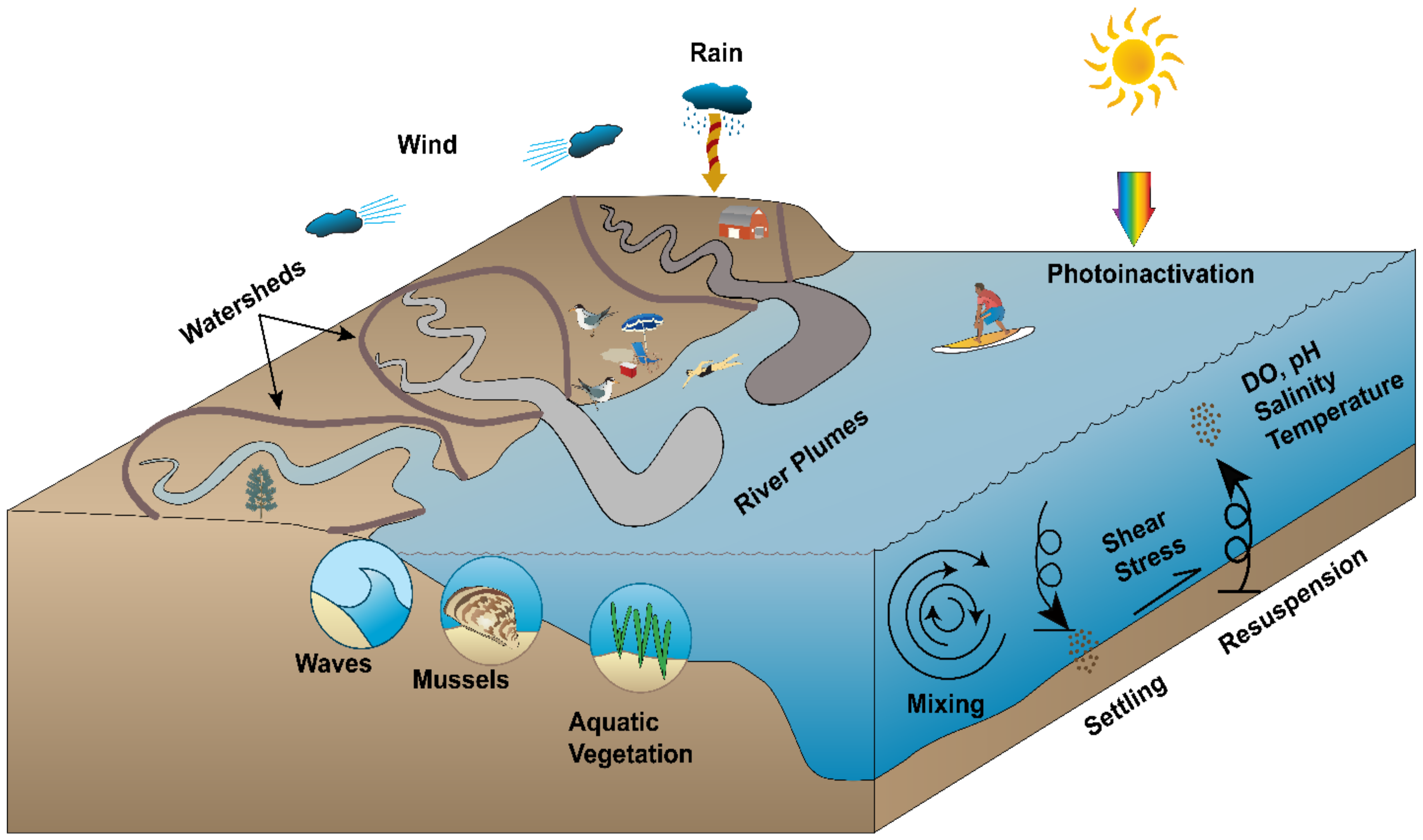
Table 1.
Base mortality terms used in contaminant fate and transport models.
| Aquatic Environment Type | Simulated Microorganism | Base Mortality Term | Reference |
|---|---|---|---|
| Freshwater/Marine | E. coli | Mancini [59] | |
| Freshwater Lake/River | Coliform | Auer and Niehaus [85] | |
| Freshwater Lake/River | Fecal Coliform | Canale et al. [86] | |
| Freshwater Lake | E. coli, enterococci, Fecal Coliform | Jin et al. [74] | |
| Freshwater Lake/River | E. coli | Jamieson [87] | |
| Brackish Lake | Fecal Coliform | McCorquodale et al. [81] | |
| Estuary/Coastal | Total Coliform | Kashefipour et al. [44] | |
| Estuary/Coastal | Fecal Coliform | Kashefipour et al. [44] | |
| Generic Coastal Model | Generic Bacteria, Viruses, Protozoa | Hipsey et al. [21] | |
| Freshwater Stream | E. coli | Rehmann and Soupir [78] | |
| Freshwater Lake | E. coli | Thupaki et al. [15] | |
| Estuary/Coastal | E. coli | Servais et al. [82,83]; De Brauwere et al. [84] | |
| Estuary/Coastal | E. coli | Bedri et al. [88] | |
| Estuary/Coastal | Fecal Coliform | Liu et al. [76] | |
| Freshwater Lake | E. coli | Thupaki et al. [35] | |
| Estuary/Coastal | Vibrio spp. | Froelich et al. [89] | |
| River/Estuary | Fecal Coliform | Boye et al. [90] | |
| Freshwater Lake | E. coli | Liu et al. [80] | |
| Freshwater Stream | Fecal Coliform | Reder et al. [91] | |
| Estuary/Coastal | Fecal Coliform | Gao et al. [45] | |
| Estuary/Coastal | Fecal Coliform | Liu et al. [77] | |
| Freshwater Lake | E. coli | Safaie et al. [16] | |
| Freshwater Lake | Fecal Coliform | Bravo et al. [20] | |
| Estuary/Coastal | E. coli | Garcia-Alba et al. [18] | |
| Freshwater Stream | E. coli | Mohammed et al. [51] |
Table 2.
Solar inactivation terms used in contaminant fate and transport models.
| Aquatic Environment Type | Simulated Microorganism | Solar Inactivation Term | Reference |
|---|---|---|---|
| Freshwater/ Marine | E. coli | Mancini [59] | |
| Freshwater Lake/River | Coliform | Auer and Niehaus [85] | |
| Freshwater Lake/River | Fecal Coliform | Canale et al. [86] | |
| Freshwater Lake | E. coli, enterococci, Fecal Coliform | Jin et al. [74] | |
| Brackish Lake | Fecal Coliform | McCorquodale et al. [81] | |
| Estuary/ Coastal | E. coli | Sanders et al. [73] | |
| Freshwater Lake | E. coli | Liu et al. [13] | |
| Estuary/ Coastal | Total Coliform, Fecal Coliform | Kashefipour et al. [44] | |
| Generic Coastal Model | Generic Bacteria, Viruses, Protozoa | Hipsey et al. [21] | |
| Freshwater Stream | E. coli | Rehmann and Soupir [78] | |
| Freshwater Stream | E. coli, enterococci | Cho et al. [97] | |
| Freshwater Lake | E. coli | Thupaki et al. [15] | |
| Freshwater Lake | E. coli | Thupaki et al. [35] | |
| Marine Coastal | Enterococci | Feng et al. [98] | |
| River/Estuary | Fecal Coliform | Boye et al. [90] | |
| Freshwater Lake | E. coli | Liu et al. [80] | |
| Freshwater Stream | Fecal Coliform | Reder et al. [91] | |
| Estuary/ Coastal | Fecal Coliform | Gao et al. [45] | |
| Marine Coastal | Enterococci | Feng et al. [99] | |
| Freshwater Lake | E. coli | Nekouee et al. [47,96] | |
| Freshwater Lake | E. coli | Safaie et al. [16] | |
| Freshwater Lake | Fecal Coliform | Bravo et al. [20] | |
| Estuary/ Coastal | E. coli | Garcia-Alba et al. [18] |
Table 3.
Sedimentation loss terms used in contaminant fate and transport models.
| Aquatic Environment Type | Simulated Microorganism | Sedimentation Loss Term | Reference |
|---|---|---|---|
| Freshwater Lake/River | Coliform | Auer and Niehaus [85] | |
| Freshwater Lake/River | Fecal Coliform | Canale et al. [86] | |
| Freshwater Lake | E. coli, enterococci, Fecal Coliform | Jin et al. [74] | |
| Brackish Lake | Fecal Coliform | McCorquodale et al. [81] | |
| Freshwater Lake | E. coli | Liu et al. [13] | |
| Generic Coastal Model | Generic Bacteria, Viruses, Protozoa | Hipsey et al. [21] | |
| Freshwater Stream | E. coli | Rehmann and Soupir [78] | |
| Freshwater Stream | E. coli, enterococci | Cho et al. [97] | |
| Freshwater Lake | E. coli | Thupaki et al. [15] | |
| Estuary/Coastal | E. coli | De Brauwere et al. [84] | |
| Estuary/Coastal | Fecal Coliform | Liu et al. [76] | |
| Freshwater Lake | E. coli | Thupaki et al. [35] | |
| Freshwater Lake | E. coli | Liu et al. [80] | |
| Freshwater Stream | Fecal Coliform | Reder et al. [91] | |
| Estuary/Coastal | Fecal Coliform | Liu et al. [80] | |
| Freshwater Lake | E. coli | Safaie et al. [16] | |
| Freshwater Lake/River | E. coli | Liu [38] |
Table 4.
Skill statistics and validation data for published numerical models of microbial water quality and FIO fate and transport.
Table 4.
Skill statistics and validation data for published numerical models of microbial water quality and FIO fate and transport.
| Aquatic Environment Type | Simulated Microorganism | Validation Type/Statistic | Skill Statistic Value/Qualitative Observations | Reference |
|---|---|---|---|---|
| Freshwater/Marine | E. coli | Qualitative Evaluation | Good agreement with coliform mortality rates. | Mancini [59] |
| Freshwater Lake/River | Coliform | Qualitative Evaluation | Model was based on empirical relationships from lab/field data. | Auer and Niehaus [85] |
| Freshwater Lake/River | Fecal Coliform | Qualitative Evaluation | Model output is comparable and consistent with observed bacterial loads during wet and dry weather events. | Canale et al. [86] |
| Freshwater Lake | E. coli, enterococci, Fecal Coliforms | Qualitative Evaluation | Fairly good prediction of observed microbial concentrations, but a general underestimation by the model. | Jin et al. [74] |
| Freshwater Lake/River | E. coli | Qualitative Evaluation | Modeled results generally simulate observations well. Empirical data should be used to calibrate models for nutrient-rich streams. | Jamieson [87] |
| Brackish Lake | Fecal Coliforms | Qualitative Evaluation | Fecal coliform dilution-decay is well-represented in the model, but predictions are susceptible to high levels of uncertainty associated with observed values. | McCorquodale et al. [81] |
| Estuary/ Coastal | E. coli | R2 | 0.19–0.70 | Sanders et al. [73] |
| Freshwater Lake | E. coli | RMSE | 0.71–0.84 | Liu et al. [6] |
| Estuary/Coastal | Total Coliform | R2 | 0.715 | Kashefipour et al. [44] |
| Estuary/Coastal | Fecal Coliform | R2 | 0.686 | Kashefipour et al. [44] |
| Generic Coastal Model | Generic Bacteria, Viruses, Protozoa | Qualitative Evaluation | The generic model did not outperform other models significantly. | Hipsey et al. [21] |
| Freshwater Stream | E. coli | Qualitative Evaluation | Predictive capacity changes over time. Model underpredicts E. coli at shorter time scales but reproduces measurements at longer time scales after storms. | Rehmann and Soupir [78] |
| Freshwater Stream | E. coli, enterococci | NSE | −0.02–0.81 | Cho et al. [97] |
| Freshwater Lake | E. coli | RMSE | 0.41 | Thupaki et al. [15] |
| Estuary/Coastal | E. coli | Qualitative Evaluation | Reference model overpredicted median observations by 7 and 3% at Temse and Uitbergen locations, respectively, but the variability of modeled results is much higher (3% for Uitbergen, 50% for Temse) than the observed data. | De Brauwere et al. [84] |
| Estuary/Coastal | E. coli | Qualitative Evaluation | Model significantly underestimates E. coli in a bay. | Bedri et al. [88] |
| Estuary/Coastal | Fecal Coliform | R2 | 0.71–0.83 | Liu et al. [76] |
| Freshwater Lake | E. coli | RMSE | 0.52–1.36 | Thupaki et al. [35] |
| Estuary/Coastal | Vibrio spp. | RMSE | 0.80 | Froelich et al. [89] |
| Marine Coastal | Enterococci | Willmott Index of Agreement | 0.47–0.60 | Feng et al. [98] |
| Freshwater Lake | E. coli | NRMSE | 5–23 | Nekouee et al. [47,96] |
| River/Estuary | Fecal Coliform | MAE | 0.348 | Boye et al. [90] |
| Freshwater Lake | E. coli | RMSE | 2.24–3.00 | Liu et al. [80] |
| Freshwater Stream | Fecal Coliform | RMSE | 0.44–0.70 | Reder et al. [91] |
| Estuary/Coastal | Fecal Coliform | RMSE | 4.42–4.80 | Gao et al. [45] |
| Estuary/Coastal | Fecal Coliform | RMSE | 3.62–5.37 | Liu et al. [77] |
| Marine Coastal | Enterococci | RMSE MAE | 0.67–0.92 0.47–0.72 | Feng et al. [99] |
| Freshwater Lake | E. coli | R2 RMSE NSE | 0.60–0.72 0.52–0.60 0.13–0.30 | Safaie et al. [16] |
| Freshwater Lake/River | E. coli | RMSE/Qualitative Evaluation | Model was optimized for RMSE, given various Manning roughness coefficients. Optimized model used Manning roughness coefficient = 0.035. | Liu [38] |
| Freshwater Lake | Fecal Coliform | RMSE | 0.66 | Bravo et al. [20] |
| Estuary/Coastal | E. coli | R2 | 0.87 | Garcia-Alba et al. [18] |
| Freshwater Stream | E. coli | R2 | 0.26–0.31 | Mohammed et al. [51] |
© 2020 by the authors. Licensee MDPI, Basel, Switzerland. This article is an open access article distributed under the terms and conditions of the Creative Commons Attribution (CC BY) license (http://creativecommons.org/licenses/by/4.0/).
Share and Cite
MDPI and ACS Style
Weiskerger, C.J.; Phanikumar, M.S. Numerical Modeling of Microbial Fate and Transport in Natural Waters: Review and Implications for Normal and Extreme Storm Events. Water 2020, 12, 1876. https://doi.org/10.3390/w12071876
AMA Style
Weiskerger CJ, Phanikumar MS. Numerical Modeling of Microbial Fate and Transport in Natural Waters: Review and Implications for Normal and Extreme Storm Events. Water. 2020; 12(7):1876. https://doi.org/10.3390/w12071876
Chicago/Turabian StyleWeiskerger, Chelsea J., and Mantha S. Phanikumar. 2020. "Numerical Modeling of Microbial Fate and Transport in Natural Waters: Review and Implications for Normal and Extreme Storm Events" Water 12, no. 7: 1876. https://doi.org/10.3390/w12071876
Note that from the first issue of 2016, this journal uses article numbers instead of page numbers. See further details here.