Stochastic Open-Pit Mine Production Scheduling: A Case Study of an Iron Deposit


1
Department of Metallurgical and Mining Engineering, Universidad Católica del Norte, Antofagasta 1270709, Chile
2
Advanced Mining Technology Center, University of Chile, Santiago 8370448, Chile
3
Department of Mining Engineering, University of Chile, Santiago 8370448, Chile
4
Delphos Mine Planning Laboratory, Department of Mining Engineering, Universidad de Chile, Santiago 8370448, Chile
*
Author to whom correspondence should be addressed.
Minerals 2020, 10(7), 585; https://doi.org/10.3390/min10070585
Submission received: 4 May 2020
/
Revised: 23 June 2020
/
Accepted: 26 June 2020
/
Published: 29 June 2020
(This article belongs to the Special Issue Geological Modelling, Volume II)
Abstract
:Production planning decisions in the mining industry are affected by geological, geometallurgical, economic and operational information. However, the traditional approach to address this problem often relies on simplified models that ignore the variability and uncertainty of these parameters. In this paper, two main sources of uncertainty are combined to obtain multiple simulated block models in an iron ore deposit that include the rock type and seven quantitative variables (grades of Fe, SiO2, S, P and K, magnetic ratio and specific gravity). To assess the effect of integrating these two sources of uncertainty in mine planning decision, stochastic and deterministic production scheduling models are applied based on the simulated block models. The results show the capacity of the stochastic mine planning model to identify and minimize risks, obtaining valuable information in ore content or quality at early stages of the project, and improving decision-making with respect to the deterministic production scheduling. Numerically speaking, the stochastic mine planning model improves 6% expected cumulative discounted cash flow and generates 16% more iron ore than deterministic model.
1. Introduction
Mineral resources evaluation and long-term mine planning are two of the most important steps in a mining project. Considering an ore deposit that will be mined on the surface (open pit mine), the following steps are essential to decide which part of the deposit should be extracted and when:
- geological block modeling: data are obtained from the geological logging and analytical assays of drill hole samples taken at different locations and depths in the deposit, and are used to delineate lithological and mineralogical domains and to interpolate the grades of elements of interest (products, by-products and contaminants) and other attributes, such as the specific gravity and the metal recovery. This step usually combines expert geological knowledge with geostatistical methods. Then, the deposit is modeled as a three-dimensional array of rectangular cuboids or blocks, each of which is assigned a prediction of its grade(s) and other attributes (rock type, specific gravity, metal recovery, etc.) [1,2,3,4,5,6];
- economic model: based on the block model information, alternative destinations, such as mills, waste dumps or stockpiles, and economic parameters, such as metal prices, mining and processing costs, a specific economic value is assigned to each block, indicating the amount of money that one obtains or loses by extracting/processing this block;
- ultimate pit limit determination: this step consists of delimiting the sub-region of the deposit in which extraction will be carried out. Among many different possible configurations of blocks for extraction that respect the overall slope angle of pit walls, the configuration that maximizes the profit, termed the ultimate pit limit (UPL), is often chosen [7];
- production scheduling: this step consists of deciding which blocks should be extracted, and when, and how extracted blocks should be treated. For this purpose, the UPL is divided into smaller pits called nested pits. A sequence of pushbacks or phases is then defined by considering operational spaces. Finally, a long-term open-pit mine production scheduling (LOMPS) is defined, which considers a number of operational constraints in each phase and maximizes the cumulative discounted cash flow (DCF) of the project [7].
The steps described above are the traditional approach to generating a long-term open-pit mine production plan, which suffer from two drawbacks [8,9]. In particular, they only use a single block model of the deposit and, as a result, do not consider uncertainty in the geological properties such as the metal grades. In fact, this model is just a prediction of reality and always differs from it. As a consequence, variations of the block model (e.g., by updating from new sampling information) cause changes in mine planning results. In addition, time is not considered as an important variable in determining the position of nested pits. These two drawbacks, among others, partly explain why mining companies are often unable to meet their production goals and financial prediction.
Mine planning is affected by several sources of uncertainty, one of the most important being the so-called geological uncertainty that refers to the delineation of lithological or mineralogical domains and the prediction of grades and other geological or geometallurgical attributes.
This study addresses stochastic geological modeling and stochastic long-term production planning of an open-pit mine using a two-stage approach through a real case study of a multi-element iron ore deposit. In the first stage, two main sources of uncertainty (on rock types and quantitative variables) are integrated in order to generate multiple block models. In the second stage, the block models from the first stage are used to generate a stochastic long-term mine plan. Finally, a comparison with the deterministic case is provided in order to evaluate the effect of these two sources of uncertainty in mine planning. The results show the capability of the proposed method to manage risk and to generate a higher expected cumulative DCF.
2. Background
2.1. Modeling Geological Uncertainty
Geostatistical simulation is now widely used to address uncertainty in subsurface models [5,6,9,10]. Unlike spatial prediction techniques such as kriging, simulation allows generating different outcomes, called realizations, of the deposit, each of which is a possible scenario. By having many different scenarios, it is possible to determine the level of uncertainty in the true unknown values of the attributes of interest. To date, many simulation models and algorithms have been designed, some of which are used for simulating quantitative variables measured on continuous scales, such as the metal grades or recoveries, while others are applicable to categorical variables, such as rock types or mineral zones [11,12,13].
Some important aspects to consider in the geostatistical modeling are: (1) the incorporation of data from different sources, (2) geological domaining and contact analysis to determine whether or not a quantitative variable exhibits clear-cut discontinuities when crossing a geological boundary, and (3) the modeling of the spatial dependence relationships between quantitative variables, as well as between quantitative and categorical variables. In particular, in case of hard geological boundaries, one can adopt a hierarchical approach where categorical and quantitative variables are simulated successively, whereas in case of soft boundaries, all these variables can be jointly simulated [14,15,16,17].
2.2. Production Scheduling under Geological Uncertainty
There are different approaches in applying simulated block models to mine planning, showing that geological uncertainty has important effects on the UPL and LOMPS stages. Most modeling approaches for the LOMPS problem under uncertainty are based on stochastic programming. One of the first efforts has been introduced in the context of mine planning by [18]: their model directly maximizes expected cumulative DCF and manages risk by minimizing deviations from ore, metal and/or mine production targets by penalizing the scenario-wise deviations (e.g., tonnage surplus or shortage) in the objective function. Some extensions and applications are documented in [19,20,21,22,23,24]. The reader is referred to [25] for a review of models and algorithms for long-term open-pit mine production planning, with and without considering parameter uncertainty.
Since the resulting optimization problems are large (usually involving millions of blocks and tens of periods), there are several approaches to solve them. These include from models supported on a well-defined mathematical framework, like multistage stochastic programming by [26], or based on risk control by using a chance-constrained programming model [27], to heuristics, where specific techniques are adapted (often, in a sequential manner) to find an optimal solution, or at least, a good feasible solution. Some approaches are based on genetic algorithms [28], simulated annealing [29], Tabu search [30], or variable neighborhood descent [31]. Heuristics based on time reduction have also been applied, like sliding time window heuristics [32,33] and linear programming relaxation based techniques [34,35]. Finally, block aggregation techniques have been proposed [36,37,38].
A common drawback of models that consider uncertainty in the ore content is that they only focus on grade uncertainty, without considering the other geological or geometallurgical attributes or interest for economic evaluation, mine planning and design, such as rock type domains, mineral zones, specific gravity or metal recovery [8,9]. It is important to quantify spatial uncertainty not only in metal grades, but also in volumes, tonnage and recoveries, which are used as input to mine planning [39]. One effort in this direction is the work in [40], which applies a two-step approach to quantify volumetric and multi-element grade uncertainty, generating 15 simulated scenarios as an input to mine planning. Unfortunately, the authors only present the stochastic production schedule and not a comparison with a deterministic case (without uncertainty).
3. Methodology
The following study is aimed at a preliminary economic assessment of an iron ore deposit and at assessing the impact of several sources of geological uncertainty on the discounted revenues along the life of the mine. First, one hundred outcomes (realizations) of the block model that represent the deposit (with information of rock types and quantitative variables) are generated, in order to quantify the uncertainty in the mineral resources. Then, a stochastic programming model is used to compute a single robust schedule by considering the set of outcomes under a multi-objective optimization approach to maximize the expected cumulative DCF and to quantify the risk of non-compliance of production targets. Finally, the stochastic approach is compared to a deterministic case. As the study focuses on a preliminary economic assessment of the project’s mineral resources, capital expenditure is not considered hereunder, reason for which the cumulative DCF is used as the economic indicator instead of the net present value (NPV) or the payback return period (PRP). Note, however, that the investment cost source is not subject to uncertainty and equally affects the mine plans obtained with both the stochastic and the deterministic approaches; therefore, it does not alter the comparison of these approaches.
In detail, the following steps are proposed to integrate geological uncertainty into stochastic mine planning:
- the layout of the geological domains (rock types) are simulated in the area of study, via the plurigaussian approach [12]. In this manner, it is possible to account for the uncertainty in the modeling of geological domains (rock type in this case);
- the quantitative variables of interest are jointly simulated within each simulated geological domain (obtained from the previous step) separately. Here, a multigaussian model together with a turning bands simulation algorithm [41] are used. By having multiple realizations, the uncertainty in the quantitative variables conditioned to the rock type model can be accounted for;
- a mixed stochastic integer programming (SIP) model is used to assess the impact of geological uncertainty. The model uses mine blocks along the planning horizon with the aim of maximizing the expected cumulative DCF and minimizing the total cost of uncertainty associated with deviations from production objectives (both in quantity and quality). The model is subject to several constraints such as precedence slope angles for safe pit walls, maximum and minimum operational resource consumption (mining and processing) associated with the quantity of materials, and maximum and minimum blending requirements, associated with the quality of the processed material;
- the approach for directly solving the SIP formulation is highly impractical at a large scale. To reduce the number of integer variables required by the SIP model, we use a temporal decomposition strategy to divide the original problem into sub-problems associated with fewer periods, together with a block pre-selection procedure based on a linear programming relaxation solution [42], but applied to a stochastic case.
A deterministic scheduling model (DIP, for deterministic integer programming) is applied on the model resulting from the averaging of all the simulated outcomes, in order to evaluate the ability of the SIP model to control the risk of non-compliance with production targets, as well as for comparison purposes.
4. Case Study
The proposed methodology was applied on a real case study (iron ore deposit). The uncertainty in the rock type and quantitative variables were modeled first using plurigaussian and multigaussian simulation, then, a stochastic open-pit production-scheduling model was applied for mine planning.
4.1. Presentation
In order to preserve data confidentiality, the location and the name of deposit are not disclosed, and each quantitative variable was multiplied by a constant prior to statistical analyses and geostatistical modeling. The area features volcanic rocks of calc-alkaline to alkaline composition, such as diorite-andesites, quartz monzonites-granodiorites, trachyandesites and rhyolites. The mineralization is related to surface and silicified igneous events that can be classified as late magmatic to early hydrothermal processes responsible for fluid phases rich in iron and associated with contact mineralization. The primary ore consists mainly of magnetite, pyrite, chalcopyrite and small amounts of bornite and hematite, while the gangue is composed of calcite, gypsum, plagioclase, potassium feldspar, quartz and contact minerals like clindenophoxenes of hedenbergitic, actinolite, epidote, garnet and apatite. The present alterations are argilization, epidotization, chloritization, silicification, and oxidation, the latter associated with mineral zones.
The geological modeling considers three lithological domains:
- host rock, composed mostly of intrusive or hypabyssal rocks such as andesites, diorites and trachytes. These lithologies are porphyritic in texture and are affected by hydrothermal alteration, including argilization, epidotization and chloritization. The iron grades are low, generally less than 14.5%;
- skarn, formed by contact metamorphism at high temperatures and ductile rheological environments. This lithology contains epidote, chlorite, pyroxenes and clay minerals, as well as contact mineralization (magnetite) associated with faults and irregular fracturing, with an iron grade that reaches 25%;
- mineralized breccias, resulting from the cooling and fracturing of the skarn in a posterior event with lower temperature and a fragile rheological environment. The main iron ore mineral observed is magnetite, while the main gangue minerals are gypsum, chalcedony, mica and quartz.
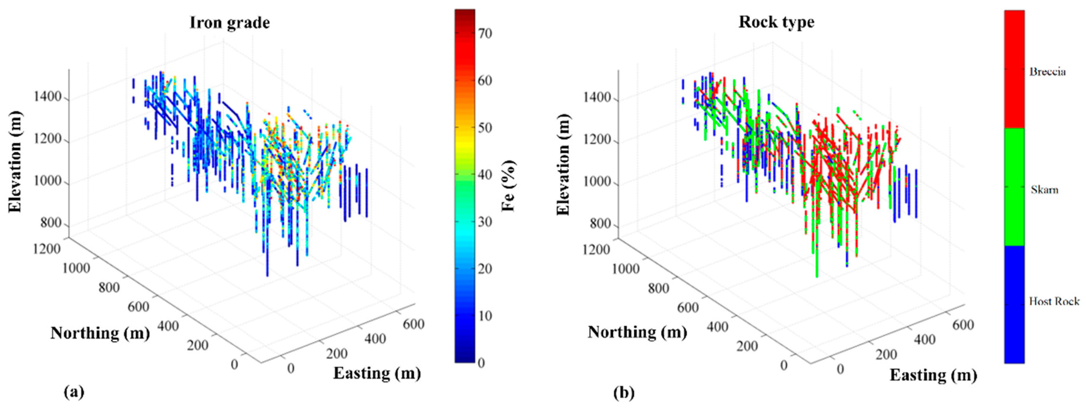
The available data consists of 5614 samples (gathered from 262 exploration diamond drill holes), composited at a length of 3 m, with information on the total grades of five elements (Fe, SiO2, S, P, K) and the magnetic ratio (MR) that quantifies the recovery of iron ore processing. The drill holes are mainly vertical and unevenly spaced (Figure 1).
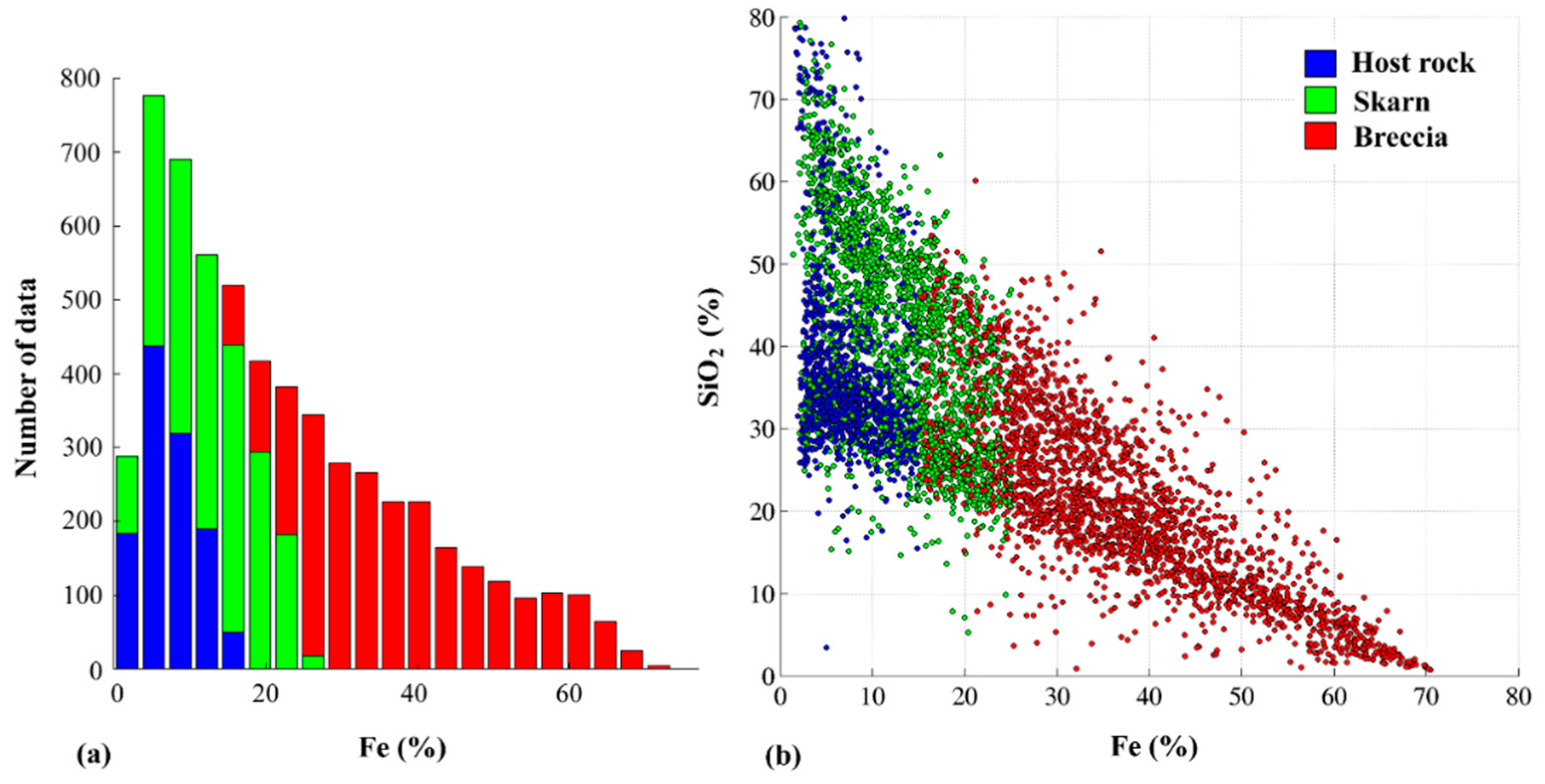
The distribution and main statistical parameters of the variables in the entire deposit and in each rock type are presented in Table 1 and Figure 2a. The distribution of iron grade (the main product of interest) turns out to be controlled by the three rock type groups that are present in the region under study, because the host rock is low in grade while the breccia is high-grade, and also because the dependence relationships between grades are differentiated (Figure 2b). The control of the rock type on the distribution of grades suggests that the uncertainty in the rock type layout can have a strong impact on the uncertainty in the iron grade and the other quantitative variables. This condition implies that the uncertainty in the rock type model cannot be omitted when modeling the quantitative variables.
4.2. Rock Type Modeling
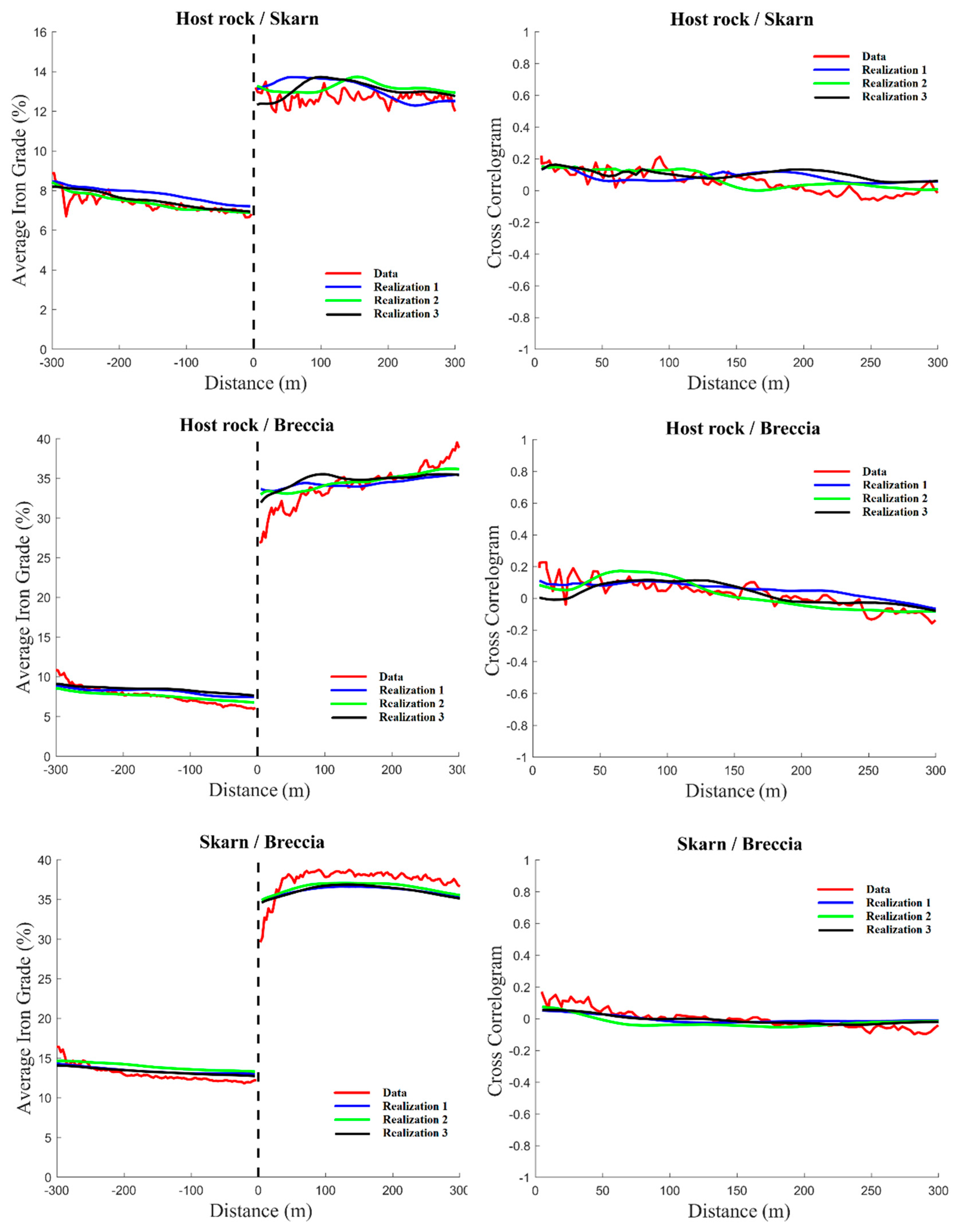
A contact analysis was performed to determine the most appropriate approach to combine rock type uncertainty with grade uncertainty. This analysis (Figure 3) shows the presence of hard boundaries (clear-cut discontinuities in the grade variations) between rock types. Therefore, it was decided to use a hierarchical approach in which the rock type domains are simulated first, with quantitative variables being subsequently simulated within each domain [14,15].
In the first step, the layout of the rock types in the region under study was simulated based on a plurigaussian model. Specifically, the truncation of a first synthetic Gaussian random field defines the space occupied by the host rock. The remaining space is split into skarn and breccia according to the truncation of a second, independent, Gaussian random field. Such a truncation rule is consistent with geological knowledge according to which breccia has formed by the fracturing and brecciation of the skarn. The truncation thresholds and the spatial structure of the Gaussian random fields are defined on the basis of the mean values and variograms of the rock type indicators, respectively [12].
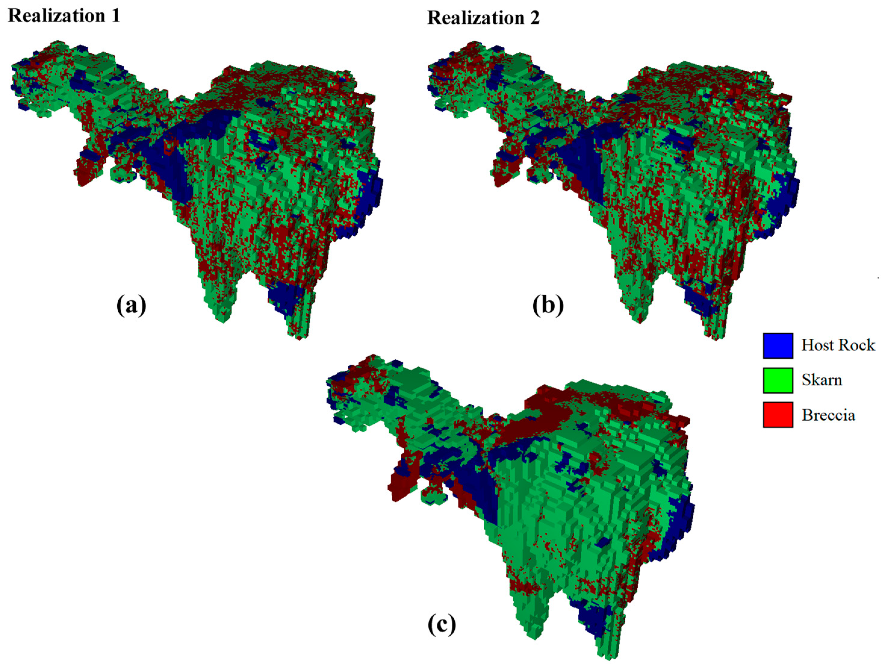
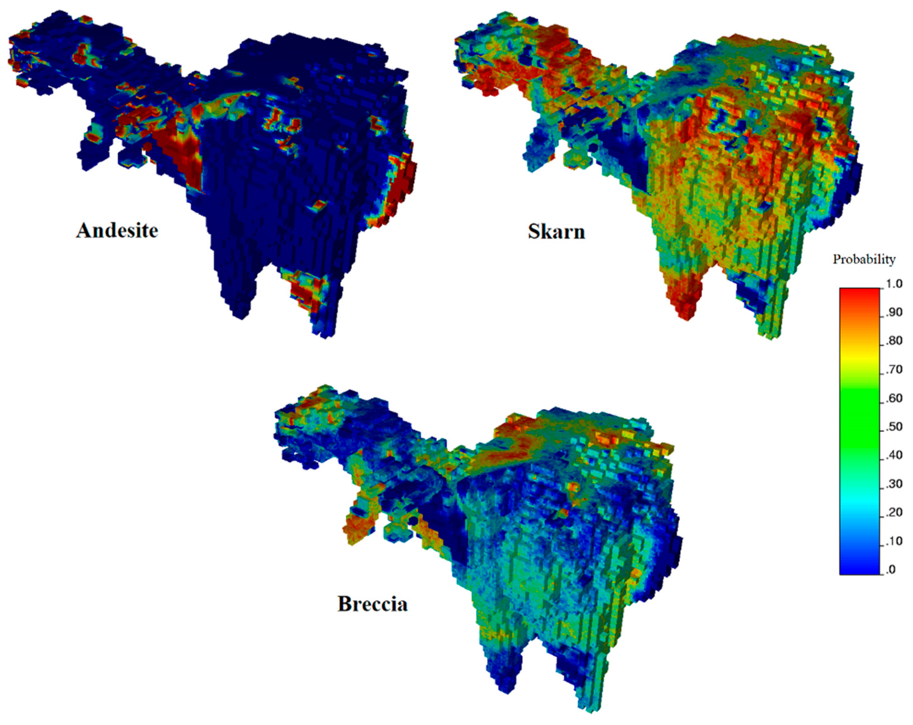
Details of the simulation algorithm can be found in the literature [12]. One hundred realizations of the rock type layout were generated on a grid with mesh 3.33 m × 3.33 m × 3.33 m and conditioned to the sampling data. Two realizations are shown in Figure 4a,b, while Figure 4c displays the most probable rock type for each grid node, determined on the basis of all the realizations. The latter appears smoother than the former, insofar as each individual realization is designed to reproduce the spatial variability of the rock type domains, not to predict them accurately. The uncertainty in the rock type occurrence can be assessed through probability maps, by calculating, at each grid node, the frequency of each rock type over the 100 realizations (Figure 5).
4.3. Modeling of Quantitative Variables
In each rock type, the quantitative variables (Fe, SiO2, S, P, K, MR) were normal-score transformed. The experimental direct and cross-variograms of the normal scores data were then calculated. The fitting of theoretical variogram models was realized as per the following strategy:
- for the host rock, a linear coregionalization model was fitted for all the quantitative variables of interest using a semi-automated least-square algorithm [43];
- for the skarn domain, a linear coregionalization model was fitted for Fe, SiO2, K and MR, and other two models were fitted for S and P, insofar as none of these variables present significant correlations with the remaining ones in this domain;
- for the mineralized breccia, a linear coregionalization model was fitted for all the variables of interest except S, which was modeled separately.
One hundred realizations (each one associated with a different rock type realization) were generated using a turning bands algorithm [41] on the same grid with mesh 3.33 m × 3.33 m × 3.33 m. The rock types were treated separately and the realizations in each rock type were conditioned to the data that belong to that rock type, in agreement with the contact analysis that shows the presence of hard geological boundaries. The variations of mean grade as a function of the distance to the geological boundaries, as well as the cross-correlation of grades across the rock types, are well reproduced (Figure 3). A cross-validation was also performed in order to check the global and conditional unbiasedness of the simulation.
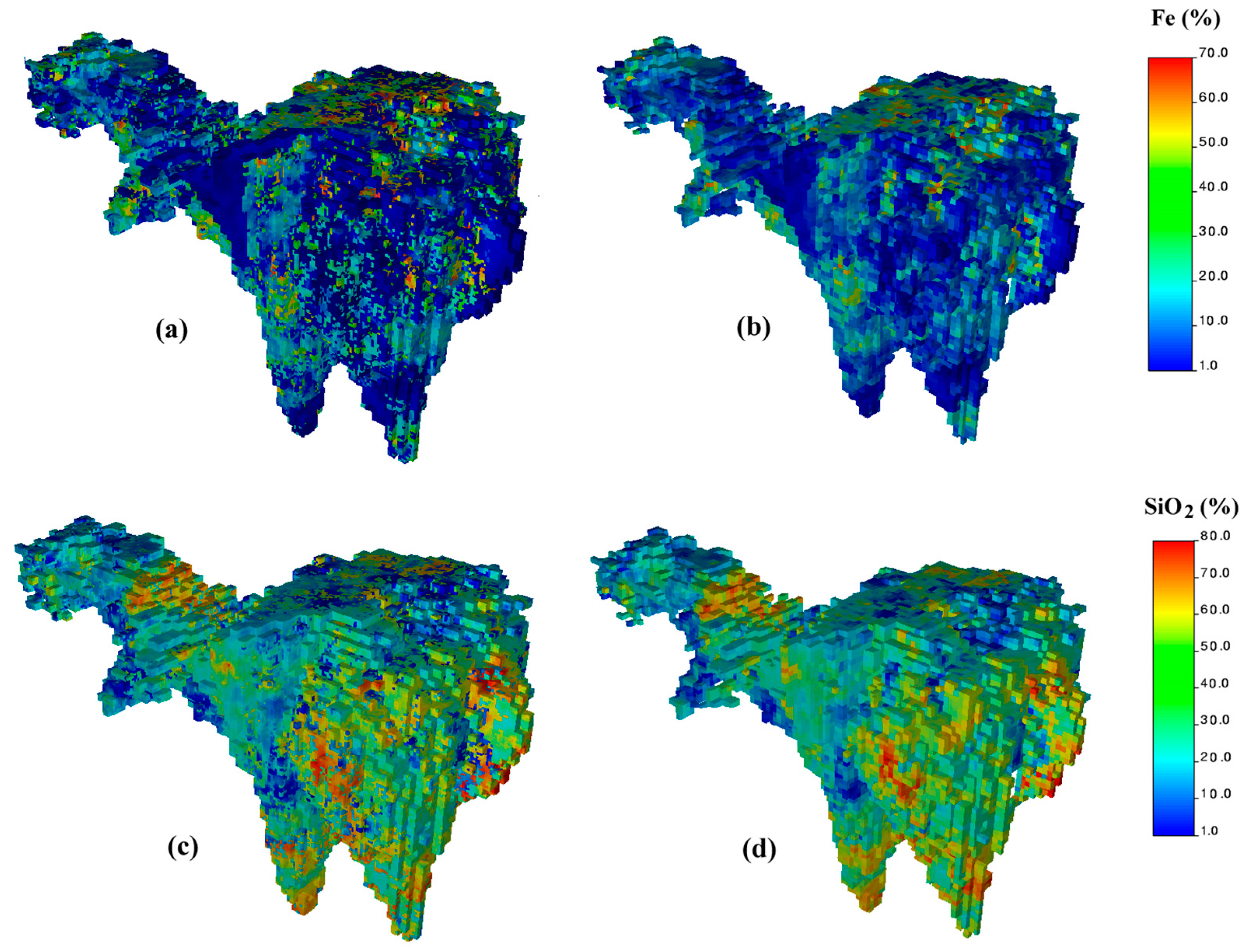
At this stage, the simulated grades have the same support as the composite sample data, i.e., a quasi-point support, and reproduce their distributions (histograms) and direct and cross-variograms (Figure 6a,c). The simulated grades were subsequently upscaled to the support of the selective mining unit (a block of size 10 m × 10 m × 10 m) by accounting for the specific gravity (SG), i.e., each block grade was calculated as a weighted average of the 27 point-support grades contained in the block, with a weight given by the specific gravity at the same grid node. The number of measurements of the specific gravity was too small to make a direct geostatistical modeling and simulation of this variable, but enough to identify its strong dependence relationship with the total iron grade and to fit a linear regression between both variables, assumed to be an accurate representation of reality:
SG = 2.112 + 0.0313 Fe
The magnetic ratio was not block-averaged directly. Instead, the recoverable iron grade was calculated at each node of the fine grid, as the product of the total iron grade with the magnetic ratio, then it was block-averaged by accounting for specific gravity. The block-support magnetic ratio was ultimately defined as the ratio between the block-support (upscaled) recoverable and total iron grades.
The proposed upscaling approach, based on a block discretization as suggested in [5,44,45], is preferred over the direct block-support simulation of the quantitative variables [46,47,48] because the latter assumes a single rock type per block and requires a change-of-support model (e.g., affine correction, discrete Gaussian model, or block-averaged covariance functions) that is suitable only for additive variables. Here, each block is discretized into 27 grid nodes that do not necessarily have the same rock type, thus allowing a mixed block composition, and the upscaling of grades is not additive since each grid node is weighted by the specific gravity when block averaging. The block-support realizations so obtained reproduce the joint distribution and the spatial correlation structure of the quantitative variables at this support; in particular, owing to the well-known support effect [3,5,6,13], they are smoother than the point-support realizations (Figure 6b,d).
4.4. Ultimate Pit Limit
In order to reduce the size of the block model, an ultimate pit limit was computed by considering the entire set of realizations. The economic block values were not only based on the profitable element (Fe), but also on the magnetic ratio and on the effects of undesirable elements, with the purpose of optimizing blending and penalizing profit when grades of different elements are higher or lower than the targets. This approach is especially useful in multi-element deposits such as those of iron ore (Appendix A).
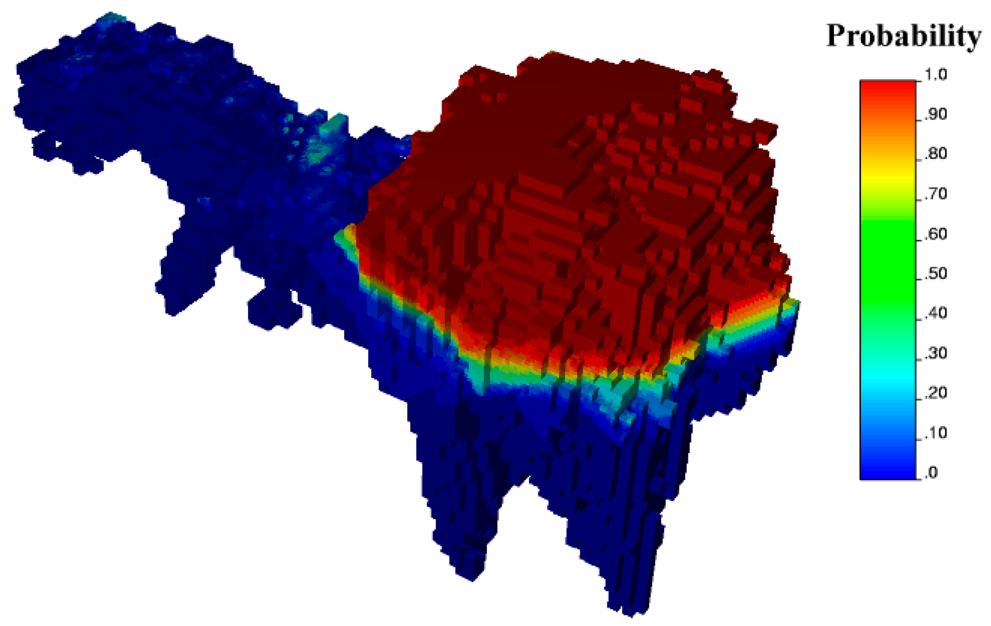
An ultimate pit limit was found for each realization. From the set of realizations, each block was assigned a probability to belong to the ultimate pit (Figure 7) and a 95% probability threshold was chosen to delineate the ultimate pit to be used for production scheduling. Given that the deposit has low to medium iron grade and contains several high-graded contaminants, this pit is restricted to a small portion located in the southern sector of the deposit. On average over the 100 realizations, it contains about 405 Mton of total material, divided into 108 Mton of ore and 297 Mton of waste (Table 2). The most probable rock domain composition in the pit limits is: 2% host rock, 27% skarn and 71% breccia, as expected because breccia has the highest iron grade and magnetic ratio.
4.5. Production Scheduling
We used a stochastic mixed-integer programming (SIP) model as presented in Appendix B to generate a production schedule. A hypothetical production-planning horizon of 12 periods was considered to schedule 405 Mton of expected total material for extraction and 108 Mton of expected ore for processing, as detailed in Table 2. To control this schedule, a mining capacity of 36 Mton/year and a processing capacity of 9.5 Mton/year were imposed. Quality was controlled per period: limits for iron blending grade were between 30.0% and 62.0%, while only upper boundaries were applied for impurities: SiO2 < 15%, S < 0.2%, P < 0.6%, K < 1.2%. The reason for this decision is that no penalties or bonuses were applied for low impurity content in iron ore. Penalties for shortage and/or surplus deviations of production targets were computed according to Mai’s approach [38], which guarantees that the total costs of producing shortage and/or surplus deviations from production targets (iron ore production and grades of (un)desirable elements) are higher than the benefits gained. A discount rate of 10% was applied on revenues and costs.
The results of the stochastic schedule are presented below, with an evaluation of the capacity of the SIP model to control risks associated with geological uncertainty. The results are in terms of production objectives: total and ore tonnes, and blending grades of the different elements, on average, while considering risk profiles by means of error bars (5th and 95th percentiles, henceforth, P5 and P95 for simplicity) when the stochastic schedule is assessed using the set of simulated block models. We furthermore compared SIP to the deterministic scheduling model (DIP) (Appendix C) applied to the most probable rock domain and average grade model as the geological model inputs. To ensure a fair comparison of the SIP and DIP models, the same economic parameters for block valuation and technical parameters for slope precedence, operational resource consumption and grade blending were used.
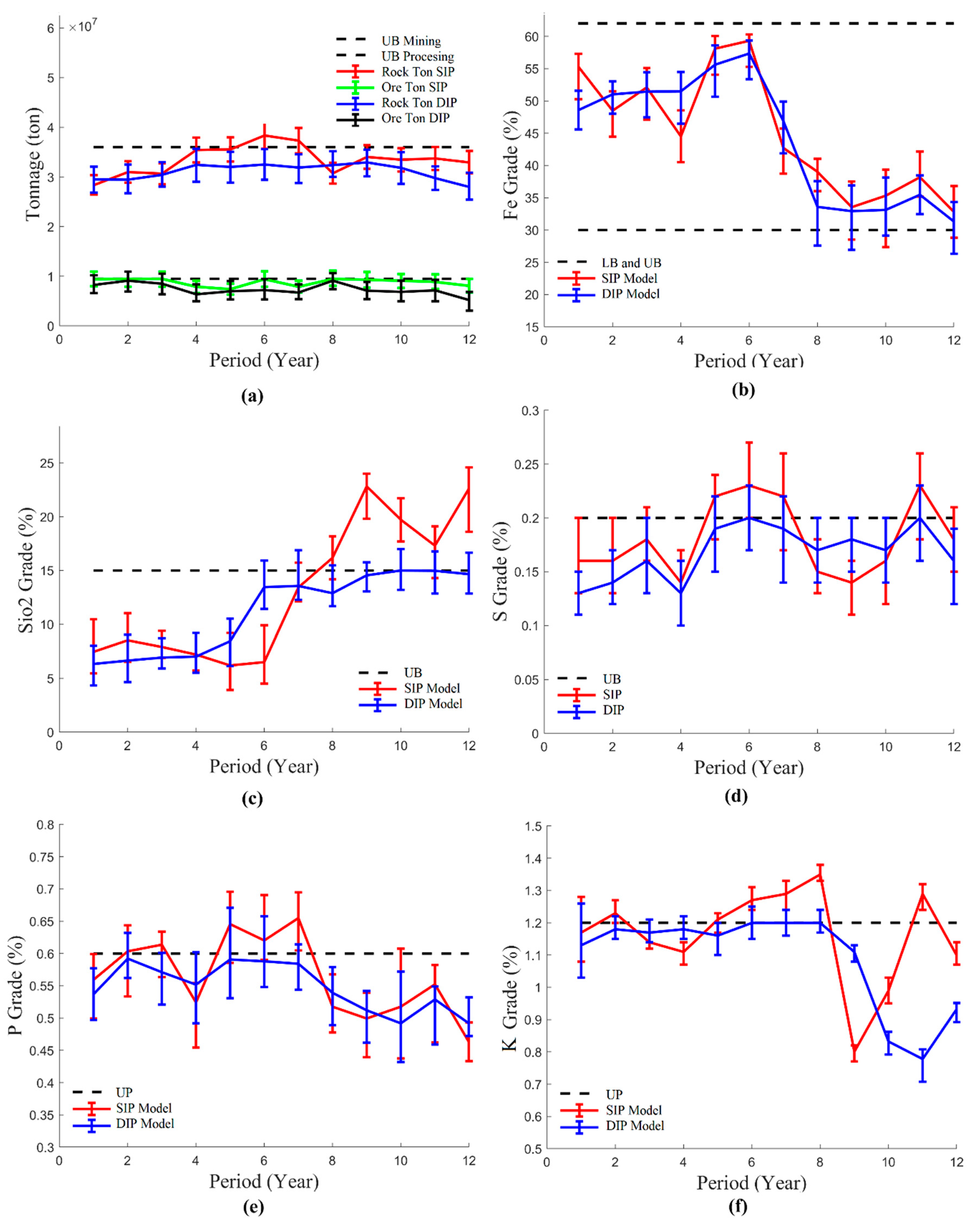
Figure 8 compares the production scheduling performance of the SIP and DIP models. Figure 8a shows ore production (green line) and total tonnes (red line) per year. No minimum boundary is imposed on resource consumption: the schedule that maximizes cumulative DCF always seeks to achieve the maximum processing capacity. However, in periods 6 and 7, the model exceeds the maximum mining capacity by 5% on average, to maximize iron ore production as much as possible, because the costs associated with that deviation are less than the perceived benefits of more iron ore production, and there is a possible deviation in total tonnage in periods 4 and 5. This uncertainty in total tonnage is due to variations in rock specific gravity in the rock domain simulations. In terms of ore production, the schedule shows that it is highly probable to meet the production target of 9.5 million tonnes. In the deterministic case, a lower productivity (on average) is obtained: 16% in ore tonnes (black line) and 7% in total rock (blue line), when compared with the stochastic schedule: This is because the DIP model must adhere to hard constraints (Equations (A17)–(A22) in Appendix C) and has to reach additional material that does not satisfy blending constraints.
Figure 8b shows the iron grade (SIP, red line) and its upper and lower limits (black lines) over the time periods. The first six periods present the higher grades, particularly periods 5 and 6. The required iron grade is met in most periods, with the exception of the end of the planning horizon in periods 9, 10 and 12, where there is a probability of 6% that the schedule does not meet the minimum quality requirements of the processed material. High grades in periods 5 and 6 explain why the SIP model tries to saturate the processing capacity as much as possible, even if it deviates from the upper mining boundary.
Regarding undesirable elements in iron ore, Figure 8c–f reports the expected behavior of silica (SiO2), sulfur (S), phosphorus (P) and potassium (K) and their risk profiles. Silica (Figure 8c), one of the most important impurities to be controlled, shows deviations from period 8 to 12, with a high probability of non-compliance of the silica production target. The predominant rock type in the ore reserve is breccia, where Fe and SiO2 correlate negatively. It follows that low (high) SiO2 grades are present in periods with high (low) Fe grades. Figure 8d shows sulfur content and the most likely deviations in periods 5, 6, 7 and 11. Similarly, Figure 8e reports phosphorus content in the iron ore, with slight deviations reported in periods 2 and 3, and the most likely deviations in periods 5 to 7 also being observed. Finally, Figure 8f presents potassium content per period, showing the most likely deviations in periods 1, 6, 7, 8 and 11. These deviations reduce the selling price of the iron ore because additional processes are required to reduce impurities.
In this sense, the SIP model allows for deviations, but controls the associated cost of accepting iron ores with high levels of impurities, always seeking the schedule that maximizes cumulative DCF, while minimizing the cost of deviating from production targets. In terms of ore control, the DIP model presents higher deviations in iron grade in the later periods, and anticipates surplus deviations in silica grade. Other contaminants show better performance, but at the cost of lower productivity, and therefore a lower expected cumulative DCF.
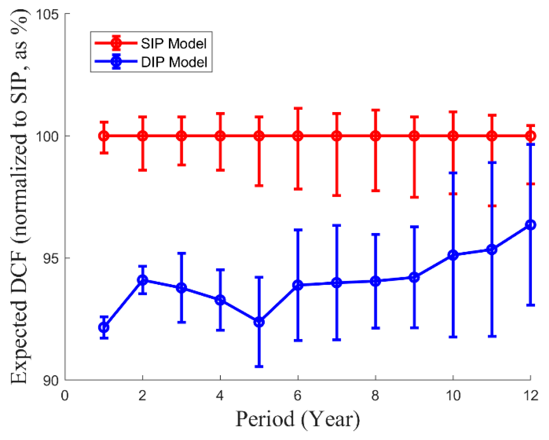
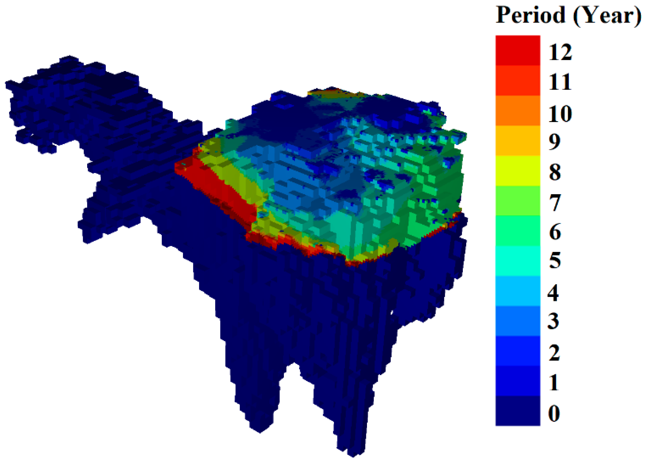
Figure 9 shows the expected cumulative DCF for the production schedule of the DIP model compared to that of the SIP model, which is used as a reference (100 as percentage), yielding a value 6% lower than what is expected using a 10% discount rate. Figure 10 shows the mining extraction sequence obtained from production schedule by the SIP model, with an isometric view. Finally, a summary of the pros and cons of each model (SIP and DIP) found during this study is presented in Table 3.
5. Conclusions and Perspectives
This work compared stochastic and deterministic mine planning under geological uncertainty using a real iron ore deposit as a case study. Detailed geological modeling included rock types and quantitative variables (multi-element grades of iron ore and impurities, as well as the magnetic ratio) as two sources of uncertainty in a two-step hierarchical approach. First, the uncertainty in the rock types in the studied area was modeled by applying plurigaussian simulation. Then, the values of five quantitative variables were simulated jointly in each rock type, yielding one hundred realizations each, which were averaged to a block size of 10 m × 10 m × 10 m, accounting for a non-constant specific gravity (a function of the iron grade).
The stochastic mine planning model allows for deviations, but controls the associated cost of accepting iron ore tonnes with higher impurity contents. As a result, this model obtained the schedule that simultaneously maximizes expected profits and minimizes the risk of losses due to deviations from production objectives. The results show that the stochastic approach has a high probability of meeting production targets in terms of ore production, improving ore output by 16% on average, and consequently, increasing profits by 6% on average, compared to the deterministic case. Regarding the grade profile, it is generally shown that the stochastic model manages well the grades in the first periods, which is consistent given that the discount rate affects the objective of maximizing profits. However, the element of interest and contaminant grades is highly variable, especially in the later periods, which should be taken into consideration in the project evaluation.
The scope of the case study was a preliminary economic assessment of the deposit and all the analyses were based on the geological properties of the ore (rock types, specific gravity, grades and magnetic ratio), metal price and operational expenditure (mining, processing and selling costs, which depend on the rock and metal tonnes, subject to geological uncertainty). The proposed stochastic programming approach can be further enriched in order to define the ore reserves requested for prefeasibility and feasibility studies, by classifying the mineral resources into measured, indicated and inferred—the latter not being part of the reserves—and considering other modifying factors to convert resources into reserves, such as water/energy availability, socio-political and environmental restrictions, government taxes, royalty, licenses fees and capital expenditure. At the (pre)feasibility stage where initial investment assumptions are required, the cumulative discounted cash flow can be substituted with other economic indicators such as the net present value and payback return period. Uncertainty can also be assigned to the modifying factors, in particular to the commodity prices, the foreign exchange rates and the operational costs, which vary in time. One of the most important challenges in this research line (mine planning under market uncertainty) is the availability of robust models that properly capture the behavior of prices and costs over time, beyond evaluating a few scenarios (pessimistic, average, optimistic), as usually done. Real options valuation is an interesting approach to be included in this future research line [49,50].
Author Contributions
M.M., E.J. and X.E.: methodological development, designing and conducting the experiments and writing the paper. N.M.: methodological development. All authors have read and agreed to the published version of the manuscript.
Funding
the authors are grateful to two reviewers for their positive comments and acknowledge funding from the National Agency for Research and Development of Chile through grants CONICYT/FONDECYT/POSTDOCTORADO/N° 3180655 (M.M.), CONICYT/FONDECYT/REGULAR/N° 1170101 (X.E.) and CONICYT/PIA AFB180004 (E.J., X.E. and N.M.).
Conflicts of Interest
The authors declare no conflict of interest.
Appendix A. Economic Block Valuation
Let be the block model and denote blocks in by and . The block model has attributes such as rock types, specific gravity, grades of different elements and magnetic ratio. Each attribute has a set of conditional realizations. There is a set of production targets that must be controlled, such as rock and ore tonnages, and grades of interesting metal and contaminants. The index of production targets are: : rock tonnage, : ore tonnage, : Fe grade, : MR, : SiO2, : S grade, : P grade, : K grade.
If a block is classified as ore in realization , the block value is determined as:
Otherwise,
where with , is the metal price, , and are selling, processing and mining costs, respectively (note that mining and processing costs depend on the rock domains).
Since there is uncertainty in the rock domains, and respectively represent rock and ore tonnages for each block and realization , accounting for the specific gravity (an affine function of the iron grade) of this block in this realization. In terms of uncertainty in grades, represents the concentration of element , for each block and realization . is a penalization when the iron ore has an iron grade () lower than a minimum requirement (), and is the penalization applied when grade of an undesirable element exceeds the maximum limit .
Appendix B. Stochastic Integer Programming (SIP) Model
Consider the following notation: A planning horizon for an open-pit mine production schedule and a discounted block value if a block in realization is extracted at period considering a discount rate as given by . For shortage and/or surplus deviations from the production target , represent the unit costs, respectively, for each realization and period .
In order to control the quantity of mining resource consumed, lower and/or upper boundaries are imposed: for extraction, and for processing. The quality of different elements are controlled by using lower and/or upper boundaries: .
There are two kinds of variables, the first is for extraction decisions, is a binary variable equal to 1 if block is extracted in period t or before, and equal to 0 otherwise. The second is an auxiliary variable that represents the exact notion of a block extracted at period , defined as , and for . Other continuous variables, , are used to control deviations in production targets, represented in tonnes (shortage and surplus, respectively) of production objective , when considering realization and period . represents the subset of blocks with a precedence arc of block to control the slope pit walls.
By using a stochastic direct block scheduling approach, the production schedule for a set of realizations in a planning horizon can be found by solving the following problem:
The objective function (A3) has two parts: to maximize the expected total discounted profit of scheduled blocks throughout horizon , and to minimize the expected discounted cost associated with deviations from production objectives. Constraints (A4) ensure the set of precedence blocks must be extracted before block b can be extracted. Constraints (A5) ensure that each block can be extracted no more than once. Soft constraints (A6)–(A9) control the quantity of extracted tonnage and processed tonnages, and soft constraints (A10)–(A11) control the quality of blending each element , that are satisfied per period and realization . Finally, constraints (A12)–(A13) set the nature of variables. If all blocks in the ultimate pit limit must be extracted, then is an additional constraint.
Appendix C. Deterministic Integer Programming (DIP) Model
The DIP model is as follows:
where is the expected discounted block value throughout the set of realizations, for block in period . and are obtained from the most probable rock domain for each block . Finally, is the grade of element in average models over the 100 realizations for each block .
References
- Royer, J.J.; Mejia, P.; Caumon, G.; Collon, P. 3D and 4D geomodelling applied to mineral resources exploration—An introduction. In 3D, 4D and Predictive Modelling of Major Mineral Belts in Europe; Weihed, P., Ed.; Springer: Cham, Switzerland, 2015; pp. 73–89. [Google Scholar]
- Wellmann, F.; Caumon, G. 3-D structural geological models: Concepts, methods, and uncertainties. Adv. Geophys. 2018, 59, 1–121. [Google Scholar]
- Journel, A.; Huijbregts, C. Mining Geostatistics; Academic Press: London, UK, 1978; 600p. [Google Scholar]
- Sinclair, A.J.; Blackwell, G.H. Applied Mineral Inventory Estimation; Cambridge University Press: Cambridge, UK, 2002; 381p. [Google Scholar]
- Rossi, M.E.; Deutsch, C.V. Mineral Resource Estimation; Springer: Dordrecht, The Netherlands, 2014; 332p. [Google Scholar]
- Seéguret, S.A.; Emery, X. Géostatistique de Gisements de Cuivre Chiliens: 35 Années de Recherche Appliqueée; Presses des Mines: Paris, France, 2019; 264p. [Google Scholar]
- Hustrulid, W.A.; Kuchta, M.; Martin, R.K. Open Pit Mine Planning and Design; CRC Press: Boca Raton, FL, USA, 2013; 1298p. [Google Scholar]
- Dowd, P.; Xu, C.; Coward, S. Strategic Mine Planning and Design: Some Challenges and Strategies for Addressing Them. Min. Technol. 2016, 125, 22–34. [Google Scholar] [CrossRef]
- Dimitrakopoulos, R. Advances in Applied Strategic Mine Planning; Springer: Berlin/Heidelberg, Germany, 2018; 800p. [Google Scholar]
- Srivastava, R.M. Geostatistics: A toolkit for data analysis, spatial prediction and risk management in the coal industry. Int. J. Coal. Geol. 2013, 112, 2–13. [Google Scholar] [CrossRef]
- Lantueéjoul, C. Geostatistical Simulation: Models and Algorithms; Springer: Fontainebleau, France, 2002; 256p. [Google Scholar]
- Armstrong, M.; Galli, A.; Beucher, H.; Loc’h, G.; Renard, D.; Doligez, B.; Eschard, R.; Geffroy, F. Plurigaussian Simulations in Geosciences; Springer: Berlin/Heidelberg, Germany, 2011. [Google Scholar]
- Chilès, J.P.; Delfiner, P. Geostatistics: Modeling Spatial Uncertainty, 2nd ed.; Wiley Blackwell: Toronto, ON, Canada, 2012; 699p. [Google Scholar]
- Jones, P.; Douglas, I.; Jewbali, A. Modeling combined geological and grade uncertainty: Application of multiple-point simulation at the Apensu gold deposit, Ghana. Math. Geosci. 2013, 45, 949–965. [Google Scholar] [CrossRef]
- Mery, N.; Emery, X.; Cáceres, A.; Ribeiro, D.; Cunha, E. Geostatistical modeling of the geological uncertainty in an iron ore deposit. Ore. Geol. Rev. 2017, 88, 336–351. [Google Scholar] [CrossRef]
- Maleki, M.; Emery, X. Joint simulation of stationary grade and non-stationary rock type for quantifying geological uncertainty in a copper deposit. Comput. Geosci. 2017, 109, 258–267. [Google Scholar] [CrossRef]
- Emery, X.; Maleki, M. Geostatistics in the presence of geological boundaries: Application to mineral resources modeling. Ore. Geol. Rev. 2019, 114, 103124. [Google Scholar] [CrossRef]
- Ramazan, S.; Dimitrakopoulos, R. Traditional and new MIP models for production scheduling with in-situ grade variability. Int. J. Surf. Min. Reclam Environ. 2004, 18, 85–98. [Google Scholar] [CrossRef]
- Albor Consuegra, F.R.; Dimitrakopoulos, R. Stochastic mine design optimisation based on simulated annealing: Pit limits, production schedules, multiple orebody scenarios and sensitivity analysis. Min. Technol. 2009, 118, 79–90. [Google Scholar] [CrossRef]
- Ramazan, S.; Dimitrakopoulos, R. Production scheduling with uncertain supply: A new solution to the open pit mining problem. Optim. Eng. 2013, 14, 361–380. [Google Scholar] [CrossRef]
- Leite, A.; Dimitrakopoulos, R. Stochastic optimization of mine production scheduling with uncertain ore/metal/waste supply. Int. J. Min. Sci. Technol. 2014, 24, 755–762. [Google Scholar] [CrossRef]
- Goodfellow, R.C.; Dimitrakopoulos, R. Global optimization of open pit mining complexes with uncertainty. Appl. Soft. Comput. J. 2016, 40, 292–304. [Google Scholar] [CrossRef]
- Morales, N.; Seguel, S.; Cáceres, A.; Jélvez, E.; Alarcón, M. Incorporation of geometallurgical attributes and geological uncertainty into long-term open-pit mine planning. Minerals. 2019, 9, 108. [Google Scholar] [CrossRef] [Green Version]
- Nelis, G.; Morales, N.; Widzyk-Capehart, E. Comparison of different approaches to strategic open-pit mine planning under geological uncertainty. In Proceedings of the 27th International Symposium on Mine Planning and Equipment Selection—MPES 2018; Widzyk-Capehard, E., Hekmat, A., Singhal, R., Eds.; Springer: Cham, Switzerland, 2019; pp. 95–105. [Google Scholar]
- Osanloo, M.; Gholamnejad, J.; Karimi, B. Long-term open pit mine production planning: A review of models and algorithms. Int. J. Min. Reclam Environ. 2008, 22, 3–35. [Google Scholar] [CrossRef]
- Boland, N.; Dumitrescu, I.; Froyland, G. A Multistage Stochastic Programming Approach to Open Pit Mine Production Scheduling with Uncertain Geology. Optimization Online. 2008. Available online: http://www.optimization-online.org/DB_HTML/2008/10/2123.html (accessed on 27 June 2020).
- Vielma, J.P.; Espinoza, D.; Moreno, E. Risk control in ultimate pits using conditional simulations. In Proceedings of the 34th International Symposium on the Application of Computers and Operations Research in the Mineral Industry, Vancouver, Canada, 6–9 October 2009; pp. 567–575. [Google Scholar]
- Denby, B.; Schofield, D. Open-pit design and scheduling by use of genetic algorithms. Trans. Inst. Min. Metall. Sect. A 1994, 103, A21–A26. [Google Scholar]
- Godoy, M.; Dimitrakopoulos, R. Managing risk and waste mining in long-term production scheduling of open-pit mines. SME Trans. 2004, 316, 43–50. [Google Scholar]
- Lamghari, A.; Dimitrakopoulos, R. A diversified Tabu search approach for the open-pit mine production scheduling problem with metal uncertainty. Eur. J. Oper. Res. 2012, 222, 642–652. [Google Scholar] [CrossRef] [Green Version]
- Lamghari, A.; Dimitrakopoulos, R.; Ferland, J.A. A variable neighbourhood descent algorithm for the open-pit mine production scheduling problem with metal uncertainty. J. Oper. Res. Soc. 2014, 65, 1305–1314. [Google Scholar] [CrossRef] [Green Version]
- Cullenbine, C.; Wood, R.K.; Newman, A. A sliding time window heuristic for open pit mine block sequencing. Optim. Lett. 2011, 5, 365–377. [Google Scholar] [CrossRef] [Green Version]
- Adrien Rimélé, M.; Dimitrakopoulos, R.; Gamache, M. A stochastic optimization method with in-pit waste and tailings disposal for open pit life-of-mine production planning. Resour. Policy 2018, 57, 112–121. [Google Scholar] [CrossRef]
- Bienstock, D.; Zuckerberg, M. Solving LP relaxations of large-scale precedence constrained problems. In Lecture Notes in Computer Science (Including Subseries Lecture Notes in Artificial Intelligence and Lecture Notes in Bioinformatics); Eisenbrand, F., Shepherd, F.B., Eds.; Springer: Berlin, Germany, 2010; pp. 1–14. [Google Scholar]
- Samavati, M.; Essam, D.; Nehring, M.; Sarker, R. A new methodology for the open-pit mine production scheduling problem. Omega 2018, 81, 169–182. [Google Scholar] [CrossRef]
- Ramazan, S. The new Fundamental Tree Algorithm for production scheduling of open pit mines. Eur. J. Oper. Res. 2006, 177, 1153–1166. [Google Scholar] [CrossRef]
- Tabesh, M.; Askari-Nasab, H. Two-stage clustering algorithm for block aggregation in open pit mines. Trans. Inst. Min. Metall Sect. A Min. Technol. 2011, 120, 158–169. [Google Scholar] [CrossRef]
- Mai, N.L.; Topal, E.; Erten, O.; Sommerville, B. A new risk-based optimisation method for the iron ore production scheduling using stochastic integer programming. Resour. Policy 2019, 62, 571–579. [Google Scholar] [CrossRef]
- Dunham, S.; Vann, J. Geometallurgy, geostatistics and project value—Does your block model tell you what you need to know? In Proceedings of the Project Evaluation Conference, Melbourne, Australia, 19–20 June 2007; pp. 189–196. [Google Scholar]
- Vallejo, M.N.; Dimitrakopoulos, R. Stochastic orebody modelling and stochastic long-term production scheduling at the KéMag iron ore deposit, Quebec, Canada. Int. J. Min. Reclam Environ. 2019, 33, 462–479. [Google Scholar] [CrossRef]
- Emery, X. A turning bands program for conditional co-simulation of cross-correlated Gaussian random fields. Comput. Geosci. 2008, 34, 1850–1862. [Google Scholar] [CrossRef]
- Jélvez, E.; Morales, N.; Nancel-Penard, P.; Cornillier, F. A new hybrid heuristic algorithm for the Precedence Constrained Production Scheduling Problem: A mining application. Omega 2019, 102046. [Google Scholar] [CrossRef]
- Emery, X. Iterative algorithms for fitting a linear model of coregionalization. Comput. Geosci. 2010, 36, 1150–1160. [Google Scholar] [CrossRef]
- Glacken, I.M. Change of support and use of economic parameters for block selection. In Geostatistics Wollongong’ 96; Baafi, E.Y., Schofield, N.A., Eds.; Kluwer Academic: Dordrecht, The Netherlands, 1997; pp. 811–821. [Google Scholar]
- Journel, A.G.; Kyriakidis, P.C. Evaluation of Mineral Reserves: A Simulation Approach; Oxford University Press: Oxford, UK, 2004; 216p. [Google Scholar]
- Emery, X. Change-of-support models and computer programs for direct block-support simulation. Comput. Geosci. 2009, 35, 2047–2056. [Google Scholar] [CrossRef]
- Emery, X.; Ortiz, J.M. Two approaches to direct block-support conditional co-simulation. Comput. Geosci. 2011, 37, 1015–1025. [Google Scholar] [CrossRef]
- Zaytsev, V.; Biver, P.; Wackernagel, H.; Allard, D. Change-of-support models on irregular grids for geostatistical simulation. Math. Geosci. 2016, 48, 353–369. [Google Scholar] [CrossRef]
- Dimitrakopoulos, R.G.; Sabour, S.A. Evaluating mine plans under uncertainty: Can the real options make a difference? Resour. Policy 2007, 32, 116–125. [Google Scholar] [CrossRef]
- Akbari, A.D.; Osanloo, M.; Shirazi, M.A. Determination of ultimate pit limits in open mines using real option approach. IUST Int. J. Eng. Sci. 2008, 19, 23–38. [Google Scholar]
Figure 1.
Isometric views of drill hole data, colored according to (a) total iron grade, (b) rock type.
Figure 1.
Isometric views of drill hole data, colored according to (a) total iron grade, (b) rock type.

Figure 2.
(a) Histogram of iron grade and (b) scatter plot of iron vs. silica grades. Colors represent rock types.
Figure 2.
(a) Histogram of iron grade and (b) scatter plot of iron vs. silica grades. Colors represent rock types.

Figure 3.
Contact analysis between rock types. Left: mean iron grade as a function of the signed distance to the rock type boundary; right: cross-correlation between iron grades measured in different rock types, as a function of the distance between sampling data. Red line: original data; blue, green and black lines: simulated iron grades.

Figure 4.
(a,b) Two plurigaussian realizations of rock types conditioned to drill hole data. (c) Most probable rock type, i.e., the most frequent rock type over the realizations. White areas correspond to grid nodes above the topographic surface or outside the sampled region.
Figure 4.
(a,b) Two plurigaussian realizations of rock types conditioned to drill hole data. (c) Most probable rock type, i.e., the most frequent rock type over the realizations. White areas correspond to grid nodes above the topographic surface or outside the sampled region.

Figure 5.
Probability maps of the different rock types, calculated on the basis of 100 plurigaussian realizations.
Figure 5.
Probability maps of the different rock types, calculated on the basis of 100 plurigaussian realizations.

Figure 6.
One realization of iron (top) and silica (bottom) grades at (a,c) a quasi-point support (before upscaling) and (b,d) a block support (after upscaling).
Figure 6.
One realization of iron (top) and silica (bottom) grades at (a,c) a quasi-point support (before upscaling) and (b,d) a block support (after upscaling).

Figure 7.
Ultimate pit limit probability.

Figure 8.
Production plan obtained from the stochastic integer-programming (SIP) and deterministic integer programming (DIP) models: (a) ore and rock tonnes, and grades of (b) iron, (c) silica, (d) sulfur, (e) phosphorus, and (f) potassium. The error bars represent the P5 and P95 values obtained on the set of simulated block models; the continuous lines represent the average (expected) values.

Figure 9.
Expected discounted cash flow (DCF) from the DIP model compared to that of the SIP model as a reference case (100%). The error bars represent the P5 and P95 values obtained on the set of simulated block models; the continuous lines represent the average (expected) values.
Figure 9.
Expected discounted cash flow (DCF) from the DIP model compared to that of the SIP model as a reference case (100%). The error bars represent the P5 and P95 values obtained on the set of simulated block models; the continuous lines represent the average (expected) values.

Figure 10.
Extraction sequence (isometric view) along the planning horizon.


Table 1.
Statistics of the quantitative variables, globally and per rock type.
| Variable | Statistics | Global | Host Rock | Skarn | Breccia |
|---|---|---|---|---|---|
| Count | 5614 | 1177 | 2022 | 2415 | |
| Fe | Minimum | 1.40 | 1.56 | 1.40 | 15.02 |
| Maximum | 70.45 | 14.98 | 24.99 | 70.45 | |
| Mean | 21.82 | 7.17 | 12.62 | 36.82 | |
| Variance | 257.52 | 11.99 | 35.40 | 162.89 | |
| Median | 17.45 | 6.72 | 12.63 | 34.49 | |
| Upper Quartile | 31.82 | 9.57 | 17.24 | 45.15 | |
| Lower Quartile | 8.56 | 4.13 | 7.72 | 26.97 | |
| SiO2 | Minimum | 0.7 | 3.46 | 5.29 | 0.7 |
| Maximum | 83.11 | 83.11 | 79.31 | 60.1 | |
| Mean | 32.23 | 38.0 | 41.55 | 21.62 | |
| Variance | 226.07 | 142.57 | 160.26 | 121.10 | |
| Median | 31.13 | 34.18 | 41.42 | 20.84 | |
| Upper Quartile | 41.56 | 40.59 | 50.86 | 29.05 | |
| Lower Quartile | 22.107 | 30.75 | 30.55 | 13.37 | |
| S | Minimum | 0.007 | 0.02 | 0.4 | 0.007 |
| Maximum | 5.53 | 3.68 | 5.53 | 3.63 | |
| Mean | 0.594 | 0.45 | 0.62 | 0.64 | |
| Variance | 0.50 | 0.32 | 0.50 | 0.58 | |
| Median | 0.12 | 0.08 | 0.11 | 0.13 | |
| Upper Quartile | 0.21 | 0.20 | 0.21 | 0.22 | |
| Lower Quartile | 0.049 | 0.023 | 0.039 | 0.08 | |
| P | Minimum | 0.0 | 0.0 | 0.0 | 0.0 |
| Maximum | 11.1 | 8.5 | 11.1 | 9.45 | |
| Mean | 0.29 | 0.24 | 0.27 | 0.33 | |
| Variance | 0.22 | 0.18 | 0.24 | 0.21 | |
| Median | 0.46 | 0.29 | 0.48 | 0.52 | |
| Upper Quartile | 0.78 | 0.59 | 0.79 | 0.84 | |
| Lower Quartile | 0.26 | 0.15 | 0.30 | 0.32 | |
| K | Minimum | 0.0 | 0.35 | 0.018 | 0.0 |
| Maximum | 7.78 | 7.27 | 7.78 | 5.7 | |
| Mean | 2.05 | 2.70 | 2.33 | 1.5 | |
| Variance | 1.280 | 1.14 | 1.26 | 0.79 | |
| Median | 1.92 | 2.55 | 2.12 | 1.42 | |
| Upper Quartile | 2.7 | 3.31 | 2.88 | 2.07 | |
| Lower Quartile | 1.27 | 1.96 | 1.52 | 0.85 | |
| MR | Minimum | 0.0 | 0.0 | 0.0 | 0.0 |
| Maximum | 0.98 | 0.40 | 0.69 | 0.98 | |
| Mean | 0.22 | 0.05 | 0.11 | 0.41 | |
| Variance | 0.048 | 0.002 | 0.009 | 0.044 | |
| Median | 0.144 | 0.04 | 0.094 | 0.38 | |
| Upper Quartile | 0.34 | 0.06 | 0.15 | 0.55 | |
| Lower Quartile | 0.04 | 0.02 | 0.03 | 0.25 |
Table 2.
Summary statistics (average, 5th and 95th percentiles over 100 realizations of grades, specific gravity and magnetic ratio) of the ultimate pit included in the 95% pit limit probability.
Table 2.
Summary statistics (average, 5th and 95th percentiles over 100 realizations of grades, specific gravity and magnetic ratio) of the ultimate pit included in the 95% pit limit probability.
| Statistics | Rock Ton (Mton) | Ore Ton (Mton) | Waste Ton (Mton) | Stripping Ratio |
|---|---|---|---|---|
| P5 | 401.85 | 105.23 | 295.62 | 2.71 |
| Average | 404.88 | 107.72 | 297.16 | 2.74 |
| P95 | 409.26 | 109.06 | 298.47 | 2.78 |
Table 3.
Advantages and drawbacks of the SIP and DIP approaches.
| Approach | Advantages | Drawbacks |
|---|---|---|
| Stochastic integer programming (SIP) model | Geological and geometallurgical uncertainties are explicitly taken into account in the model. The model maximizes the expected cumulative discounted cash flow and, simultaneously, minimizes the impact of losses due to deviations from production targets. The solution under this approach has a better risk control and a higher probability of meeting production targets | Real-world size problems are computationally demanding (we applied a hybrid heuristic algorithm [42], allowing to reduce the required computer resources and running times). The choice of unit costs of under- and over-production strongly impacts the objective function (we followed the approach presented in [38]). Other sources of uncertainty such as commodity prices and costs are not considered. We propose this point as a future work. |
| Deterministic integer programming (DIP) model | This model lacks the possibility to deal with uncertainties in geological and geometallurgical variables: all the parameters used in the model are considered known in advance. The geological information is modeled through a single, smoothed block model (kriging prediction, or average of simulated realizations). Real-world size problems are computationally demanding. |
© 2020 by the authors. Licensee MDPI, Basel, Switzerland. This article is an open access article distributed under the terms and conditions of the Creative Commons Attribution (CC BY) license (http://creativecommons.org/licenses/by/4.0/).
Share and Cite
MDPI and ACS Style
Maleki, M.; Jélvez, E.; Emery, X.; Morales, N. Stochastic Open-Pit Mine Production Scheduling: A Case Study of an Iron Deposit. Minerals 2020, 10, 585. https://doi.org/10.3390/min10070585
AMA Style
Maleki M, Jélvez E, Emery X, Morales N. Stochastic Open-Pit Mine Production Scheduling: A Case Study of an Iron Deposit. Minerals. 2020; 10(7):585. https://doi.org/10.3390/min10070585
Chicago/Turabian StyleMaleki, Mohammad, Enrique Jélvez, Xavier Emery, and Nelson Morales. 2020. "Stochastic Open-Pit Mine Production Scheduling: A Case Study of an Iron Deposit" Minerals 10, no. 7: 585. https://doi.org/10.3390/min10070585
Note that from the first issue of 2016, this journal uses article numbers instead of page numbers. See further details here.