Seasonal Estuarine Turbidity Maximum under Strong Tidal Dynamics: Three-Year Observations in the Changjiang River Estuary


1
College of Harbor, Coastal and Offshore Engineering, Hohai University, Nanjing 210098, China
2
Key Laboratory of Coastal Disaster and Defence, Ministry of Education, Hohai University, Nanjing 210098, China
3
Shanghai Hydraulic Engineering Group Co., Ltd., Shanghai 201600, China
*
Author to whom correspondence should be addressed.
Water 2020, 12(7), 1854; https://doi.org/10.3390/w12071854
Submission received: 19 May 2020
/
Revised: 5 June 2020
/
Accepted: 13 June 2020
/
Published: 28 June 2020
(This article belongs to the Special Issue Observation and Modeling of Coastal Morphodynamics)
Abstract
:The estuarine turbidity maximum (ETM) under strong tidal dynamics (during spring tides) was investigated along the Deepwater Navigation Channel (DNC) in the North Passage (NP) of the Changjiang River Estuary (CRE) in wet and dry seasons of 2016, 2017 and 2018. The observed water current, salinity, stratification and suspended sediment concentration (SSC) were illustrated and analyzed. Results show that the SSC was lower in wet seasons than dry seasons in 2016 and 2017 because of the weak influence of typhoons before observations in wet seasons. On the contrary, the SSC was higher in the wet season than the dry season in 2018 because of the strong influence of typhoons in the wet season. Our observations challenged the common perspective that SSC in the NP is higher in wet seasons than dry seasons, because the magnitudes of SSC were found to be easily influenced by strong winds before observations. The along-channel distribution of high SSC was determined by the location of salt wedge, and consequently, the ETM was further upstream in dry seasons than wet seasons. The observed SSC was more concentrated in lower water layers in wet seasons (“exponential” profile) than dry seasons (“linear” profile). This seasonal difference of vertical SSC was related to the flocculation setting velocity influenced by temperature rather than the weak stratification during spring tides. Moreover, on the basis of the net water/sediment transport and flux splitting, large river discharge and a low-SSC condition could reduce siltation in the middle DNC. The former vanished the convergence of water transport, and the latter reduced landward tidal pumping sediment transport. Sediment trapping and siltation in the dry seasons occurred in the seaward segment of the upper reach because of the decrease in the river discharge.
1. Introduction
The estuarine turbidity maximum (ETM) refers to the region where the suspended sediment concentration (SSC) is higher than adjacent regions upstream and downstream. The sediment dynamics in the ETM exhibit significant difference among estuaries, depending on local topography, fluvial and tidal forcing, and sediment composition [1]. The formation mechanisms of the ETM, as reported by previous studies, can be attributed to estuarine circulation and residual current [2,3], tidal asymmetry [4,5], resuspension [4,6], stratification [7,8], flocculation [9,10] and sediment phase lag [11,12].
The Changjiang River Estuary (CRE), being the estuary of the largest river in China, is a mesotidal and partially mixed estuary with remarkable river discharges and strong tidal dynamics. The ETM in a partially mixed estuary is commonly related to sediment trapping [1,7,13]. In the North Passage (NP) of the CRE, where the Deepwater Navigation Channel (DNC) is located, sediment trapping is observed as the convergence of the near-bottom residual sediment [14,15,16]. In the upper reach of the NP, the seaward advective sediment transport dominates [15], while in the middle or lower reaches of the NP, the landward sediment transport near the bottom was induced by landward residual current and/or high SSC in the flood period. The landward residual current is related to estuarine circulation [17,18]. The high SSC is due to enhanced stratification [15,19] and lateral sediment supply [20] during a flood tide.
The ETM in the NP shows a significant spring-neap and seasonal variation. Generally, spring tides show a larger maximum velocity, higher SSC, more mixing and less stratification than neap tides [21]. The SSC in wet seasons is much higher than that in dry seasons within the estuarine mouth, indicating that the ETM is better developed in wet seasons [18,22,23,24]. However, a reversed seasonal difference of SSC in 2016 is reported by us, the high SSC in the dry season is induced by cold-air front, while the low SSC in the wet season is related to the limited influence of typhoons [25].
Although efforts have been made by many researchers to investigate the ETM in the NP, these studies are commonly conducted in a single year without comparison among years. Moreover, these observations are during different phases of the DNC construction, denoted under different influences of human activities. As a step forward, multi-year observations were conducted in 2016, 2017 and 2018, when the DNC project finished. We illustrate and compare the observed current velocity, salinity, stratification and SSC in wet and dry seasons of the three years to find out more general features and mechanisms of ETM in the NP. Section 2 presents detailed information about the study area, and the methods of field observation and data analysis. The results are illustrated in Section 3, followed by a discussion in Section 4 and conclusions in Section 5.
2. Materials and Methods
2.1. Study Area
The Changjiang River Estuary (CRE) is located on the east coast of China (Figure 1a) and featured as the “three-level bifurcations and four outlets” layout. It is divided into the North Branch and the South Branch by the Chongming Island. The South Branch is further divided by Changxing Island into the North Channel and the South Channel, and finally, the latter is divided into the North Passage and the South Passage by JDS (Jiuduansha Shoal) (Figure 1b). The tidal regime is mesotidal and semidiurnal with a mean tidal range of 2.66 m and maximum of 4.62 m at the river mouth. The Changjiang River is the largest river in Asia. The river discharge is remarkable and varies seasonally with the lowest monthly mean value of 11,200 m3/s in January and the highest monthly mean value of 49,700 m3/s in July [15]. The seasonal freshwater and neap-spring varying tide meet and interact in the North Passage (NP), causing complex salt intrusion, mixing, stratification and flow dynamics [17,26,27]. Wave dynamics are negligible under normal weather because of the mouth bars, while they will become considerable during extreme weather with strong winds [28,29]. Moreover, water exchanges between channels and shoals make the dynamic environment for sediment movement more complicated [24,30]. In order to stabilize river regimes and assure navigation, the Deepwater Navigation Channel (DNC) (Figure 1c) has been built in the NP. The DNC is about 60 km in length, 0.4 km in width, and about 12.5 m in depth. The along-channel dikes and attached groins enhance the capacity of suspended sediment and prevent the lateral sediments from moving into the channel, but sediments can still cross over the south dike during flood tides when the water level is higher than the top of the south dike [24,29,31]. This large-scale artificial project was constructed through three phases and significantly changed the flow and sediment in the NP [32,33,34]. For convenience, the DNC can be divided into three reaches: upper reach (NGN4–CS9), middle reach (CS6–CS3) and lower reach (CS7–CS10).
2.2. Field Observations
The current velocity, salinity as well as the suspended sediment concentration (SSC) were observed at nine stations along the DNC (Figure 1c) during spring tides in both wet and dry seasons of 2016, 2017 and 2018 (Table 1). The current velocity was measured using a rotor current meter (SLC9-2). The SSC was measured from the water samples by desalting and oven-drying. The salinity was also measured from the water samples by using the silver nitrate titration method. The velocity data and water samples were collected vertically at six layers (surface, 0.2 h, 0.4 h, 0.6 h, 0.8 h and bottom, where h represents the whole water depth) of the water column with one-hour intervals. The sea-surface level at Niu Pi Jiao (NPJ) tidal gauge station, wind data at CS10 and water discharge at Datong gauge station were also collected (Table 1). Moreover, the daily sediment loads at the Datong gauge station were estimated according to the Changjiang River Sediment Bulletin [35] (Table 1).
2.3. Stratification and Mixing
The gradient Richardson number () is commonly applied to study the stratification and mixing in estuaries [36,37]:
where N denotes the buoyancy frequency and S denotes the mean shear. Based on linear stability theory, the critical value for mixing is . When , the flow is unstable and mixing occurs. When , the flow is stable and stratification occurs. is the estuarine water density, calculated following Li et al. [38]:
where is the density of pure water, = 7.8 × 10⁻⁴ and denotes the salinity of water.
2.4. Water and Sediment Transport
The along-channel residual transport of water and sediment through a unit width of a cross-channel section is commonly used to investigate the water and sediment transport in the ETM zone [15,25]. This method is improved by us as the following:
where and are the percentages that ebb water/sediment transport account for the total water/sediment transport at the at the layer, = 1, …, 6, = 1 represents surface layer and = 6 represents bottom layer. When and , ebb water/sediment transport is dominant and the residual water/sediment transport is seaward; when and , flood water/sediment transport is dominant and the residual water/sediment transport is landward. The previous method concentrates on the quantity of net water/sediment transport, while the improved one is more efficient to show the relative strength of ebb and flood water/sediment transport.
where and are the total water/sediment transport during ebb/flood period at the layer, and are the current velocity and the sediment concentration at the layer respectively, is the thickness of each layer, is the total water depth varying with the tidal wave propagation and is the period of the ebb/flood tide.
3. Results
3.1. Tidal-Averaged Current, Salinity and SSC along the DNC
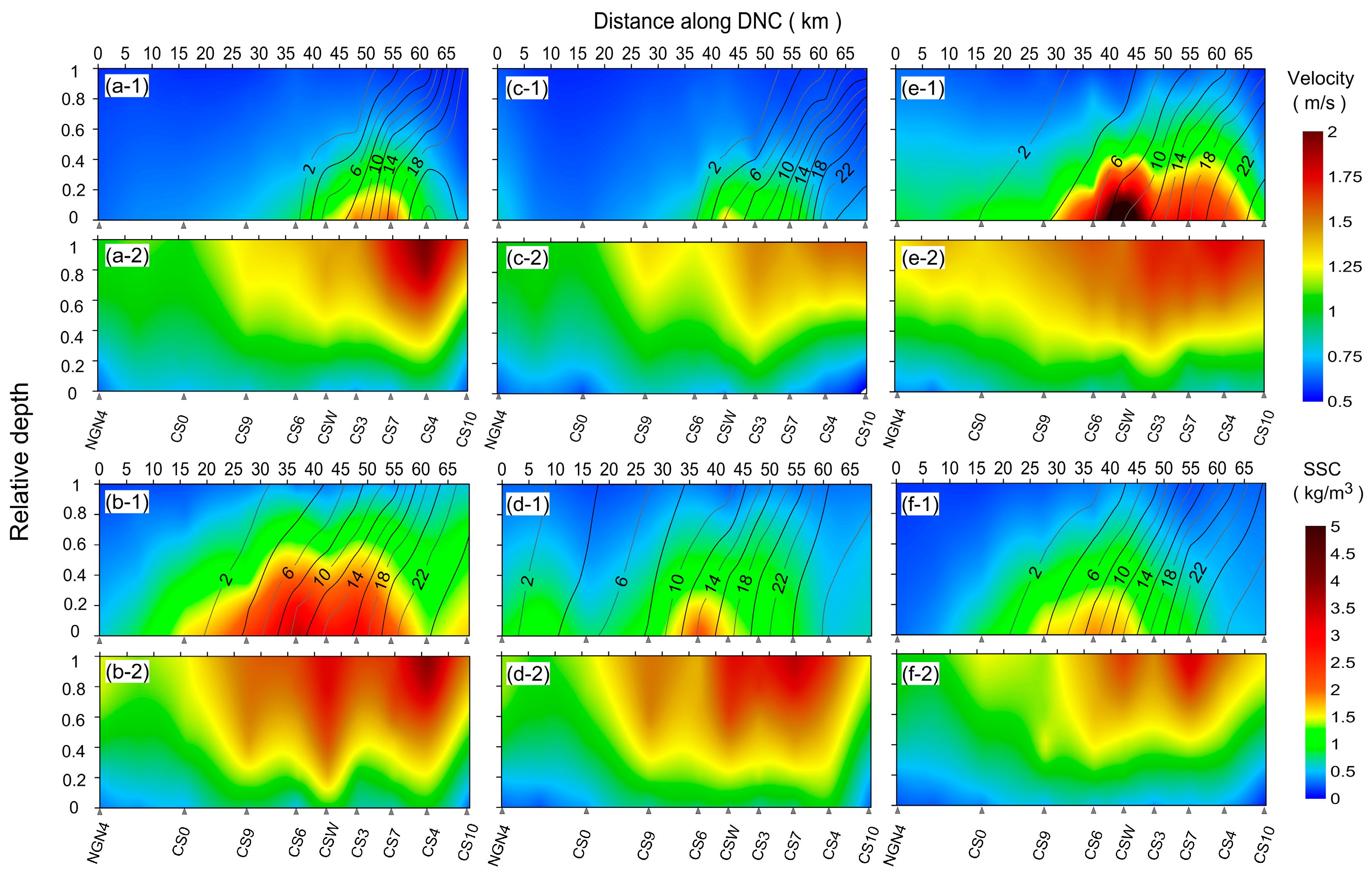
The along-channel profiles of tidal-averaged current velocity, salinity and SSC are shown in Figure 2. The magnitudes of the tidal-averaged current corresponded to the tidal ranges at NPJ (Table 1) and showed a similar pattern of distribution along the DNC in the six observations. The velocities decreased from surface (~1–2 m/s) to bottom (~0.5–1 m/s), with maximum along-channel values in the middle or lower reaches of the DNC (Figure 2(a-2–f-2)). Due to the larger river discharges, the maximum along-channel currents were further downstream in wet seasons. Meanwhile, the length of salinity intrusion (represented by isohalines in Figure 2(a-1–f-1)) was shorter in wet seasons than dry seasons. The most significant salinity intrusion among wet seasons was observed in 2018 (even approaching those in the dry seasons), as a result of a comparatively small discharge, strong tidal dynamic and long-time unchanged SE wind (Figure 2(e-1)).
The SSC increased with water depth and reached the maximum at the bottom in all six observations (Figure 2(a-1–f-1)). The extent of the high SSC (ETM) roughly agreed with the region of salinity intrusion, and the maximum along-channel value located around 10-psu (6–14-psu) isohaline. Therefore, the along-channel distribution of the ETM displayed a similar seasonal variation as the salinity, with a more upstream location in the dry season than the wet season. The ETM was poorly developed with the highest SSC at ~2 kg/m3 and a small extent of high SSC in the wet season but was well developed with the highest SSC at ~3 kg/m3 and a large extent of high SSC in the dry season in 2016 (Figure 2(a-1,b-1)). This phenomenon has been reported and discussed as an abnormal phenomenon in our previous study [25]. Coincidentally, a similar phenomenon was again detected in 2017, with the highest SSC at ~1.5 kg/m3 in the wet season and at ~2.2 kg/m3 in the dry season (Figure 2(c-1,d-1)). In 2018, the SSC was obviously higher in the wet season with the maximum over 5 kg/m3 (in fact, ~8.5 kg/m3) than the dry season with the maximum at ~2 kg/m3 (Figure 2(e-1,f-1)). This remarkable near-bottom high SSC was much higher than those in other observations, even under the similar tidal dynamic (represented by a similar tidal range in NPJ and similar current velocities along the DNC) in the dry season of 2016.
3.2. Inner-Tidal Current, Salinity, Stratification and SSC at Middle DNC
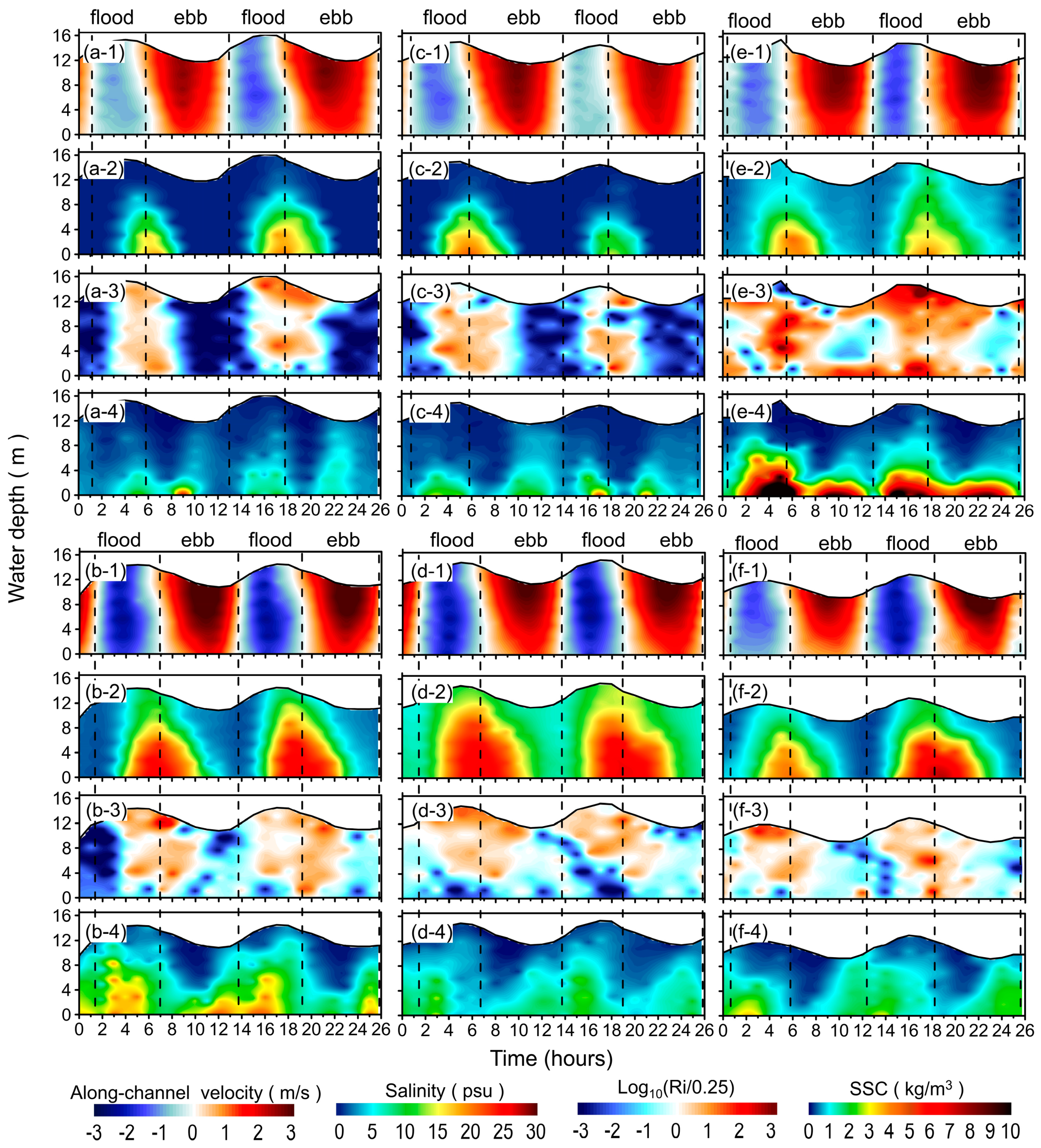
The CSW station located at the middle DNC, where severe siltation exists. The time series of water level, current velocity, salinity and SSC at CSW within two flood-ebb tidal cycles are illustrated. The currents reversed to flood/ebb ~1–2 h after the low/high water level (Figure 3(a-1–f-1)), the phase difference between the current and water level is caused by the combination of friction and channel convergence [39]. The flood and ebb currents showed significant tidal asymmetry in terms of current velocity and duration (represented by time periods between white color bars in Figure 3(a-1–f-1)). Due to the large river discharge and the effect of the DNC project, the ebb currents were much stronger and had longer durations than the flood currents. The durations of flood currents were shorter at the surface than the bottom, while the ebb currents showed the opposite. The vertical asymmetry of the current duration was induced by baroclinic pressure gradient force. This force has the same direction as the flood current and increased with the water depth [15,39]. By the same token, the flood current speeds were more homogeneous along the depth compared with the ebb currents.
The maximum and minimum salinity occurred at high water slack and low water slack, respectively, indicating a movement of saltwater with the flood and ebb currents (Figure 3(a-2–f-2)). In dry seasons, the salinity was higher than the wet season because of a smaller river discharge. The salinity was also related to the tidal dynamic. For example, a stronger salinity intrusion was observed with a larger tidal range in the second tidal cycle than the first in the wet season of 2016 (Figure 3(a-2)).
The stratification and mixing alternated during flood-ebb tidal cycles in six observations (Figure 3(a-3–f-3)), indicated by positive and negative gradient Richardson numbers . The stratification occurred near the high water slack (later flood and early ebb), and the mixing occurred during the rest of the tidal period, in accordance with the advance and retreat of saltwater. The differences of stratification and mixing between wet and dry seasons were not distinct under strong tidal dynamic. In the wet season of 2018, the stratification was stronger than those in other observations and even occurred near the bottom during ebb period (Figure 3(e-3)). Given the similar salinity distribution, the enhanced stratification was more related to weak shear rather than larger buoyancy frequency. In fact, with high SSC near the bottom, the turbulence is significantly inhibited and the weak shear is induced [40,41].
The variation of SSC was more complex than the current, salinity and stratification. Firstly, as mentioned in Section 4.1, the magnitudes of SSC showed a significant difference even in the same season and with similar tidal dynamic. Secondly, although the SSC fluctuated generally with the acceleration and deceleration of the tidal currents, out-of-phase phenomenon between peak SSC and peak flow existed widely, and the peak SSC occurred at different phases during a tidal cycle in six observations (Figure 3(a-4–f-4)). For example, the peak SSC was observed respectively before and after the peak flow during the first flood period in the dry and wet seasons of 2018 (Figure 3(f-4,e-4)). The out-of-phase phenomenon is generally explained by sediments lag [42,43], flow spiral [9] and advection [25].
3.3. Temporal and Spatial Variations of Current, Salinity, Stratification and SSC along the DNC
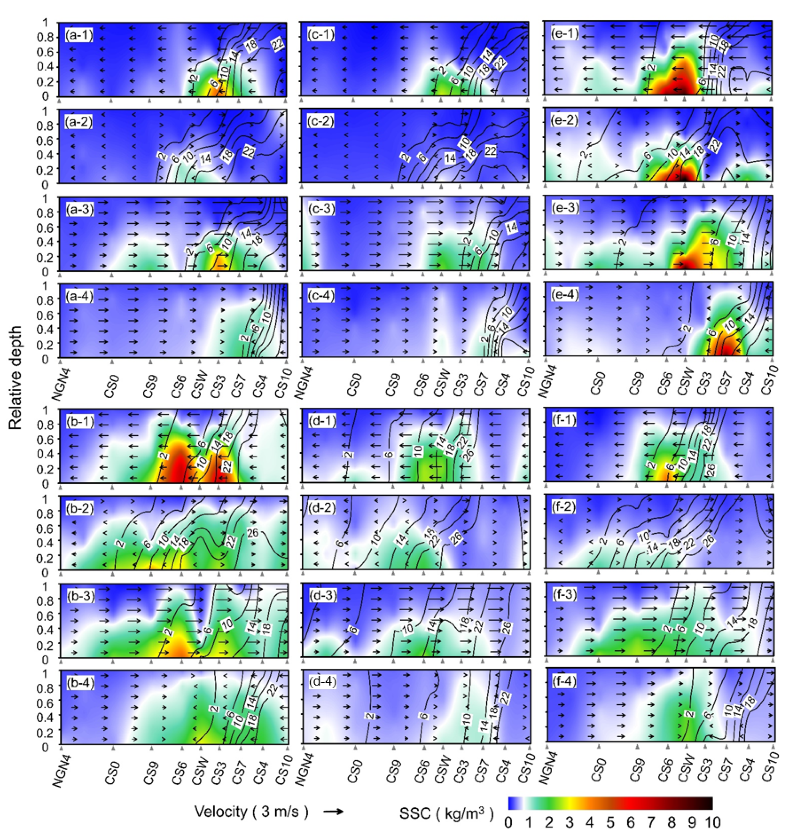
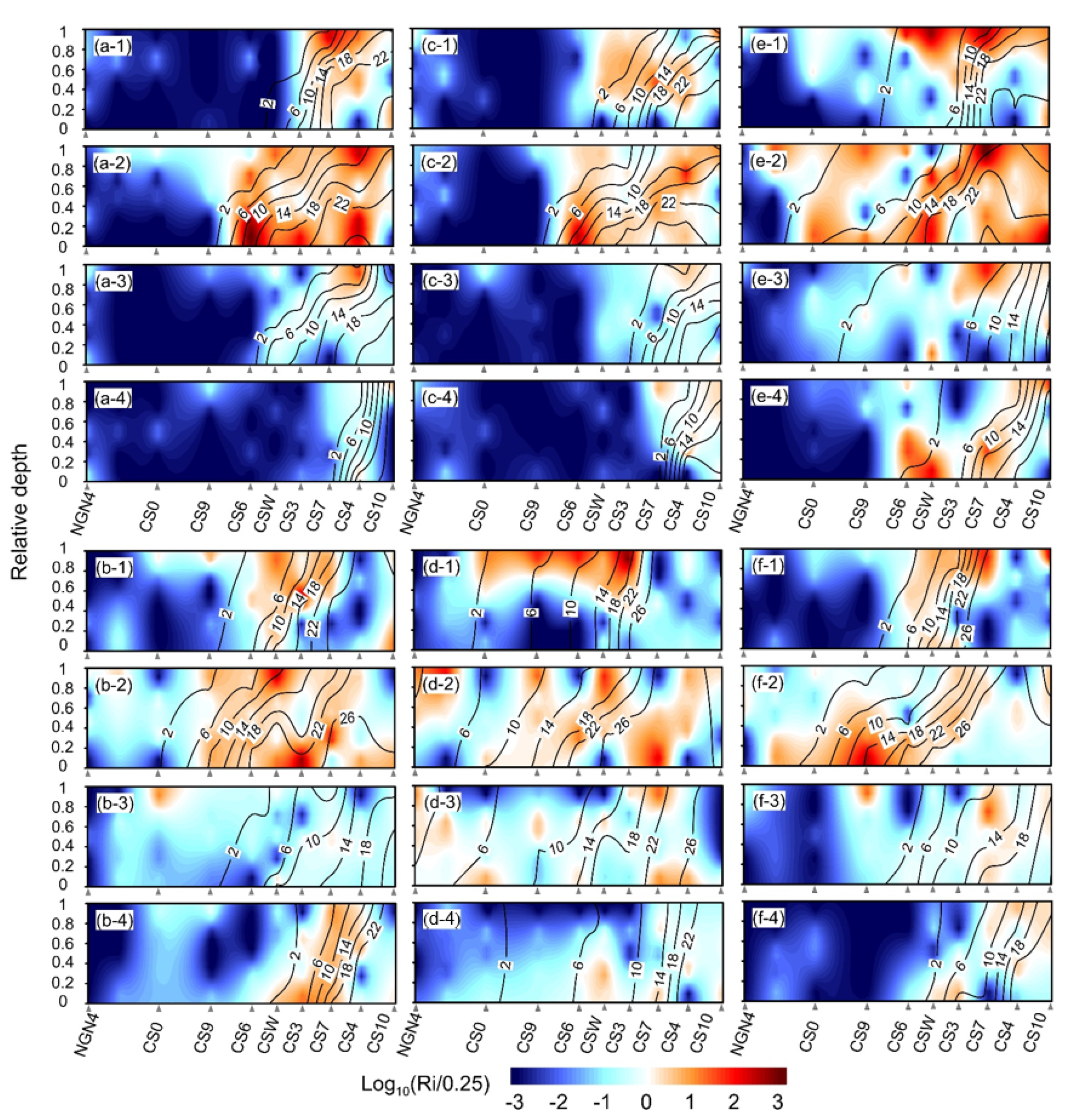
To investigate the temporal and spatial variations of currents, salinity and SSC along the whole DNC, four typical moments (peak flood, high water slack, peak ebb and low water slack) were chosen to show their tidal-varying vertical distributions (Figure 4), and the corresponding mixing and stratification are shown in Figure 5. Due to the interaction between freshwater and saltwater, the currents exhibited a significant along-channel difference. At peak flood and peak ebb, currents in the middle reach were larger than those in the upper and lower reaches (Figure 4(a-1–f-1,a-3–f-3)). At high water slack, the currents reversed to ebb earlier in the upper water column in the lower reach than in the lower water column in the upper reach (Figure 4(a-2–f-2)). At low water slack, the currents reversed to flood earlier at lower water layers in the lower reach than at upper water layers in the upper reach (Figure 4(a-4–f-4)). The isohalines moved upstream and downstream with the flood and ebb currents, and the slopes of isohalines varied during a tidal cycle (Figure 4), inducing alternated mixing and stratification along the DNC (Figure 5). Generally, the stratification was significant at upper and middle water layers at peak flood (Figure 5(a-1–f-1)) and then extended to the upper reach and covered whole water depth at high water slack (Figure 5(a-2–f-2)). During ebb tides, the stratification was weaker than that during flood tide with a smaller vertical salinity gradient (Figure 5(a-3–f-3,a-4–f-4)).
According to previous researches [24,25], a threshold (0.70 kg/m3) of SSC is defined to investigate the extent of the ETM zone (denoted as the white color in Figure 4). Obviously, the ETM zone moved landward and seaward with flooding and ebbing currents, indicating that the effect of advection was important for the motion of ETM in the NP [25]. The along-channel extents of ETM were much larger in dry seasons than those in wet seasons, agreeing well with the intrusion of saltwater. The SSC fluctuated with high values at flood and ebb peaks while with low values at high and low water slacks during most observations. However, the SSC remained a high value at slack water in the wet season of 2018. The most possible reason is due to the hindered settling with high SSC near the bottom [44,45].
3.4. Residual Transport of Water and Sediment
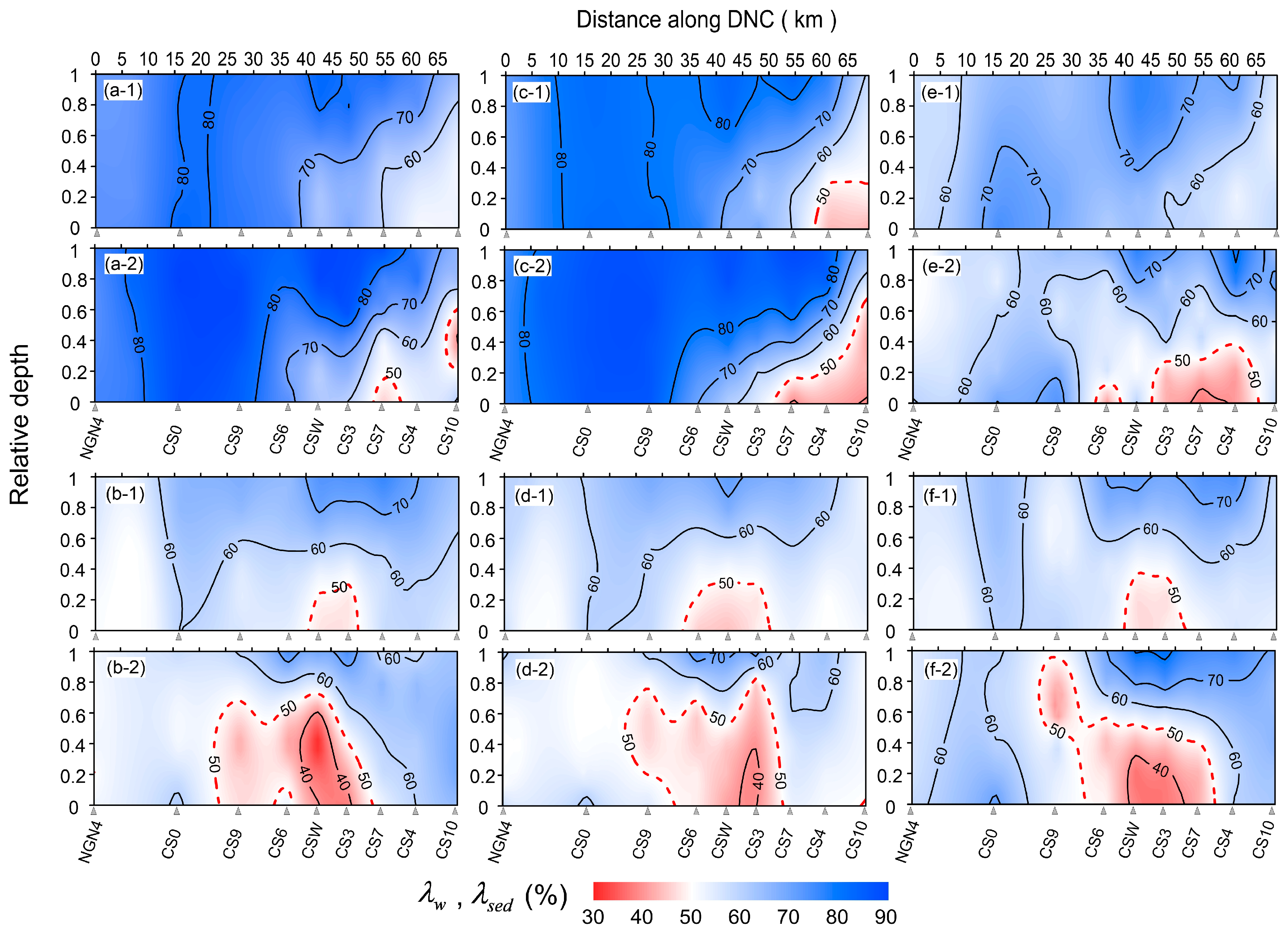
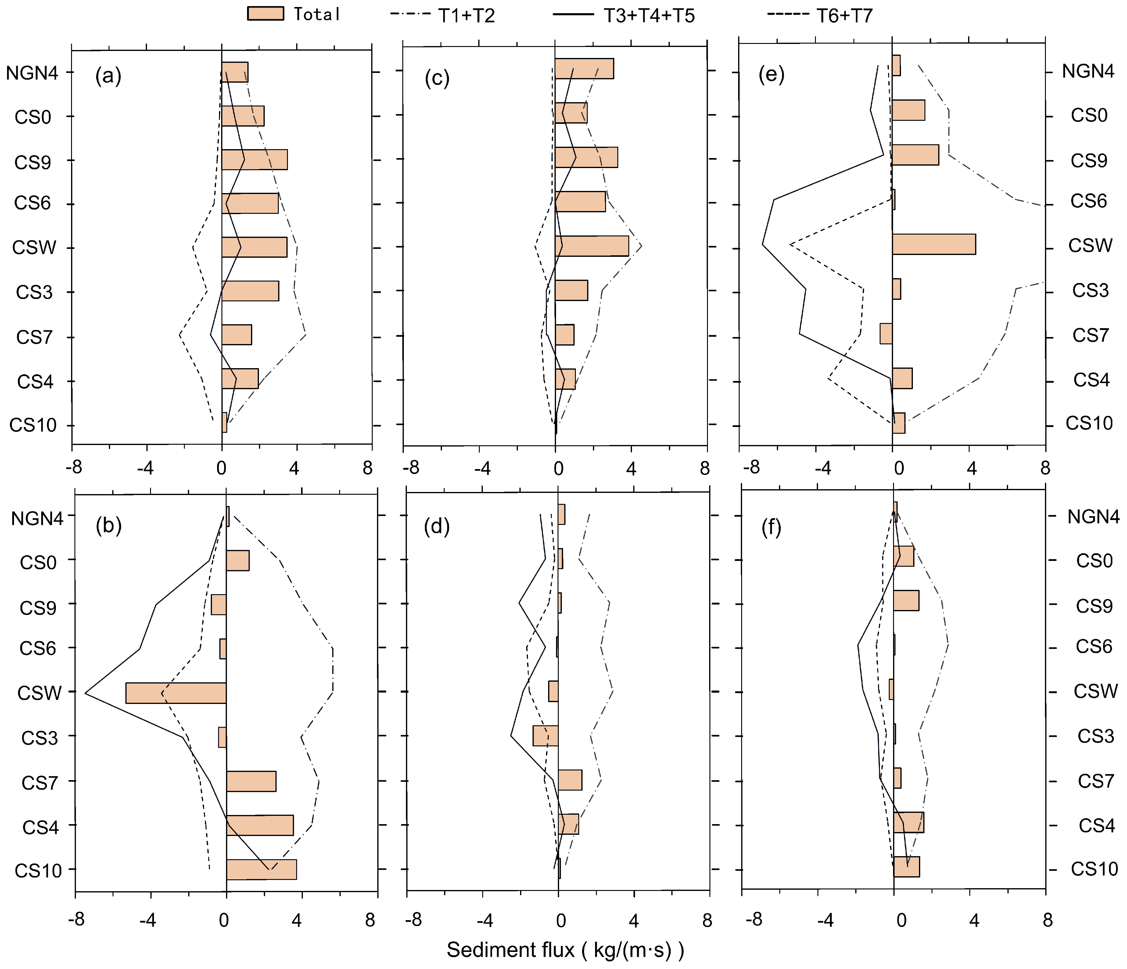
The percentages that ebb water/sediment transport account for the total water/sediment transport ( and ) were calculated using the methods in Section 3.3. In wet seasons, exceeded 50% along the whole channel except seaside stations CS4 and CS10, indicating that the residual water transport was mainly seaward (Figure 6(a-1,c-1,e-1)). The net seaward water transport was induced by large river discharge in this season and by water supply from the south passage [30]. was homogeneous along water depth at landward stations while decreased with depth at seaward stations. This distribution was corresponded well to the distribution of salinity (Figure 2), indicating the significant influence of salt intrusion on residual water transport. In the wet seasons of 2016 and 2017, showed similar distribution as and the residual sediment transport was seaward in the upper and middle reaches (Figure 6(a-2,c-2)). As shown in Figure 7a,c, the advection terms () were all seaward with large magnitudes. The tidal pumping terms () were seaward with relatively small magnitudes at most stations except CS3 and CS7. The vertical circulation terms () were landward, but their magnitudes cannot balance the seaward terms, leading to a seaward transport of the total residual sediment. In the wet season of 2018, despite the seaward residual water transport along the DNC, landward residual sediment transport occurred near the bottom at CS6, CS3, CS7 and CS4 (Figure 6(e-2)). Tidal pumping terms and the vertical gravitation circulation terms are landward, and their magnitudes increased a lot in the middle reach (Figure 7e), resulting in landward residual sediment transport near the bottom in these stations (residual sediment fluxes of the whole water depth were seaward). At CSW, although the landward terms were large, the increase in the seaward advection term was more remarkable, strengthening the seaward residual sediment transport.
In dry seasons, the is generally smaller than that in wet seasons and values < 50% universally occurred in the middle reach in all observations (Figure 6(b-1,d-1,f-1)). With a decrease in river discharge, the domination of ebb water transport receded and the residual water transport turned to landward in the middle reach. Compared to the residual water transport, the landward residual sediment transport in the middle reach was more significant, represented as a larger extent and a smaller magnitude of than (Figure 6(b-2,d-2,f-2)). As shown in Figure 7b,d,f, the tidal pumping and vertical gravitation circulation terms were landward from CS9 to CS7. These landward terms balanced or even overbalanced the seaward advection terms, leading to slight seaward total sediment flux and landward total sediment flux in the middle reach. In the dry season of 2016, the tidal pumping terms near CSW were much larger than those in 2017 and 2018, causing considerable landward residual sediment transport at CSW (Figure 7b).
4. Discussion
4.1. Magnitude of SSC in the ETM Zone
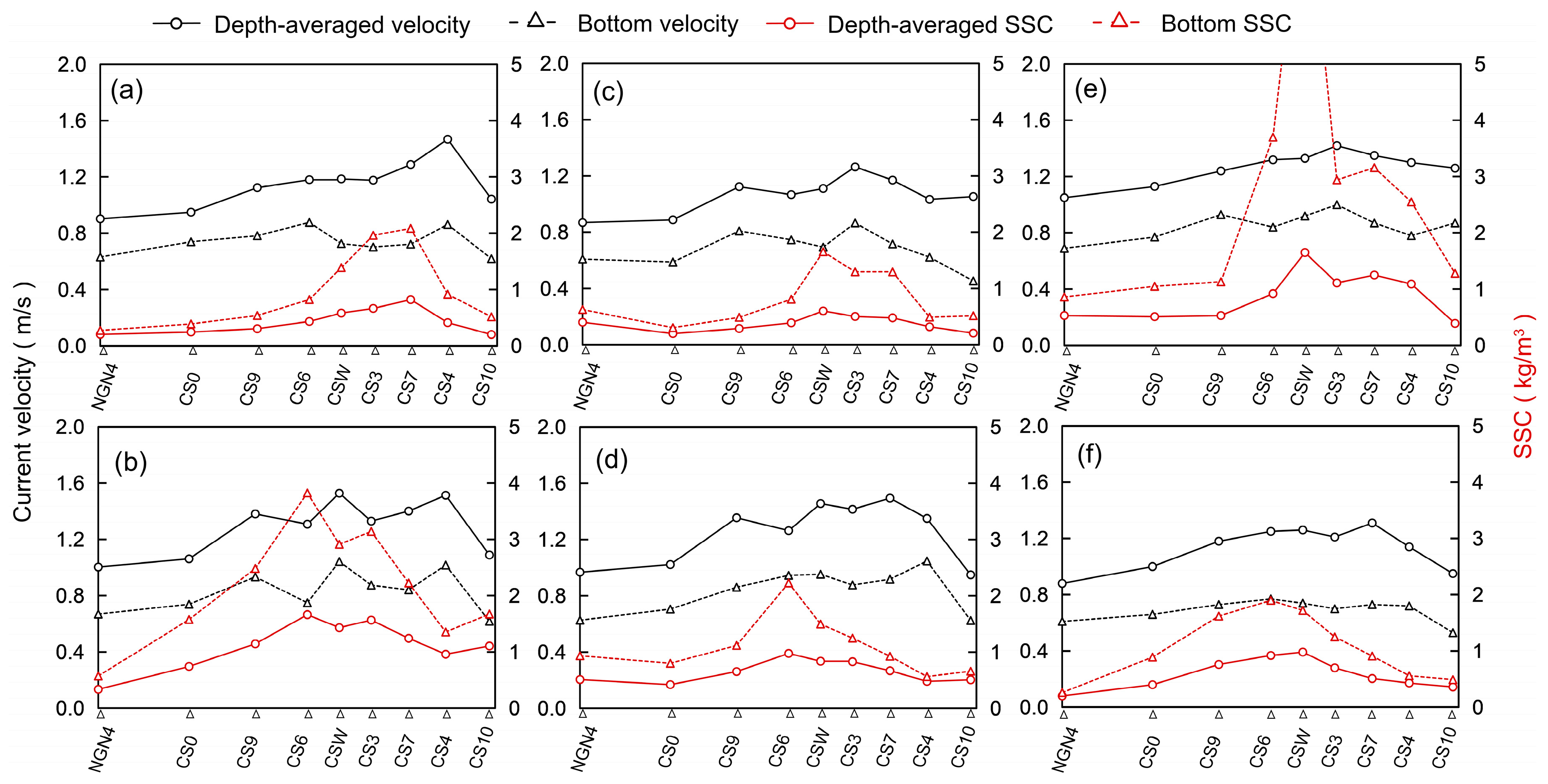
SSC varies not only in flood-ebb tidal cycle but also over the spring-neap tidal cycle [24,26,27], indicating that the magnitude of SSC in the ETM is much related to tidal dynamics. To investigate the influence of tidal dynamics on the magnitude of SSC, the along-channel distribution of the tidal-averaged bottom current velocity and SSC as well as the depth-averaged ones were shown in Figure 8. In the wet season of 2018, the depth-averaged current velocity of all the observation stations was ~1.1/1.2 times as large as those in the wet seasons of 2016 and 2017, while the depth-averaged SSC showed ~2.1/2.4 times differences (Figure 8a,c,e). At the bottom, a slight increase in velocity led to a more significant increase in SSC, with ~2.8/3.4 times difference in all stations and ~6.2/5.2 times difference in CSW. The tidal dynamics were similar in dry seasons of 2016 and 2017, while the magnitudes of SSC in 2016 were ~1.7/2 times higher in the bottom layer/all water depth than those in 2017. Moreover, the tidal dynamics in 2017 were stronger than 2018 but the SSC showed little differences. Hence, the magnitude of SSC was more than determined by tidal dynamics, indicating that other controlling factors existed.
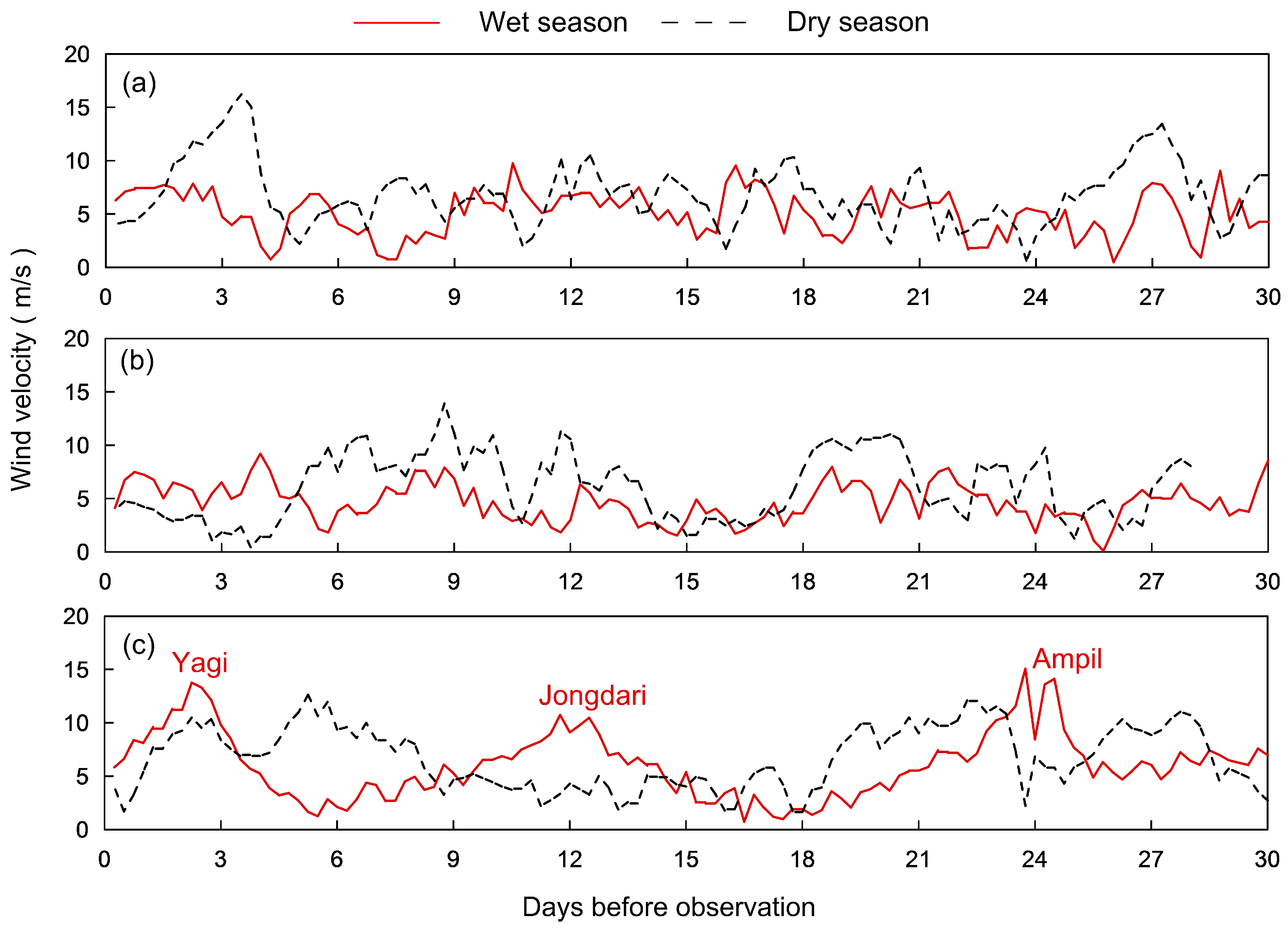
In our previous study, we have proposed that the magnitude of SSC in the ETM is not only affected by tidal dynamic but also by the quantity of sediments available to resuspend, which was related to extreme weather before the observation [25]. This opinion was examined by all observations in this new study. Lacking on-site wind and wave data before observations, we used wind data near the NPJ station from the European Center for Medium-Range Weather Forecasts (ECMWF) (Figure 9). In the wet seasons of 2016 and 2017, the wind speeds before observations were relatively stable with modest magnitudes, indicating that typhoons had weak influences on the CRE. As a result, the SSC was relatively low with insufficient sediment available to resuspend here. The weak resuspension effects were identified by small tidal pumping terms in these two observations (Figure 7a,c), given that tidal pumping terms indicate the exchange of sediments between water and stream bed under the tidal dynamics [5]. On the contrary, three typhoons influenced the CRE and induced strong winds before the observation in the wet season of 2018. Particularly, the typhoon “Yagi” passed by the CRE just two days before the observation. In the dry season of 2016, a strong cold-air front occurred with strong winds three days before the observation. Therefore, the SSC in these two observations was significantly higher than other observations because of sufficient sediment available to resuspend, identified by large tidal pumping terms (Figure 7b,e). Moreover, the winds in 2017 were smaller than those in 2018 six days before the observations. Therefore, the stronger tidal dynamic in 2017 than 2018 failed to induce an obvious increase in SSC because of less sediment available to resuspend. We once considered the “reversed” seasonal variation of SSC in 2016 as an abnormal phenomenon [25]. Based on the multi-year observations, this “reversed” seasonal variation of SSC was again detected in 2017. Hence, the common perspective that SSC is higher in the wet season than the dry season seems a bit of arbitrary, considering that the magnitudes of SSC were easily influence by strong winds during all observations. The influence of winds, especially strong winds on suspended sediment, are reported in many other estuaries, such as the Jiulong River Estuary (China) [46], the Mandovi Estuary (India) [47,48], the Tay Estuary (UK) [49] and the Tavy estuary (UK) [50]. In the Mandovi Estuary [47,48], winds are even the major formation mechanism of the ETM. The influences of winds on suspended sediment originate from the enhanced resuspension induced by wind-driven waves [51]. Then, the influences differ a lot among estuaries because of the different dynamics and topographies. Based on our previous study [25] and some other studies [28,29], the cross-dike sediment transport from the JDS to the NP is enhanced by stronger resuspension on the shoal and a higher water level near the dikes under strong winds. Then, the large amount of sediments was trapped in the NP (possibly in the form of fluid mud) and influenced the magnitudes of SSC by current-dominated resuspension. However, as mentioned in Section 2.1, the dynamics and topography are so complex in the CRE and it is still unclear if sediments come from other regions (such as outer sea or regions between dikes) under strong winds. Hence, more importance should be attached to the influence of winds on sediment transport in the CRE, especially in the NP.
4.2. Along-Channel and Vertical Distribution of SSC in the ETM Zone
The high SSC moved upstream and downstream with the advance and retreat of isohalines during the flood-ebb cycle (Figure 4). The extent of the tidal-averaged high SSC roughly coincided with the region of salinity intrusion, with the maximum value locating around 10-psu isohaline (Figure 2(a-1–f-1)), but showed a weak relationship with the along-channel current (Figure 2(a-2–f-2) and Figure 8). This meant that the along-channel distribution of SSC was determined well by the along-channel location of the salt wedge, and thus, the ETM was further upstream in the dry season than the wet season.
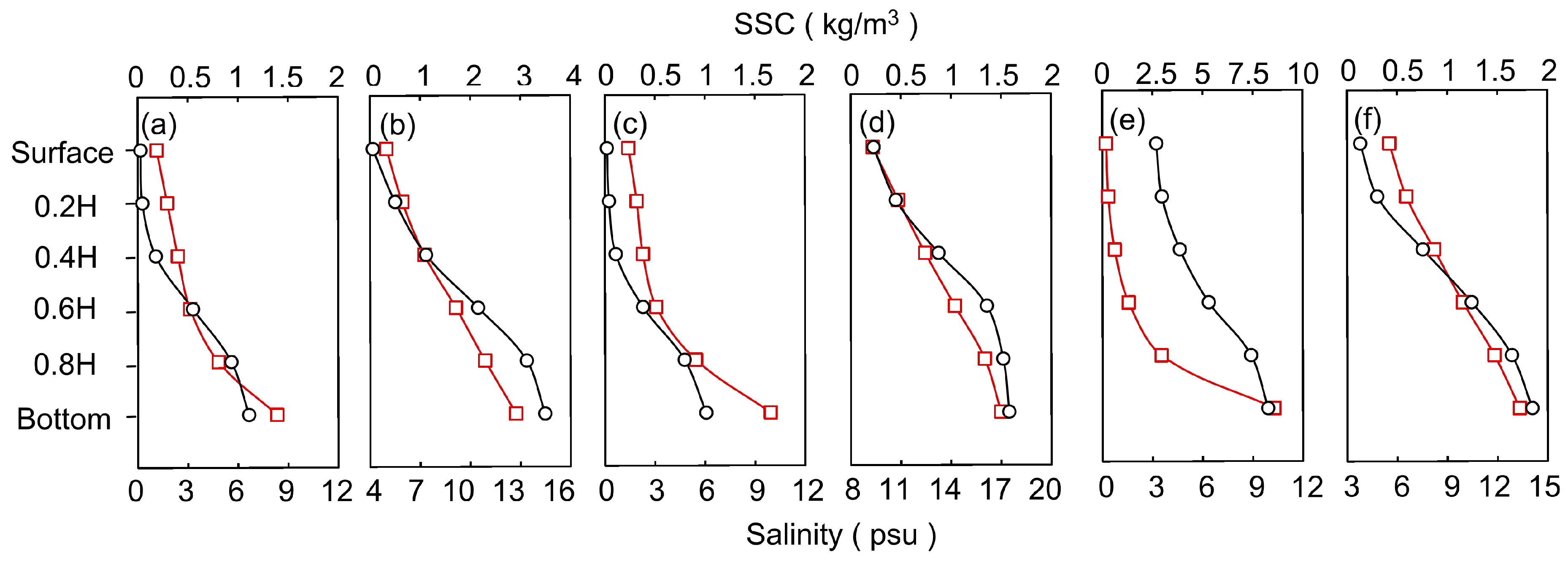
Li et al. [52] categorizes instantaneous vertical profiles of SSC into three types in the NP. In fact, the instantaneous profiles of SSC are more complex and irregular, while tidal-averaged profiles of SSC were regularly exponential [53]. Hence, the tidal-averaged profiles were used to investigate the vertical distribution of SSC in this study (Figure 10). The tidal-averaged SSC and salinity increased with the water depth. Compared to dry seasons, the salinity showed a steeper slope along the depth with a smaller difference between surface and bottom in wet seasons, indicating a weaker tidal-averaged stratification. The vertical profiles of SSC were in “‘exponential” style in the wet seasons while in “linear” style in the dry season. This meant that the high SSC was more concentrated in lower water layers in wet seasons. The vertical distribution of SSC is often reported to be influenced by stratification [15,21,52]. The more concentrated SSC in lower water layers occurred in environment with weaker stratification; thus, stratification was not the reason for this seasonal difference of vertical SSC. As reported by Wan et al. [54], the flocculation setting velocity increased with rise in temperature, especially under a high-SSC condition. Hence, more concentrated SSC in lower water layers was induced by a larger setting velocity in wet seasons and the concentrated SSC was most distinct in the wet season of 2018, with the highest SSC among the three years. Of course, the vertical distribution of SSC dominated by the flocculation setting was for the spring tides with weak stratification. During middle and neap tides when the stratification is enhanced, further researches are required to reappraise the contributions of flocculation setting and stratification to the vertical SSC.
4.3. Sediment Transport and Siltation in the DNC
In previous studies, the convergences of residual sediment flux in the middle DNC are widely observed [14,15,20,38]. Most of them are based on a single observation and are used to explain sediment trapping and siltation in this reach [14,20,38]. Li et al. [15] point out that the sediment transport and convergences vary within a spring-neap tidal cycle while the concern about seasonal difference of sediment transport and convergence is still lacking. Based on multi-year observations in both the wet and dry seasons, the water and sediment transports showed distinct seasonal differences in our research. The residual water and sediment fluxes in lower water layers were landward in the middle reach of the DNC in dry seasons (Figure 6b,d,f). The landward sediment fluxes converged with those seaward fluxes from the upper reach, inducing sediment trapping and siltation in the seaward segment of the upper reach (Figure 6(b-2,d-2,f-2)). However, due to the large river discharges, the residual water fluxes were seaward in the middle reach in wet seasons (Figure 6(a-1,c-1,e-1)). In the wet seasons in 2016 and 2017 when the SSC was relatively low, the advection effect dominated (Figure 7a,c); thus, the residual sediment fluxes were seaward, corresponding to the residual water fluxes (Figure 6(a-2,c-2)). The absence of convergent residual water and sediment flux was not conducive to sediment trapping and siltation in the middle reach (convergence occurred in the lower reach). In the wet season of 2018 when the SSC was relatively high, the enhanced tidal pumping effect (Figure 7e) induced landward residual sediment fluxes at CS6 and CS3 near the bottom (the residual sediment fluxes of the whole water depth were seaward), and a near-bottom convergence occurred between CSW and CS3 favouring the siltation (Figure 6(e-2)).
Compared to 2011–2015, siltation in the middle DNC reduced in 2016 and 2017; Liu et al. [55] infer that the low SSC and reduced siltation are mainly owing to the increase in the height of the sediment-preventing dike from 2015 to early 2016 and partly due to the weaker influence of typhoon. The recovery of high SSC in 2018 explained that the increase in the height of sediment-preventing dikes was not the crucial reason for low SSC in 2016 and 2017. Based on our research, the low SSC was mainly related to the weaker influence of typhoons. Moreover, the large river discharge and a low-SSC condition jointly limited the siltation in the middle reach. The former vanished convergence of water flux, and the later reduced landward tidal pumping effect.
5. Conclusions
To investigate more general features and mechanisms of ETM in the NP, multi-year observations were conducted in 2016, 2017 and 2018. The ETM showed different seasonal variations among the three years: the SSC was lower in wet seasons than dry seasons in 2016 and 2017 while higher in the wet season than the dry season in 2018. The common perspective that SSC is higher in wet seasons than dry seasons seemed a bit of arbitrary, and the winds before observations played an important role on the magnitude of SSC besides the tidal dynamic.
The extent of the tidal-averaged high SSC roughly coincided with the intrusion region of salinity, and the along-channel maximum value was approximately located around 10-psu isohaline. Under strong tidal dynamics, there were small differences in stratification between wet and dry seasons and tidal-averaged stratification was slightly weaker in wet seasons. The SSC showed “exponential” profiles in wet seasons but “linear” profiles in dry seasons, indicating that the high SSC was more concentrated in lower water layers in wet seasons. The more concentrated high SSC in lower water layers in wet seasons was induced by a larger setting velocity under higher water temperatures rather than the weaker stratification.
The large river discharge vanished convergence of water transport, and the low-SSC condition reduced the landward tidal pumping effect during spring tides in the wet seasons of 2016 and 2017, jointly limiting the siltation in the middle DNC. Compared to wet seasons, sediment trapping and siltation in the dry seasons occurred in the seaward segment of the upper reach because of a decrease in the river discharge.
Author Contributions
H.H. and Y.W. conceived this study, and collected the data; X.H. analyzed the data and results; X.Y., K.Z. and D.C. participated in the discussion of the results; All authors contributed to the preparation of this manuscript. All authors have read and agreed to the published version of the manuscript.
Funding
This research was funded by National Key R&D Program of China (2017YFC0405401), National Natural Science Foundation of China (51979096), Fundamental Research Funds for the Central Universities (2018B636X14) and by the Postgraduate Research & Practice Innovation Program of Jiangsu Province (KYCX18_0603).
Acknowledgments
This work was supported by the National Key R&D Program of China (2017YFC0405401), by the National Natural Science Foundation of China (51979096), by the Fundamental Research Funds for the Central Universities (2018B636X14) and by the Postgraduate Research & Practice Innovation Program of Jiangsu Province (KYCX18_0603). We also acknowledge the anonymous reviewers for their valuable comments and suggestions.
Conflicts of Interest
The authors declare no conflict of interest.
References
- Burchard, H.; Schuttelaars, H.M.; Ralston, D.K. Sediment trapping in estuaries. Annu. Rev. Mar. Sci. 2018, 10, 371–395. [Google Scholar] [CrossRef] [PubMed]
- Festa, J.F.; Hansen, D.V. Turbidity maxima in partially mixed estuaries: A two-dimensional numerical model. Estuar. Coast. Mar. Sci. 1978, 7, 347–359. [Google Scholar] [CrossRef]
- Jay, D.A.; Smith, J.D. Residual circulation in shallow estuaries: 1. Highly stratified, narrow estuaries. J. Geophys. Res. Ocean. 1990, 95, 711–731. [Google Scholar] [CrossRef]
- Allen, G.; Salomon, J.; Bassoullet, P.; Du Penhoat, Y.; De Grandpre, C. Effects of tides on mixing and suspended sediment transport in macrotidal estuaries. Sediment. Geol. 1980, 26, 69–90. [Google Scholar] [CrossRef]
- Dyer, K.R. Fine sediment particle transport in estuaries. In Physical Process in Estuaries; Dronkers, J., van Leussen, W., Eds.; Springer: Berlin, Germany, 1988. [Google Scholar]
- Gallenne, B. Study of fine material in suspension in the estuary of the loire and its dynamic grading. Estuar. Coast. Mar. Sci. 1974, 2, 261–272. [Google Scholar] [CrossRef]
- Geyer, W.R. The importance of suppression of turbulence by stratification on the estuarine turbidity maximum. Estuaries 1993, 16, 113–125. [Google Scholar] [CrossRef]
- Scully, M.E.; Friedrichs, C.T. The influence of asymmetries in overlying stratification on near-bed turbulence and sediment suspension in a partially mixed estuary. Ocean Dyn. 2003, 53, 208–219. [Google Scholar] [CrossRef]
- Wu, J.; Liu, J.T.; Wang, X. Sediment trapping of turbidity maxima in the changjiang estuary. Mar. Geol. 2012, 303–306, 14–25. [Google Scholar] [CrossRef]
- Wolanski, E.; Gibbs, R.J. Flocculation of suspended sediment in the Fly River Estuary, Papua New Guinea. J. Coast. Res. 1995, 11, 754–762. [Google Scholar]
- Shi, J.Z.; Lu, L.-F. A short note on the dispersion, mixing, stratification and circulation within the plume of the partially-mixed changjiang river estuary, China. J. Hydro-Environ. Res. 2011, 5, 111–126. [Google Scholar] [CrossRef]
- Chernetsky, A.S.; Schuttelaars, H.M.; Talke, S.A. The effect of tidal asymmetry and temporal settling lag on sediment trapping in tidal estuaries. Ocean Dyn. 2010, 60, 1219–1241. [Google Scholar] [CrossRef] [Green Version]
- Geyer, W.R.; Woodruff, J.D.; Traykovski, P. Sediment transport and trapping in the hudson river estuary. Estuaries 2001, 24, 670–679. [Google Scholar] [CrossRef]
- Liu, G.; Zhu, J.; Wang, Y.; Wu, H.; Wu, J. Tripod measured residual currents and sediment flux: Impacts on the silting of the deepwater navigation channel in the changjiang estuary. Estuar. Coast. Shelf Sci. 2011, 93, 192–201. [Google Scholar] [CrossRef]
- Li, X.; Zhu, J.; Yuan, R.; Qiu, C.; Wu, H. Sediment trapping in the changjiang estuary: Observations in the north passage over a spring-neap tidal cycle. Estuar. Coast. Shelf Sci. 2016, 177, 8–19. [Google Scholar] [CrossRef]
- Shen, Q.; Huang, W.; Wan, Y.; Gu, F.; Qi, D. Observation of the sediment trapping during flood season in the deep-water navigational channel of the changjiang estuary, China. Estuar. Coast. Shelf Sci. 2020, 237, 106632. [Google Scholar] [CrossRef]
- Pu, X.; Shi, J.Z.; Hu, G.-D.; Xiong, L.-B. Circulation and mixing along the north passage in the changjiang river estuary, China. J. Mar. Syst. 2015, 148, 213–235. [Google Scholar] [CrossRef]
- Li, J.; Zhang, C. Sediment resuspension and implications for turbidity maximum in the changjiang estuary. Mar. Geol. 1998, 148, 117–124. [Google Scholar] [CrossRef]
- Li, L.; Wu, H.; Liu, J.T.; Zhu, J. Sediment transport induced by the advection of a moving salt wedge in the changjiang estuary. J. Coast. Res. 2015, 31, 671–679. [Google Scholar] [CrossRef]
- Wan, Y.; Zhao, D. Observation of saltwater intrusion and etm dynamics in a stably stratified estuary: The yangtze estuary, china. Environ. Monit. Assess. 2017, 189, 89. [Google Scholar] [CrossRef]
- Song, D.; Wang, X.; Cao, Z.; Guan, W. Suspended sediment transport in the deepwater navigation channel, yangtze river estuary, china, in the dry season 2009: 1. Observations over spring and neap tidal cycles. J. Geophys. Res. Ocean. 2013, 118, 5555–5567. [Google Scholar] [CrossRef]
- Shen, H.; Zhu, H.; Mao, Z. Circulation of the chang jiang estuary and its effect on the transport of suspended sediment. In Estuarine Comparisons; Kennedy, V.S., Ed.; Academic Press: London, UK, 1982; pp. 677–691. [Google Scholar]
- Chen, S.-L.; Zhang, G.-A.; Yang, S.-L.; Shi, J.Z. Temporal variations of fine suspended sediment concentration in the changjiang river estuary and adjacent coastal waters, china. J. Hydrol. 2006, 331, 137–145. [Google Scholar] [CrossRef]
- Yang, Y.; Li, Y.; Sun, Z.; Fan, Y. Suspended sediment load in the turbidity maximum zone at the yangtze river estuary: The trends and causes. J. Geogr. Sci. 2014, 24, 129–142. [Google Scholar] [CrossRef]
- Hua, X.; Huang, H.; Wang, Y.; Lan, Y.; Zhao, K.; Chen, D. Abnormal etm in the north passage of the changjiang river estuary: Observations in the wet and dry seasons of 2016. Estuar. Coast. Shelf Sci. 2019, 227, 106334. [Google Scholar] [CrossRef]
- Shen, H.; Pan, D. Turbidity Maximum in the Changjiang Estuary; China Ocean: Beijing, China, 2001. [Google Scholar]
- Wan, Y.; Wang, L. Study on the seasonal estuarine turbidity maximum variations of the yangtze estuary, china. J. Waterw. Port Coast. Ocean Eng. 2018, 144, 05018002. [Google Scholar] [CrossRef]
- Wan, Y.; Roelvink, D.; Li, W.; Qi, D.; Gu, F. Observation and modeling of the storm-induced fluid mud dynamics in a muddy-estuarine navigational channel. Geomorphology 2014, 217, 23–36. [Google Scholar] [CrossRef]
- Shen, Q.; Huang, W.; Qi, D. Integrated modeling of typhoon damrey’s effects on sediment resuspension and transport in the north passage of changjiang estuary, china. J. Waterw. Port Coast. Ocean Eng. 2018, 144, 04018015. [Google Scholar] [CrossRef]
- Wu, H.; Zhu, J.; Choi, B.H. Links between saltwater intrusion and subtidal circulation in the changjiang estuary: A model-guided study. Cont. Shelf Res. 2010, 30, 1891–1905. [Google Scholar] [CrossRef]
- Liu, J.; Zhao, D.Z.; Cheng, H.F. Recent morphological evolution of Jiuduan shoal and its effect on navigation channel sedimentation of north passage in Yangtze River Estuary. J. Yangtze River Sci. Res. Inst. 2010, 27, 1–5. [Google Scholar]
- Hu, K.; Ding, P. The effect of deep waterway constructions on hydrodynamics and salinities in Yangtze Estuary, china. J. Coast. Res. 2009, 2, 961–965. [Google Scholar]
- Wang, Y.; Shen, J.; He, Q. A numerical model study of the transport timescale and change of estuarine circulation due to waterway constructions in the Changjiang Estuary, China. J. Mar. Syst. 2010, 82, 154–170. [Google Scholar] [CrossRef]
- Jiang, C.; de Swart, H.E.; Li, J.; Liu, G. Mechanisms of along-channel sediment transport in the north passage of the yangtze estuary and their response to large-scale interventions. Ocean Dyn. 2013, 63, 283–305. [Google Scholar] [CrossRef]
- Changjiang River Sediment Bulletin. Available online: http://www.cjw.gov.cn/zwzc/bmgb/ (accessed on 26 April 2019).
- Schlichting, H. Hauptaufsätze. Turbulenz bei wärmeschichtung. ZAMM-J. Appl. Math. Mech./Zeitschrift Für Angewandte Mathematik Und Mechanik 1935, 15, 313–338. [Google Scholar] [CrossRef]
- Stacey, M.; Rippeth, T.; Nash, J. Turbulence and Stratification in Estuaries and Coastal Seas. In Treatise on Estuarine and Coastal Science; McLusky, D., Wolanski, E., Eds.; Elsevier: Amsterdam, The Netherlands, 2011; Volume 2, pp. 9–35. [Google Scholar]
- Li, L.; He, Z.; Xia, Y.; Dou, X. Dynamics of sediment transport and stratification in changjiang river estuary, china. Estuar. Coast. Shelf Sci. 2018, 213, 1–17. [Google Scholar] [CrossRef]
- Jay, D.A.; Musiak, J.D. Internal tidal asymmetry in channel flows: Origins and consequences. In Mixing Processes in Estuaries and Coastal Seas; Pattiaratchi, C., Ed.; American Geophysical Union: Washington, DC, USA, 1996; pp. 211–249. [Google Scholar]
- Cloutier, D.; LeCouturier, M.N.; Amos, C.L.; Hill, P.R. The effects of suspended sediment concentration on turbulence in an annular flume. Aquat. Ecol. 2006, 40, 555–565. [Google Scholar] [CrossRef]
- Sheng, Y.P.; Villaret, C. Modeling the effect of suspended sediment stratification on bottom exchange processes. J. Geophys. Res. Ocean. 1989, 94, 14429–14444. [Google Scholar] [CrossRef]
- Van Kessel, T.; Vanlede, J.; de Kok, J. Development of a mud transport model for the scheldt estuary. Cont. Shelf Res. 2011, 31, S165–S181. [Google Scholar] [CrossRef] [Green Version]
- Yu, Q.; Flemming, B.W.; Gao, S. Tide-induced vertical suspended sediment concentration profiles: Phase lag and amplitude attenuation. Ocean Dyn. 2011, 61, 403–410. [Google Scholar] [CrossRef]
- Winterwerp, J.C.; Van Kesteren, W.G. Introduction to the Physics of Cohesive Sediment Dynamics in the Marine Environment; Elsevier: Amsterdam, The Netherlands, 2004. [Google Scholar]
- Dankers, P.J.T.; Winterwerp, J.C. Hindered settling of mud flocs: Theory and validation. Cont. Shelf Res. 2007, 27, 1893–1907. [Google Scholar] [CrossRef]
- Chen, N.; Krom, M.D.; Wu, Y.; Yu, D.; Hong, H. Storm induced estuarine turbidity maxima and controls on nutrient fluxes across river-estuary-coast continuum. Sci. Total Environ. 2018, 628, 1108–1120. [Google Scholar] [CrossRef] [PubMed]
- Rao, V.P.; Shynu, R.; Kessarkar, P.M.; Sundar, D.; Michael, G.S.; Narvekar, T.; Blossom, V.; Mehra, P. Suspended sediment dynamics on a seasonal scale in the mandovi and zuari estuaries, central west coast of india. Estuar. Coast. Shelf Sci. 2011, 91, 78–86. [Google Scholar]
- Kessarkar, P.M.; Rao, V.P.; Shynu, R.; Ahmad, I.M.; Mehra, P.; Michael, G.S.; Sundar, D. Wind-driven estuarine turbidity maxima in mandovi estuary, central west coast of india. J. Earth Syst. Sci. 2009, 118, 369–377. [Google Scholar] [CrossRef] [Green Version]
- Weir, D.J.; Mcmanus, J. The role of wind in generating turbidity maxima in the tay estuary. Cont. Shelf Res. 1987, 7, 1315–1318. [Google Scholar] [CrossRef]
- Uncles, R.J.; Stephens, J. Turbidity and sediment transport in a muddy sub-estuary. Estuar. Coast. Shelf Sci. 2010, 87, 213–224. [Google Scholar] [CrossRef]
- Green, M.; Coco, G. Review of wave-driven sediment resuspension and transport in estuaries. Rev. Geophys. 2014, 52, 77–117. [Google Scholar] [CrossRef]
- Li, Z.; Jia, J.; Wu, Y.; Zong, H.; Zhang, G.; Wang, Y.P.; Yang, Y.; Zhou, L.; Gao, S. Vertical distributions of suspended sediment concentrations in the turbidity maximum zone of the periodically and partially stratified changjiang estuary. Estuaries Coasts 2019, 42, 1475–1490. [Google Scholar] [CrossRef]
- Liu, J.; Yang, S.; Zhu, Q.; Zhang, J. Controls on suspended sediment concentration profiles in the shallow and turbid yangtze estuary. Cont. Shelf Res. 2014, 90, 96–108. [Google Scholar] [CrossRef]
- Wan, Y.; Wu, H.; Roelvink, D.; Gu, F. Experimental study on fall velocity of fine sediment in the yangtze estuary, china. Ocean Eng. 2015, 103, 180–187. [Google Scholar] [CrossRef]
- Liu, J.; Cheng, H.; Han, L.; Wang, Z. Interannual variations on siltation of the 12. 5 m deepwater navigation channel in Yangtze Estuary. Adv. Water Sci. 2019, 30, 65–75. [Google Scholar]
Figure 1.
(a) Location of the Changjiang River Estuary and Datong gauge station, (b) topography of the Changjiang River Estuary (refer to the 85 National Vertical Datum of China), and (c) the location of observation stations and the Deepwater Navigation Channel (DNC) project (upper reach: NGN4–CS9, middle reach: CS6–CS3, and lower reach: CS7–CS10).

Figure 2.
Along-channel distributions of tidal-averaged current velocity magnitude, salinity and suspended sediment concentration (SSC): (a–f) represent the wet and dry seasons of 2016, wet and dry seasons of 2017, and wet and dry seasons of 2018 respectively. (1)—SSC and isohalines (with the interval of 2 psu) and (2)—magnitude of tidal-averaged current velocity (calculated by absolute values of current velocities during two flood-ebb tidal cycle and denoting the strength of tidal dynamic).

Figure 3.
Variations of along-channel current, salinity, stratification and SSC during two flood-ebb tidal cycles at CSW: (a–f) represent six observations respectively (according to Figure 2). (1–4) represent along-channel current velocity, salinity, gradient Richardson number and SSC, respectively. Positive velocity denotes seaward current, and negative velocity denotes landward current.

Figure 4.
Variations of axial current, salinity and SSC along the DNC: The (a–f) represent six observations, respectively (according to Figure 2). (1–4) represent peak flood, high water slack, peak ebb and low water, slack respectively. The rightward arrow means seaward axial current, and the leftward arrow means landward axial current. The isohalines (in psu) are shown in black lines.

Figure 5.
Variations of salinity and stratification along the DNC: The (a–f) represent six observations, respectively (according to Figure 2). (1–4) represent peak flood, high water slack, peak ebb and low water slack, respectively. The isohalines (in psu) are shown in black lines.
Figure 5.
Variations of salinity and stratification along the DNC: The (a–f) represent six observations, respectively (according to Figure 2). (1–4) represent peak flood, high water slack, peak ebb and low water slack, respectively. The isohalines (in psu) are shown in black lines.

Figure 6.
Percentages that ebb water/sediment transport account for the total water/sediment transport along the DNC: (a–f) represent six observations, respectively (according to Figure 2). (1)—and (2)—represent water transport and sediment transport , respectively. The red dashed lines represent the value 50%. Values >50% denotes ebb-dominated and seaward residual transport, while values <50% denote flood-dominated and landward residual transport.

Figure 7.
Components of total sediment fluxes at along-channel stations: The (a–f) represent six observations, respectively (according to Figure 2). is the advection term, is the tidal pumping term and is the vertical circulation term. Positive values denote seaward terms, and negative values denote landward terms.

Figure 8.
Along-channel distributions of tidal-averaged bottom current velocity, SSC and depth-averaged current velocity, SSC: The (a–f) represent six observations respectively (according to Figure 2). The averaged current velocity magnitudes in the figure were calculated by absolute values of current velocities over two flood-ebb tidal cycle and denote the strength of tidal dynamic.

Figure 9.
Wind speeds near NPJ station before observations: (a–c) represent 2016, 2017 and 2018, respectively.
Figure 9.
Wind speeds near NPJ station before observations: (a–c) represent 2016, 2017 and 2018, respectively.

Figure 10.
Vertical profiles of tidal-averaged SSC and salinity at CSW: The red line represents SSC, and the black line represents salinity. The (a–f) represent six observations respectively (according to Figure 2).
Figure 10.
Vertical profiles of tidal-averaged SSC and salinity at CSW: The red line represents SSC, and the black line represents salinity. The (a–f) represent six observations respectively (according to Figure 2).


Table 1.
Time period and dynamic environment during six observations.
| Items | Wet Season of 2016 | Dry Season of 2016 | Wet Season of 2017 | Dry Season of 2017 | Wet Season of 2018 | Dry Season of 2018 |
|---|---|---|---|---|---|---|
| Observation period | 21 to 22 July | 11 to 12 March | 10 to 11 July | 28 February to 1 March | 14 to 15 August | 30 to 31 January |
| Tidal range (m) | 3.76 | 4.15 | 3.53 | 4.10 | 4.28 | 3.65 |
| Wind Speed (m/s) | 3.5 | 3.8 | 4.0 | 2.8 | 4.3 | 4.0 |
| Wind direction | S SE | NW SE | S SE SW | NW SE | SE | NW NE |
| Water discharge (m3/s) | 67.200 | 18.100 | 68.400 | 13.300 | 38.500 | 15.800 |
| Sediment load (104 ton/day) | ~120 | ~20 | ~93 | ~17 | ~50 | ~10 |
© 2020 by the authors. Licensee MDPI, Basel, Switzerland. This article is an open access article distributed under the terms and conditions of the Creative Commons Attribution (CC BY) license (http://creativecommons.org/licenses/by/4.0/).
Share and Cite
MDPI and ACS Style
Hua, X.; Huang, H.; Wang, Y.; Yu, X.; Zhao, K.; Chen, D. Seasonal Estuarine Turbidity Maximum under Strong Tidal Dynamics: Three-Year Observations in the Changjiang River Estuary. Water 2020, 12, 1854. https://doi.org/10.3390/w12071854
AMA Style
Hua X, Huang H, Wang Y, Yu X, Zhao K, Chen D. Seasonal Estuarine Turbidity Maximum under Strong Tidal Dynamics: Three-Year Observations in the Changjiang River Estuary. Water. 2020; 12(7):1854. https://doi.org/10.3390/w12071854
Chicago/Turabian StyleHua, Xia, Huiming Huang, Yigang Wang, Xiao Yu, Kun Zhao, and Dake Chen. 2020. "Seasonal Estuarine Turbidity Maximum under Strong Tidal Dynamics: Three-Year Observations in the Changjiang River Estuary" Water 12, no. 7: 1854. https://doi.org/10.3390/w12071854
Note that from the first issue of 2016, this journal uses article numbers instead of page numbers. See further details here.