Is Export a Probe for Domestic Production?

1. Introduction

The last decades have witnessed the building up of the awareness that economic thinking must embrace new paradigms in order to properly tackle the challenges set by the complex and adaptable nature of economic systems [1–3]. This shift has acted as a breeding ground for cross-disciplinary economics and finance theories and has led to a number of flourishing works bridging several fields ranging from network domain to complexity science. To illustrate a small fraction of these approaches we refer for instance to the complex linkage between micro and macro economic fluctuations [4], the non-trivial topology of World Trade Web [5–7], modeling of the inter-bank network [8] to assess financial systemic risk [9, 10], technological and scientific progress modeling [11, 12], and complex firm diversification trajectories [13, 14].

In this work we focus our attention on one of these novel branches, typically known under the name Economic Complexity [15–25], which discusses the determinants of country development and growth [26–35] in a radically new way. Most of the empirical economic literature has tried to explain development pattern differences directly acting and measuring the underlying drivers [35, 36]: the countries' endowments or capabilities which range from expected factors as investments, education, etc., to very exotic ones including genetic diversity factors [37, 38].

However, the design of these studies and their general setups often reflect the general vision of economies as complicated rather than complex (adaptive) systems. This means that these empirical analyses tend to look at very limited channels of interaction suggesting direct and simple cause-effects (or in-out effects) [1]. This general frame for the empirical search of development determinants faces critical issues when the systems are increasingly complex and adaptive because internal feedback tends to break in-out schemes and lead to the emergence of collective and evolutionary behavior.

Economic Complexity reverses this perspective and starts from the final outputs in order to explain the root of country competitiveness and consequent growth trajectories. It indeed wants to infer country competitiveness from economic outputs, specifically from cross country output differences as they reflect cross country endowment differences which encode relative country strength [16, 18, 19, 39–42]. Conceptually speaking, these approaches are close to PageRank methodology: extracting information from network topology in order to measure nodes' features.

The economic output which is typically leveraged to measure differences of production across countries is countries' export basket, which is a subset of the total output of an economic system. Domestic production represents the remaining part of the economic output of a country. Exports are the preferred output in order to evaluate cross-country differences in terms of productive capabilities as they occur mainly on a competitive basis. A country exporting a product is likely signaling a competitive advantage and proving that country owns the capabilities required to produce that specific product. In addition, exports also offer a number of auxiliary features which make them an ideal candidate for these analyses:

• Export datasets are harmonized across countries, being the result of data collection from customs offices. This means that all countries identify and define in the same way a specific product, making export baskets, once suitably normalized, comparable across countries;

• The value of the flows is often doubly reported, by the exporter and by the importer, allowing to correct many errors and to de-bias inaccurate reporters;

• They are available continuously since the sixties [43, 44];

• They are available up to a very disaggregated level. Considering Harmonized System, products are hierarchically organized using different levels of aggregation identified by the number of digits used for the product code. For instance, 2 digits codes refer to about one hundred aggregated sectors, while 4 digits codes identify more than one thousand different products. Exports are available up to 6 digits. As a reference, 8–10 digits levels specify the level at which single firms compete (i.e., at those levels if two firms produce the same product, they are likely direct competitors). Exports are then available, consistently for all countries, just one level of aggregation higher than the level setting firm competition [44].

In this work we want to address the relationship that exists between export and domestic production of countries. In particular we want to understand to what extent export flows are mirroring production and therefore they can be used as a good proxy to decode the complexity of domestic production. In particular, we want to understand if there exist sector-wise patterns of variability of the probing power of export flows.

Unfortunately, from an operational point of view, we do not have direct, reliable, highly disaggregated, consistent cross-country datasets tracing the structure of internal production, differently from what is available in the bilateral trade network. However, we are still able to test the relation at a more aggregate level. In order to test the validity of this assumption, we leverage a type of data made recently available by a number of scholars. The dataset we will refer in this work is the so-called WIOD [45, 46]. This dataset extends the original Leontief input-output approach, which is usually provided for internal intra-sector flows, at a global scale (further details are provided in the next section). In WIOD we have access to the input and the output flows for 34 sectors, due to both domestic and import/export contribution, for a limited but significant set of 40 countries covering more than 85% of the world GDP in 2008. Additionally, the trades due to the remaining non-covered part of the world are estimated and included in an additional “country” called “Rest of the World” (RoW). We design a number of tests to statistically assess the probing power of export flows along the two possible cross-sections we can explore: first fixing sectors and then fixing countries.

Our results can be summarized as follows:

i) At an aggregate level, exports are a good proxy for internal production for manufacturing sectors and sectors delivering physical goods.

ii) The relationship between internal production and export fades away for service related sectors. This highlights differences between products and services and shows that services exports might not have the same meaning of tangible good related exports. This questions approaches aiming to achieve a straightforward extension to the service domain of cross country export differences by treating these class of activities as an extra set of products [47, 48].

We found those relationships consistently for the countries considered and discuss the exceptions in the remainder of the paper.

The paper is structured as follows: in section 2 we present the results of our research. Particularly, section 2.1 describes how we calculate the internal production and the export for each sector of each country considered. We then analyze those data in sections 2.2 and 2.3, respectively, sector by sector and country by country. We conclude in section 3 discussing our findings and presenting an outlook for our work. Finally, section 4 provides technical details on the statistical methods used. In the Supplementary Information, we provide further results and analyses supporting the main findings of the paper.

2. Results

2.1. Assessing Domestic Production and Export

The Input-Output analysis, formalized by Leontief [49], provides a picture of the inter-industrial relationships. This kind of analysis gives a matrix representation of the interactions between industrial sectors of a country. The model considers an exchange economy divided into a certain number of industrial sectors in which the output from a sector becomes an input for another. In this way, it is possible to see how much each sector depends upon the others. The idea of Dietzenbacher et al. [45, 46] was to expand the Leontief's approach to world trades so they created the World Input-Output Database (WIOD), in which there are flows, quantified in current US dollars, exchanged between industrial sectors relative to several countries of the world. The WIOD contains annual time-series of WIOT, collected for a period of 17 years ranging from 1995 to 2011.

From each one of the WIOT we created a network (whose properties have been studied in [50]) as in Figure 1. We distinguish three different types of links: (i) self-link, representing the inputs that an industry takes from itself (colored dashed lines in the figure); (ii) link between the same industrial sector in two different countries (gray dotted line in the figure); (iii) link between different industrial sectors in the same country (colored solid line) and among countries (gray solid line). Self-links are mainly due to aggregated industry classification [50] and often represent a large amount of the total sector input/output. We neglect this data together with any link connecting the same industrial sector across countries. Therefore, we keep only links represented by solid lines in Figure 1. For each industrial sector s of the country c we define the internal flow I_sc as the sum of the output flows toward industrial sectors of the same country. Similarly, we define the export flow E_sc as the sum of the output flows toward industrial sectors belonging to other countries. The sum of I_sc and E_sc gives the total output flow of country c, industrial sector s.

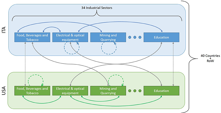
Figure 1. Schematic of the world input-output tables. The WIOT contain data for the domestic production and the export of 34 industrial sectors in 40 countries, plus a model for the remaining countries (named Rest of the World—RoW). In this Figure, for simplicity, we show two countries Italy (ITA) and USA with some industrial sectors. Gray lines represent import/export flows, colored lines trades internal to a country, dashed lines self-consumption of a sector, and dotted lines trades between the same industrial sector of two different countries.

Internal and export flows show high variability in terms of volume from country to country. A better parameter to estimate the importance of an industrial sector is the share with respect to the country's overall internal production or export. Hence, for each industrial sector of each country, we define an internal share i_sc and an export share e_sc. The former reflects the importance of that sector relative to the country's internal economy while the latter reflects its importance relative to the country's export. Shares are defined as:

where s′ runs over all the 34 industrial sectors.

The main goal of this work is to measure the similarity and the similarity's statistical significance of domestic and export shares sector-wise and country-wise.

2.2. Sector-Wise Analysis

Let us first consider the sector-wise similarity. We thus want to measure sector-by-sector whether domestic shares mirror export shares for the available countries. Being n the number of countries, we define ${\text{d}}_s=\left\{i_{s{c}^1},i_{s{c}^2},...,i_{s{c}^n}\right\}$ the vector specifying the domestic shares of a product across countries and ${\text{e}\text{x}}_s=\left\{e_{s{c}^1},e_{s{c}^2},...,e_{s{c}^n}\right\}$ the vector of the corresponding export shares. We measure the per sector similarity as the sample Pearson correlation of the vectors d_s and ex_s. The limited number of countries (n = 41) and the consequent limited statistics make a robust statistical validation of the measured correlation essential. We then require strategies in order to exclude that the sample correlation we observe is associated with a vanishing correlation for the underlying population, i.e., ρ = 0: where ρ is the population correlation coefficient. We will denote population correlation with Greek letters while sample correlation by Roman letters. The statistical validation of correlation can be achieved using different strategies; we will perform the most common ones and discuss the similarities of results witnessing the robustness of our basket of analyses. In detail:

• Mitigation of outliers' role (analysis I): to study the typical range of variability of the observed sample correlation coefficient between the domestic and the export shares, we develop a bootstrapping procedure. Unfortunately domestic and export shares occasionally show a broad distribution and therefore we may occasionally fall into an outlier-type regime for some sectors. We then devise a procedure to mitigate the effect of outliers to test the robustness of our findings. The procedure combines a modified bootstrap with a permutation test and it is easily described by means of a concrete example. In Figure 2A, we show the scatter plot of the internal shares and export shares, i.e., d_s and ex_s, for two sectors (namely Electrical and Optical Equipment and Inland Transport). Each point in the graph represents a country. The sample correlation coefficient of these data is calculated through a modified bootstrapping to mitigate the possible effects of outliers. We essentially re-sample many subsets of the original pairs (further details are provided in Methods section). This permits to evaluate the typical range of variability of the correlation coefficients as shown by the histogram in Figure 2B. We define the sample correlation coefficient r for this sector as the average of the data in this histogram (pointed out by the vertical dotted black line in the same figure panel). To assess the significance of the obtained r we develop a p-value analysis: for each data subset extracted during the bootstrap we calculate the p-value as the results of a permutation test (see section Methods for further details). We then construct the cumulative distribution function of the obtained p-values, shown in Figure 2C. A significant correlation is usually attested by a low p-value. This translates in a p-values' cumulative distribution approaching 1 for small p-values. In the examples shown in Figure 2 this is the case for the “Electrical and Optical equipment” industrial sector, while it is not the case for “Inland transport.” We set a threshold T = 0.15 to define a sector correlated or not. If the 70th percentile of the p-values distribution is below T then the sector is said to be correlated otherwise it is not. We marked in panel (c) of the same figure the 70th percentile of the data by a dotted black line and the 0.15 threshold by a dashed red line. We see that for the “Electrical and Optical Equipment” sector the 70th percentile of the data is well below the threshold. This means that the internal share d_s and ex_s of this sector are significantly correlated as measured by our definition of statistical significance. Vice versa for “Inland Transport” the 70th percentile of the data is greater than the threshold meaning a lack of a significant correlation.

• Confidence level assessment via simple bootstrapping (analysis II): to visualize the comparison of the sample correlation confidence level, we also performed a standard bootstapping procedure. We perform a sampling with replacement of n pairs from the original pairs defining our sample and, by repeating several times this procedure, we can estimate the distribution characterizing the sample correlation variability.

• Permutation test (analysis III): to compare the sample's correlation information with a null model we perform a permutation test shuffling d_s (or alternatively ex_s) and subsequently measuring the correlation and repeat several times this procedure in order to build the ensemble corresponding to the null case we want to exclude, i.e., the zero correlation scenario. A slightly different way to estimate the sample correlation distribution is to generate n pairs of uncorrelated (normal) random numbers, measure the correlation and repeat the procedure several times. Both procedures allow to define a p-value for the observed sample correlation under the null hypothesis ρ = 0. In this work we will provide both approaches.

• Fisher transformation (analysis III): a different approach consists in characterizing the statistics of the sample correlation provided the value of the population correlation ρ. Unfortunately this statistics is Gaussian only for zero population correlation preventing the use of t-statistics. However, it has been shown that the statistics of a non-linear transformation of the sample correlation r- the Fisher transformation - is approximately Gaussian. In detail the variable F(r) = 1/2[ln((1 + r)/(1 − r))] approximately follows a Gaussian distribution with mean μ_ρ = F(ρ) and variance ${\sigma }_{\rho }^2=1/(n-3)$ where n is the sample size. It follows that the p-value of the sample correlation r under the null hypothesis ρ = 0 can be retrieved from the z-score $z=(F(r)-{\mu }_{\rho })/{\sigma }_{\rho }=F(r)\sqrt{n-3}$.

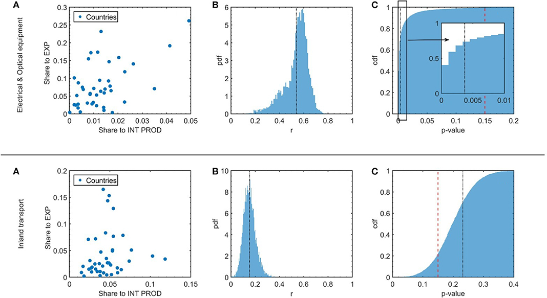
Figure 2. Correlation assessment. The first row refers to a sector where output shares toward export and toward internal production are highly correlated; the second row, a sector for which the correlation is weak. For each row, we present: (A) the scatter plot of countries' export share vs. countries' internal-production share; (B) the histogram of the bootstrap replications and (C) the cumulative distribution of the p-values relative to the bootstrap replications in (B), obtained through data reshuffling. The red dashed line represents the threshold we use to define correlations.

2.2.1. Sector Analysis I: Outlier Mitigation

In Figure 3, we present the 70th percentile p-value for all the sectors in the years from 1996 to 2011. They are sorted by the p-value in 2011 and the sector names belonging to the services [51] are in bold text. We identify sectors for which the correlation is validated and sectors for which is not. Visually, we see that the service sectors are mostly at the bottom of the figure and they present a large p-value for most of the years analyzed. This reflects the fact that for those factor there is not a statistically significant correlation between the domestic production and the export. The three analyses underline the same trend in terms of validated and non-validated sectors (see Supplementary Information for detailed graphs).

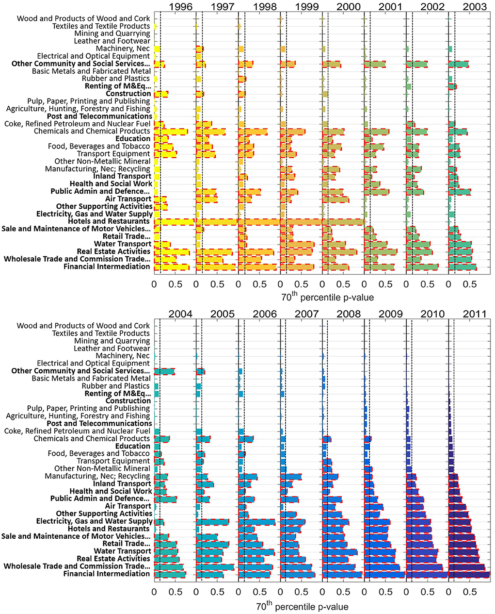
Figure 3. Industrial sectors' correlation. Bars represent the p-values' 70th percentile. Data are sorted according to 2011 p-values. A clear clustering is present: service-related sectors (in bold) do not present a statistically validated correlation between the domestic output and the export. Sectors belonging to the manufacturing and raw material industries have a low p-value hence a robust correlation. Vertical black dashed lines represent the threshold (T = 0.15) to define correlated sectors. with red edges have a p-value larger than T. Sectors are sorted according to their 2011 p-value.

In general, a clear clustering is present between two categories of sectors:

• Sectors showing a statistically significant correlation: “Wood and Products of Wood and Cork,” “Agriculture, Hunting, Forestry and Fishing,” “Textiles and Textile Products,” “Mining and Quarrying,” “Leather, Leather and Footwear,” “Pulp, Paper, Printing and Publishing,” “Basic Metals and Fabricated Metal,” “Electrical and Optical Equipment,” “Post and Telecommunication.” We note that, with the only exception of “Post and Telecommunication,” all these sectors belong to the manufacturing and raw materials industries.

• Sectors not showing a significant correlation: “Inland Transport,” “Health and Social Work,” “Public Admin and Defense; Compulsory Social Security,” “Air Transport,” “Other Supporting and Auxiliary Transport Activities; Activities of Travel Agencies,” “Electricity, Gas, and Water Supply,” “Hotels and Restaurants,” “Sale, Maintenance and Repair of Motor Vehicles and Motorcycles; Retail Sale of Fuel,” “Retail Trade, Except of Motor Vehicles and Motorcycles; Repair of Household Goods,” “Water Transport,” “Real Estate Activities,” “Wholesale Trade and Commission Trade, Except of Motor Vehicles and Motorcycles,” “Financial Intermediation.” Those sectors, all belonging to services, present a p-value higher than T for most of the years considered in this analysis.

The general ordering of the sectors in terms of the significance of the measured correlation and in particular the different behavior for manufacturing and service sectors is robust across all the years available and not specific of a limited time period. However, few exceptions and trends can be spotted. A more explicit visualization of the evolution of significance in time is provided in Figure S3 where we show the time evolution of the 70th percentile p-value from 1996 to 2011 for each sector. We identify a temporal trend for some industrial sectors. In particular “Food, Beverages and Tobacco,” “Coke, Refined Petroleum and Nuclear Fuel,” “Chemicals and Chemical Products,” “Machinery, Nec,” and “Transport Equipment” show an increase in the correlation significance between internal share and export share in the period considered. On the contrary, the industrial sectors “Other Non-Metallic Mineral,” “Manufacturing, Nec; Recycling,” “Electricity, Gas and Water Supply,” “Sale, Maintenance and Repair of Motor Vehicles and Motorcycles; Retail Sale of Fuel” and “Retail Trade, Except of Motor Vehicles and Motorcycles; Repair of Household Goods” show a clear worsening of the correlation significance between the two quantities with time. Several factors may share a role in shaping the similarity between internal and export production. As a general consideration, an increasing correlation may be a signature for an increasing globalization and a reduction of trade barriers. However, underpinning the origin of the forces underlying these trends is beyond the scope of this work.

The general ordering of sectors by statistical significance induced by the different tests proposed exhibits minor differences. However, two common features are shared by all analyses:

1. Statistical significance of domestic and export shares similarity tends to increase in time. We argue this may due to increasing trade liberalization and openness together with more integrated global value chain;

2. Two groups of sectors emerge in a consistent way in the period under investigation. One group, composed of sectors related to the manufacturing and raw material industries, present a significant correlation between the domestic output and the export. This correlation is instead not significant for another group of sectors composed of service-related sectors.

2.2.2. Sector Analysis II: Simple Bootstrap Results

The correlation coefficient between domestic and export shares of the statistically validated sectors are typically observed in the range 0.2−0.9 as shown in Figure S2 and tend to increase over time. Interestingly negative coefficients are usually never statistically validated.

2.2.3. Sector Analysis III: Permutation Test and Fisher Transformation Results

In Figure S1, we show two Yes-No grids summarizing the statistical validation of the sample correlations we measure for the 34 sectors available, respectively, for the two permutation tests we propose and the Fisher transformation. Sectors are ordered according to decreasing p-value in 2011. Ordering is similar but few differences apply. A green plain dot corresponds to p ≤ 0.05, empty red squares to non-validated sectors. As a first result, both strategies provide essentially the same results and, more interestingly, we observe that non-validated sectors tend to be service-related sectors. Detailed p-value tables are provided in the Supplementary Information.

2.3. Country-Wise Analysis

So far we have seen that industrial sectors can be approximately classified into two groups on the basis of the statistical significance of the correlation between domestic and export shares. On average, export is a good proxy for domestic production for manufacturing sectors. Let us now consider the second cross-section analysis we are interested in: the country-wise analysis. Specifically, we want to investigate whether there exist country-specific patterns for the relationship between export and domestic production. In this section we will deal directly with flows (I_sc and E_sc) instead of shares since we do not have scaling issues between flows from different countries, as in the previous section.

We estimate the statistical robustness of per country correlations with the same methods we used for sector-wise analyses, namely permutation tests, Fisher transformation, bootstrap and the test with mitigation of outliers' effects. Referring to Figure 2 again, the general framework is similar: we still consider scatter plots as in panel (a) but now they have log(I_sc) and log(E_sc) on the horizontal and vertical axis, respectively, i.e., the internal flows of sectors and the export flow of the same sectors for a specified country.

In this section, we will run all the statistical tests proposed with two setups: excluding and keeping those sectors which are discarded by the outlier mitigated test discussed in the previous section. Discarded sectors can be retrieved year-by-year from Figure 3 (they are identified by a red dashed edge).

2.3.1. Country Analysis I: Outlier Mitigation

We define as $p_{c,yr}^{all}$ and p_{c, yr} the 70th percentile p-value calculated with all sectors and with only the validated sectors, respectively. We present the results of this analysis in Figure 4 for the years ranging from 1996 to 2011. Solid black lines represent $p_{c,yr}^{all}$ while colored bars represent p_{c, yr}. The color of the bar is:

• Light green if $p_{c,yr}^{all}>T$ and p_{c, yr} < T, i.e., the correlation is statistically significant only excluding the discarded sectors in the sector-wise analysis;

• Dark green if $p_{c,yr}^{all}<T$ and p_{c, yr} < T, i.e., in both cases the correlation is statistically significant. However, we note that $p_{c,yr}^{all}$ tends to be always larger than p_{c, yr}, therefore the case excluding services tends to be more significant from a statistical point of view;

• Dark red if $p_{c,yr}^{all}>T$ and p_{c, yr} > T, i.e., the correlation is not statistically significant in both cases;

• And light red if $p_{c,yr}^{all}<T$ and p_{c, yr} > T, i.e., excluding the discarded sectors decrease the statistical significance of the correlation between internal flows and export flows.

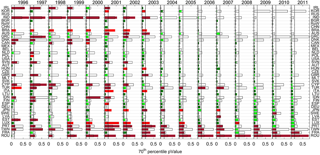
Figure 4. Internal output and export correlation on countries. Bars represent the 70th percentile p-values calculated on countries. These are calculated considering all the sectors (solid black lines) and excluding non-correlated industrial sectors (colored bars). We refer to the text for bar color scheme.

A visual inspection of Figure 4—countries are ordered with respect to p_{c, yr} in 2011—reveals that the vast majority of countries show a notable increase in the significance and of the correlation itself after the removal of the non-validated sectors in the sector-wise analysis. This visually corresponds to the fact that empty bars are larger than colored ones for almost all countries. For instance, in year 2011 only 24 countries out of 41 have validated correlation coefficients including all sectors, after removing not-validated sectors, only 3 countries (i.e., France, Romania, and Taiwan) are not validated as statistically correlated in the country-wise analysis.

The second main observation revealed by the visual inspection of Figure 4 is the presence of a well-defined temporal trend which sees the growth of the number of validated correlation coefficients between export and internal production during the considered period. We have already identified this trend in the sectors' analysis (Figure 3) considering that the 70th percentile of the p-value is overall lower in the last years compared to the previous. However, in this perspective the country-wise analysis is a more suitable playground to look at structural changes of trades (Figure 4). We observe that there is a clear increase of green bars over time. Light red bars completely disappear after 2008 and as mentioned in the last year available the correlation is validated for 37 countries out of 40.

This implies that country's specific patterns are disappearing and export is a good probe for internal output for the majority of the countries we can test. A tentative explanation of this behavior can be rooted in the evolution and the rise of world trades due to the globalization process and to the reduction of trade barriers in the period studied. In particular starting from 2008 a very high correlation between export and internal production is present for the vast majority of countries taken under exam.

Interestingly, most of the countries for which the correlation fails to be validated can be easily interpreted. Starting with persistent red light bars which are, in the perspective of the previous section, the most surprising cases, we find for instance Luxembourg which is indeed an economy traditionally dominated by services. We also find Italy but, as argued in Di Clemente et al. [13], Italy's economic system has evolutionary features which are peculiar and may affect the internal output. We do not have instead obvious interpretation of Brazil's behavior in the late nineties and Japan's one in the early 00s. Turkey and India trends toward an increasing correlation underpin their rising economic trajectories which is leading both countries to be pivotal nodes in the trade network.

A persistent anomaly with respect to the observed positive trend is represented by Romania where not only the correlation is lacking for all the years considered but also removing the non-correlated sectors worsens the situation. Regarding France and Taiwan, in some years the correlation is missing but still we find an improvement by removing the selected sectors. France's trade network appear to have specific features since also in [18] some anomalies have been detected.

2.3.2. Country Analysis II: Simple Bootstrap Results

The correlation coefficient between domestic ad export shares of the statistically validated countries are typically observed in the range 0.0−0.8 as shown in Figure S5. The red bands correspond to the case with all sectors while blue bands to the case with validated sectors only.

2.3.3. Country Analysis III: Permutation Test and Fisher Transformation Results

In Figure S4, we show two Yes-No grids summarizing the statistical validation of the sample correlations we measure for the 41 countries available, respectively, for the two permutation tests we propose and the Fisher transformation. In all cases we provide the results keeping and discarding non-validated sectors. Countries are ordered according to decreasing p-value in 2011. As for sectors, a green plain dot corresponds to p ≤ 0.05, empty red squares to non-validated countries. As a first result, both strategies provide essentially the same results, a country validated by the permutation tests is also validated by Fisher test. However, major differences apply when we discard non-validated sectors (the small symbols aside larger ones represent the results in this latter case). Discarding non-validated sectors we observe that an increasing trend of validated countries occur and the majority of countries is validated in 2011. Detailed p-value tables are provided in the Supplementary Information.

3. Discussion

World Input-Output tables allow us to investigate, at an aggregate level, the relationship between the two parts of the economic output of a country: export and domestic production. The former part can be leveraged as a proxy for cross country production differences in order to assess country competitiveness. So a natural question arises, namely to what extent the fully competition-driven part of a country output, the export, is mirroring the domestic production network features and whether significant differences apply between the two parts. Input-Output tables allow making a substantial direct comparison as they provide sector output flows broken down into domestic and foreign contributions. The relation holds country-wise, even if few exceptions exist, as in the case of Romania.

The main finding is instead the existence of a sector-wise pattern of validity of statistical equivalence between domestic and export-destined production. While export mirrors domestic production structure for manufacturing sectors, the relationship fades away for services sectors. This implies that services export cannot be interpreted as in the case of manufacturing or physical goods: on the contrary, services are economic products characterized by an elusive and subtle nature, which shares features of both products and endowments/capabilities.

We point out, however, that this result does not necessarily question a straightforward extension of country competitiveness measures to services [47, 48], by simply making use of data on international trade. Indeed, services are very different in nature from manufacturing, and are far less tradable; this shows up in the results of the present work. However, the economic complexity framework tries to track the hidden capabilities of countries, and these could emerge in a clearer way by looking to exports than to internal production, given the fact that the international competition plays a major role in the former.

In any case, this analysis is setting constraints and caveats on the general meaning of services export on a competitive basis. Services are economic activities for which geographical localization is often hard. For some of these activities the concept of localization is likely ill-defined, as in the case, for instance, of strategic consulting firms whose teams and project operate worldwide.

The results also provide a perspective to reconcile manufacturing and services sectors in order to join the two dimensions. Starting from those few countries for which export and domestic services are correlated one should first understand at an aggregate level how these two parts are mutually linked. Then, by segmenting countries on the basis of the domestic services diversity similarity, we can try to extend the mapping provided for those countries where the relationship holds to the countries belonging to the same cluster but for which there is a missing correlation between domestic services and services export. Provided in this way a scheme to estimate how to reconcile export and domestic services diversity and a re-scaling profile for each country, this mapping can be eventually extended at a disaggregate level.

4. Methods

4.1. Datasets

We used data extracted from World Input Output Tables (WIOT) [45, 46]; they consist in 17 different tables, one for each year from 1995 to 2011. The structure of the table is a matrix that lists economic sectors associated to countries, in the same sequence, both vertically and horizontally. Values on the column represent inputs for the industrial sector and the country at the beginning of the column, expressed in monetary value; while the values on the row represent outputs from the sector and the country at the beginning of the row. Thus, any sector can be analyzed in terms of the direction and amount of its inputs and outputs. We used only the information relative to the fluxes exchanged between industrial sectors of all the countries considered in the database, which covers 27 European countries and 13 other major countries in the world. The 40 countries considered cover more than 85% of world gross domestic product (GDP) in 2008. A model for the Rest of the World (RoW), which accounts for the remaining 15% of world GDP, is used to predict the remaining trades. Each table contains fluxes in current US dollars between 35 industrial sectors. Fluxes both inside the same economy and toward foreign economies are reported. We use only data for 34 sectors since ‘Private Households with Employed Persons’ has often null input or output. WIOT also provides data for the final demand, government expenditures, depreciation of capital, taxes, etc. However, we do not use these data for a two-fold reason. On one hand, we are interested in the inter-industrial trades. On the other hand, by performing an analysis of competitiveness for countries as in Tacchella et al. [19] using export flows derived from WIOD dataset, we obverse that correlation with the results of the same analysis run on bilateral trade flows is higher when we remove final consumption, especially when services are included in the analysis. This again points in the direction of a non-trivial relationship between domestically-consumed and exported services.

4.2. Sector Names

Throughout the paper we used shortened versions of the WIOT sectors' names. In Supplementary Information, we provide the mapping of those shortened names with WIOD ones.

4.3. Correlation Significance Assessment for Sectors: Outlier Mitigation (Analysis I)

Our aim is to study the correlation between the internal production of a country and its export. We define these quantities correlated if the p-value of the correlation coefficients' distribution is lower then T = 0.15. We can in this way exclude having an accidental correlation between internal production and export. As a first step, we need a method that allows eliminating outliers from our data set in a systematic way, so that they do not influence the value of the correlation coefficient. For this reason, we perform a bootstrap using only 80% of data, randomly drawn, and we calculate the correlation coefficient only on these data. We repeat this operation 2, 500 times, in this way it is possible to build an empirical distribution measuring the typical range of the correlation coefficients (as shown in Figure 3). In order to assess the statistical robustness of the correlation coefficients, for each bootstrapped subsets we calculated the p-value (this means we now have 2,500 p-values). Each p-value is estimated by reshuffling bootstrapped subset data 5,000 times and by calculating the percentile corresponding to the correlation coefficient of the bootstrapped subset with respect to the correlation distribution obtained from this random ensemble. If the 70th percentile of the p-values distribution is below T then the sector is said to be correlated, otherwise it is not.

It is worth noticing that this approach is robust against noise thanks to the bootstrapping and the calculation of p-values on the bootstrapped data. This is a necessity when dealing with this kind of data, which naturally present outliers and a component of noise.

4.4. Correlation Significance Assessment for Countries: Outlier Mitigation (Analysis I)

When we study the correlation between internal production and export relative to each country we deal directly with fluxes instead of shares. Indeed, in this case, we do not mix up data from different countries. Eventually the values that we take for the comparison are the log of the internal flux log(I_sc) and the log of the export flux log(E_sc).

The procedure we adopted to establish the correlation is exactly the same used for products. We obtain the p-value relative to the 70th percentile of the distribution if its lower than T for that country export is a good probe of internal production otherwise it is not.

Data Availability Statement

WIOD dataset is publicly available and can be downloaded from the website (www.wiod.org/home).

Author Contributions

MC, AT, and AZ developed the logic for these ideas and designed the analysis. MC, FS, and VC performed the numerical simulations and experiments. All five authors were involved in writing the paper. All authors developed the formal analysis and explored the data.

Funding

CNR Progetto di Interesse CRISISLAB covered the salaries of MC, AT, and AZ. The funders had no role in study design, data collection and analysis, decision to publish, or preparation of the manuscript.

Conflict of Interest

The authors declare that the research was conducted in the absence of any commercial or financial relationships that could be construed as a potential conflict of interest.

Acknowledgments

MC, AT, and AZ thank CNR Progetto di Interesse CRISIS LAB for supporting their research activity.

Supplementary Material

The Supplementary Material for this article can be found online at: https://www.frontiersin.org/articles/10.3389/fphy.2020.00180/full#supplementary-material

References

1. Bouchaud J-P. Economics needs a scientific revolution. Nature. (2008) 455:1181. doi: 10.1038/4551181a
3. Hommes CH. Financial markets as nonlinear adaptive evolutionary systems. Quant Fin. (2001) 1:149–67. doi: 10.1080/713665542
4. Acemoglu D, Carvalho VM, Ozdaglar A, Tahbaz-Salehi A. The network origins of aggregate fluctuations. Econometrica. (2012) 80:1977–2016. doi: 10.3982/ECTA9623
5. Squartini T, Garlaschelli D. Analytical maximum-likelihood method to detect patterns in real networks. N J Phys. (2011) 13:083001. doi: 10.1088/1367-2630/13/8/083001
6. Garlaschelli D, Loffredo MI. Structure and evolution of the world trade network. Phys A Stat Mech Appl. (2005) 355:138–44. doi: 10.1016/j.physa.2005.02.075
7. Fagiolo G, Reyes J, Schiavo S. World-trade web: Topological properties, dynamics, and evolution. Phys Rev E. (2009) 79:036115. doi: 10.1103/PhysRevE.79.036115
8. Cimini G, Squartini T, Gabrielli A, Garlaschelli D. Estimating topological properties of weighted networks from limited information. Phys Rev E. (2015) 92:040802. doi: 10.1103/PhysRevE.92.040802
9. Battiston S, Puliga M, Kaushik R, Tasca P, Caldarelli G. Debtrank: Too central to fail? Financial networks, the fed and systemic risk. Sci Rep. (2012) 2:541. doi: 10.1038/srep00541
10. Poce G, Cimini G, Gabrielli A, Zaccaria A, Baldacci G, Polito M, et al. What do central counterparty default funds really cover? A network-based stress test answer. J Netw Theory Fin. (2018) 4:43–57. doi: 10.21314/JNTF.2018.047
11. Farmer JD, Lafond F. How predictable is technological progress? Res Policy. (2016) 45:647–65. doi: 10.1016/j.respol.2015.11.001
12. Pugliese E, Cimini G, Patelli A, Zaccaria A, Pietronero L, Gabrielli A. Unfolding the innovation system for the development of countries: coevolution of science, technology and production. Sci Rep. (2019) 9:16440. doi: 10.1038/s41598-019-52767-5
13. Di Clemente R, Chiarotti GL, Cristelli M, Tacchella A, Pietronero L. Diversification versus specialization in complex ecosystems. PLoS ONE. (2014) 9:e112525. doi: 10.1371/journal.pone.0112525
14. Pugliese E, Napolitano L, Zaccaria A, Pietronero L. Coherent diversification in corporate technological portfolios. PLoS ONE. (2019) 14:e223403. doi: 10.1371/journal.pone.0223403
15. Teece DJ, Rumelt R, Dosi G, Winter S. Understanding corporate coherence: theory and evidence. J Econ Behav Organ. (1994) 23:1–30. doi: 10.1016/0167-2681(94)90094-9
16. Hausmann R, Hwang J, Rodrik D. What you export matters. J Econ Growth. (2007) 12:1–25. doi: 10.1007/s10887-006-9009-4
17. Hidalgo CA, Klinger B, Barabási A-L, Hausmann R. The product space conditions the development of nations. Science. (2007) 317:482–7. doi: 10.1126/science.1144581
18. Hidalgo C. A, Hausmann R. The building blocks of economic complexity. Proc Natl Acad Sci USA. (2009) 106:10570–5. doi: 10.1073/pnas.0900943106
19. Tacchella A, Cristelli M, Caldarelli G, Gabrielli A, Pietronero L. A new metrics for countries' fitness and products' complexity. Sci Rep. (2012) 2:723. doi: 10.1038/srep00723
20. Zaccaria A, Cristelli M, Tacchella A, Pietronero L. How the taxonomy of products drives the economic development of countries. PLoS ONE. (2014) 9:e113770. doi: 10.1371/journal.pone.0113770
21. Cristelli M, Tacchella A, Pietronero L. The heterogeneous dynamics of economic complexity. PLoS ONE. (2015) 10:e0117174. doi: 10.1371/journal.pone.0117174
22. Pugliese E, Zaccaria A, Pietronero L. On the convergence of the fitness-complexity algorithm. Eur Phys J Spcl Top. (2016) 225:1893–911. doi: 10.1140/epjst/e2015-50118-1
23. Zaccaria A, Cristelli M, Kupers R, Tacchella A, Pietronero L. A case study for a new metrics for economic complexity: the Netherlands. J Econ Interact Coord. (2016) 11:151–69. doi: 10.1007/s11403-015-0145-9
24. Pugliese E, Chiarotti GL, Zaccaria A, Pietronero L. Complex economies have a lateral escape from the poverty trap. PLoS One. (2017) 12:e0168540. doi: 10.1371/journal.pone.0168540
25. Cimini G, Gabrielli A, Labini FS. The scientific competitiveness of nations. PLoS ONE. (2014) 9:e113470. doi: 10.1371/journal.pone.0113470
26. Smith A, Nicholson JS. An Inquiry Into the Nature and Causes of the Wealth of Nations. London: T. Nelson and Sons (1887).
29. Aghion P, Howitt P. A model of growth through creative destruction. Econometrica. (1992) 60:323–51. doi: 10.2307/2951599
30. Romer PM. Endogenous technological change. J Polit Econ. (1990) 98:S71–S102. doi: 10.1086/261725
32. Leontief W. Domestic production and foreign trade; the American capital position re-examined. Proc. Am. Philos. Soc. (1953) 97:332–49.
33. Leontief W. Factor proportions and the structure of American trade: further theoretical and empirical analysis. Rev. Econ Stat. (1956) 38:386–407. doi: 10.2307/1926500
34. Solow RM. A contribution to the theory of economic growth. Q J Econ. (1956) 70:65–94. doi: 10.2307/1884513
35. Barro RJ. Economic Growth in a Cross Section of Countries. Technical Report. National Bureau of Economic Research (1989).
36. Sbardella A, Pugliese E, Zaccaria A, Scaramozzino P. The role of complex analysis in modelling economic growth. Entropy. (2018) 20:883. doi: 10.3390/e20110883
37. Ashraf Q, Galor O. The ‘out of Africa’ hypothesis, human genetic diversity, and comparative economic development. Am Econ Rev. (2013) 103:1–46. doi: 10.1257/aer.103.1.1
38. D'Alpoim Guedes J, Bestor TC, Carrasco D, Flad R, Fosse E, Herzfeld M, et al. Is poverty in our genes? A critique of Ashraf and Galor, “The ‘Out of Africa’ Hypothesis, Human Genetic Diversity, and Comparative Economic Development”. American Economic Review (Forthcoming). Curr Anthropol. (2013) 54.1:71–9.
39. Lall S, Weiss J, Zhang J. The ‘sophistication’ of exports: a new trade measure. World Dev. (2006) 34:222–37. doi: 10.1016/j.worlddev.2005.09.002
40. Cristelli M, Gabrielli A, Tacchella A, Caldarelli G, Pietronero L. Measuring the intangibles: A metrics for the economic complexity of countries and products. PLoS ONE. (2013) 8:e70726. doi: 10.1371/journal.pone.0070726
41. Tacchella A, Cristelli M, Caldarelli G, Gabrielli A, Pietronero L. Economic complexity: conceptual grounding of a new metrics for global competitiveness. J Econ Dyn Control. (2013) 37:1683–91. doi: 10.1016/j.jedc.2013.04.006
42. Annunziata MA, Petri A, Pontuale G, Zaccaria A. How log-normal is your country? An analysis of the statistical distribution of the exported volumes of products. Eur Phys J Spcl Top. (2016) 225:1985–95. doi: 10.1140/epjst/e2015-50320-7
43. Feenstra RC, Lipsey RE, Deng H, Ma A. C, Mo H. World Trade Flows: 1962-2000. Technical Report. National Bureau of Economic Research (2005). doi: 10.3386/w11040
44. Gaulier G, Zignago S. Baci: international trade database at the product-level (the 1994–2007 version). CEPII Working Paper 2010–23. (Paris) (2010). doi: 10.2139/ssrn.1994500
45. Dietzenbacher E, Los B, Stehrer R, Timmer M, De Vries G. The construction of world input-output tables in the wiod project. Econ Syst Res. (2013) 25:71–98. doi: 10.1080/09535314.2012.761180
46. Timmer MP, Dietzenbacher E, Los B, Stehrer R, Vries GJ. An illustrated user guide to the world input-output database: the case of global automotive production. Rev Int Econ. (2015) 23:575–605. doi: 10.1111/roie.12178
47. Stojkoski V, Utkovski Z, Kocarev L. The impact of services on economic complexity: service sophistication as route for economic growth. PLoS ONE. (2016) 11:161633. doi: 10.1371/journal.pone.0161633
48. Zaccaria A, Mishra S, Cader M. Z, Pietronero L. Integrating services in the economic fitness approach. World Bank Policy Res Work Pap. (2018). doi: 10.1596/1813-9450-8485
50. Cerina F, Zhu Z, Chessa A, Riccaboni M. World input-output network. PLoS ONE. (2015) 10:e0134025. doi: 10.1371/journal.pone.0134025
51. Timmer M, Erumban AA, Gouma R, Los B, Temurshoev U, de Vries GJ, et al. The World Input-Output Database (WIOD): Contents, Sources and Methods. Institue for International and Development Economics (2012). Available online at: https://ideas.repec.org/p/lnz/wpaper/20120401.html
Keywords: economic complexity, services, industrial production, WIOD, economic fitness
Citation: Saltarelli F, Cimini V, Tacchella A, Zaccaria A and Cristelli M (2020) Is Export a Probe for Domestic Production? Front. Phys. 8:180. doi: 10.3389/fphy.2020.00180
Received: 28 January 2020; Accepted: 27 April 2020;
Published: 26 June 2020.
Edited by:
Damien Challet, Université Paris-Saclay, FranceReviewed by:
Matúš Medo, University of Electronic Science and Technology of China, ChinaAlessandro Pluchino, University of Catania, Italy
Copyright © 2020 Saltarelli, Cimini, Tacchella, Zaccaria and Cristelli. This is an open-access article distributed under the terms of the Creative Commons Attribution License (CC BY). The use, distribution or reproduction in other forums is permitted, provided the original author(s) and the copyright owner(s) are credited and that the original publication in this journal is cited, in accordance with accepted academic practice. No use, distribution or reproduction is permitted which does not comply with these terms.
*Correspondence: Andrea Zaccaria, andrea.zaccaria@cnr.it
†These authors have contributed equally to this work