Responses of a two degrees-of-freedom system with uncertain parameters in the vicinity of resonance 1:1

Abstract

We analyze the dynamics of a nonlinear mechanical system under the influence of an external harmonic force. The system consists of a linear oscillator (primary mass) and attached nonlinear dynamic absorber. It is supposed that the frequency of the external force is close to the natural frequency of the main mass. Assuming that the parameters of the system are uncertain, the stability conditions of the stationary regimes of the averaged equations are obtained analytically; these regimes correspond to the quasi-periodic motions of the original input system. An analytical approach to the problem of selecting the parameters of a dynamic absorber is proposed in order to reduce the amplitude of oscillations of the main system. The results obtained are compared with the results of the numerical integration of the equations of the motion with different initial conditions and parameter values.

1 Introduction

In recent decades, a number of researchers have made significant efforts to solve the problem of dissipating the excessive vibration energy of mechanical systems. Vibration isolation and control is one of the most important areas of engineering research, which aims to prevent the transmission of unwanted vibrations of a basic structure to neighboring systems or to eliminate or reduce excessive vibration in the main system in order to avoid possible damage. Elimination, reduction or isolation of oscillations is the main problem of various industrial and technical practices. The use of a device to reduce the resonant vibrations firstly has been patented by Frahm [1], and later have been presented in more formalized and detailed form by Ormondroyd [2], Den Hartog [2, 3] and Brock [4]. Such vibration absorber represents a dashpot consisting of a mass connected with the main system by spring with viscous damping. Through the proper tuning of the absorber (stiffness of the spring and damping coefficient), it is possible to minimize the frequency response in the vicinity of the target resonant frequency. Such a device is addressed in the literature as dynamic vibration absorber (DVA or LDVA) or tuned mass damper (TMD).

As many researchers have noted later on, linear vibration absorbers are effective only in a very narrow band of excitation frequencies, in other words, their frequency robustness is low. To overcome this obstacle and increase the frequency bandwidth, different nonlinear spring characteristics have been introduced. Roberson [5] proposes a dynamic vibration absorber with a weakly nonlinear spring characteristic, i.e., a linear spring with small cubic nonlinearity. It was shown that this nonlinear absorber reduces the vibrations over a larger frequency bandwidth compared to its linear counterpart.

More recently, absorbers with a strongly nonlinear spring characteristic (a spring with cubic nonlinearity) have been investigated. In the work of Gendelman [6], the redistribution of the energy of free oscillations of a system with two degrees of freedom consisting of a coupled linear and nonlinear oscillator was investigated. Vakakis and Gendelman showed [7] that energy transfer between weakly coupled linear and nonlinear oscillators is due to transient resonance capture on a resonant 1:1 manifold. Zhu et al. [8] have studied stability and bifurcations in 2-DOF vibration system with nonlinear damping and nonlinear spring. Gendelman and Staroswetsky [9] have demonstrated that the quasi-periodic response regimes are very typical for a periodically forced linear oscillator with the nonlinear energy sink (NES) attached. Jing and Lang theoretically studied [10] the cubic nonlinear damping in the frequency domain through a dimensionless vibration system model actuated by a harmonic input. A qualitative tuning methodology, which imposes the frequency-energy dependence of the absorber to be identical to that of the nonlinear primary system, was developed by Vigui$\acute{\mathrm {e}}$ and Kerschen [11] to mitigate the impulsive response of an SDOF nonlinear oscillator. Petit et al. [12] have focused on the analysis of energy thresholds in 2-DOF system, below which (thresholds) no efficient vibration reduction is possible. The authors proposed a reformulation of the dynamics of the system, leading to the introduction of a new parameter threshold, and their analysis pointed out the regions in parameter space where efficient vibration reduction can be obtained. A novel NES for energy harvesting has been developed by Kremer and Liu [13]. Its spring possesses a strong nonlinear stiffness with a minimum linear component and low mechanical damping. It has been shown that the system is capable of energy localization as well as broadband vibration absorption and energy harvesting. The article of Yang et al. [14] provided an assessment of the dynamic characteristics of a nonlinear absorber attached to a nonlinear primary oscillator from the point of view of the oscillatory power flow. The power factor and kinetic energy of the nonlinear oscillator were used as performance indices. Various combinations of cubic nonlinearities of damping and stiffness in an oscillator and an absorber were investigated.

In the work of Casalotti and Lacarbonara [15] the method of multiple scales was adopted to investigate the 1:1 internal resonance arising in a two-DOF system composed of a nonlinear oscillator coupled with a nonlinear DVA exhibiting hysteresis. Taleshi et al. [16] investigated the targeted energy transfer from a harmonic-excited nonlinear plate to nonlinear and linear attachments with comparison those both. Cirillo et al. [17] have applied singularity theory for nonlinear resonance of a two-degree-of-freedom mechanical system.

Over the past fifteen years, the works of various authors have been devoted to a topic related to the dynamics of a 2-DOF system with nonlinear coupling [18,19,20,21,22,23,24,25,26,27,28,29,30,31,32]. In papers [33,34,35,36], the emphasis was put on optimizing the absorber design as well as design the DVA with special properties [37,38,39]. Mostly the authors used a combination of an analytical approach and numerical methods. Commonly used analytical methods are: multiple scale method [21, 23], averaging of the motion equations [8, 9, 14, 37] harmonic balance method [28, 40], and some combined techniques [41]. Interesting results with experimental study/validation were obtained in papers [24, 31, 42,43,44].

In the present paper, we investigate the dynamics of a 2-DOF system with a nonlinear elastic characteristic and uncertain parameters. The emphasis is placed on the development of an analytical procedure for determining the parameters of the absorber, contributing to the maximum decrease in the amplitude of oscillations of the main system. Numerical calculations are used to verify the results obtained.

The article is structured as follows. In Sect. 2 the equations of motion of a mechanical system are given, which are then reduced to a form suitable for analysis. The method of averaging [45] is applied to simplify the mathematical model and stationary points are found. In Sect. 3, we analyze the stability of equilibria of averaged equations, which correspond to the periodic motions of the mechanical system under study. The necessary and sufficient conditions for asymptotic stability are obtained on the basis of analysis of the linearized system. The joint effect of the damping coefficient and the nonlinear component of the stiffness of DVA onto appearance of the flutter instability is investigated. Section 4 is devoted to studying the influence of the NDVA parameters on the magnitude of the oscillations of the primary mass in the vicinity of resonant frequencies. An analytical approach is proposed for localizing the values of these parameters (tuning the absorber). Section 5 conducts numerical experiments to verify the results obtained. The results of integration of averaged equations and complete equations of motion are compared. Finally, some concluding remarks are provided.

2 Description of the model

The schematic view of a harmonically excited linear oscillator (primary system or LO) coupled with a nonlinear absorber (secondary system or NDVA) is presented in Fig. 1.

Fig. 1

Mechanical system: nonlinear absorber attached to linear SDOF primary system

The equations of motion of this mechanical system are

$$\begin{aligned}&m_1 \ddot{x}_1 + c_a (\dot{x}_1 - \dot{x}_a ) + k_1 x_1 + k_a ^{\mathrm{lin}} (x_1 - x_a )\nonumber \\&\quad - \,k_a ^{\mathrm{nonlin}} (x_1 - x_a )^3 = F_0 \cos \omega t,\nonumber \\&m_a \ddot{x}_a + c_a (\dot{x}_a - \dot{x}_1 ) + k_a ^{\mathrm{lin}} (x_a - x_1 )\nonumber \\&\quad - \,k_a ^{\mathrm{nonlin}} (x_a - x_1 )^3 = 0 \end{aligned}$$

(1)

where $x_1 (t)$ and $x_a (t)$ are the displacements of the harmonically forced primary system and of the damped absorber with a stiffness whose linear and nonlinear coefficients of rigidity are denoted by $k_a ^{\mathrm{lin}}$ and $k_a ^{\mathrm{nonlin}},$ respectively. After adding the second equation of (2) to the first one and introducing the new variable $x_2 = x_a - x_1$ the motion equations may be rewritten in simplified form

$$\begin{aligned}&(m_1 + m_a ) \ddot{x}_1 + m_a \ddot{x}_2 + k_1 x_1 = F_0 \cos \omega t,\nonumber \\&m_a \ddot{x}_1 + m_a \ddot{x}_2 + c_a \dot{x}_2 + k_a ^{\mathrm{lin}} x_2 - k_a ^{\mathrm{nonlin}} x_2 ^3 = 0. \end{aligned}$$

(2)

The subject of our study is the case when natural frequency of the primary mass $\omega _1 = \sqrt{k_1 / m_1}$ is close to the frequency of the external excitation $\omega .$ Taking into account that mass of the absorber is usually much smaller than main mass, i.e., the ratio $m_a / m_1$ may be assumed as small parameter; therefore the ratio $\tilde{\omega }_1 = \sqrt{k_1 / (m_1 + m_a)}$ is also close to $\omega$. We believe that use of the $\tilde{\omega }_1$ instead of $\omega _1$ is accountable, because the natural frequencies of 2-DOF system are changed slightly, and the magnitude $\omega = \omega _1$ is not the “pure” resonant frequency.

Let us introduce the dimensionless parameters and time by formulas

$$\begin{aligned} \omega _1 & = \sqrt{\frac{k_1}{m_1}}, \ {\tilde{\omega }_1 = \sqrt{\frac{k_1}{m_1 + m_a}},} \ \omega _a = \sqrt{\frac{k_a ^{\mathrm{lin}}}{m_a}}, \nonumber \\ \mu & = \sqrt{\frac{m_a}{m_1}}, \ q = \left( \frac{\omega }{\omega _1}\right) ^2,\nonumber \\ \varepsilon & = q - \frac{1}{1+\mu ^2}, \ \gamma = \frac{\omega _a ^2}{\omega _1 ^2} - \frac{1}{1 + \mu ^2}, \ h = \frac{c_a \omega _1}{\mu ^2 k_1}, \nonumber \\ \widetilde{\varkappa } & = \frac{k_a ^{\mathrm{nonlin}} m_1 ^2 F_0 ^2}{k_1 m_a ^2}, \ \tau = \omega t. \end{aligned}$$

(3)

With the aim to reduce the number of parameters, we introduce also the relative displacements by formulas

$$\begin{aligned} x_1 = F_0 \widetilde{x}_1, \ x_2 = \mu F_0 \widetilde{x}_2, \end{aligned}$$

(4)

and now the motion equations are in the following form

$$\begin{aligned} { M \widetilde{x}'' + D \widetilde{x}' + K \widetilde{x} = \varPhi }(\tau , \widetilde{x}_2). \end{aligned}$$

(5)

Here

$$\begin{aligned} {\varvec{M}} & = q \left( \begin{array}{cc} 1 + \mu ^2 &\mu \\ \mu &1 \\ \end{array} \right) , \ \widetilde{{\varvec{x}}} = \left( \begin{array}{c} \widetilde{x}_1 \\ \widetilde{x}_2 \\ \end{array} \right) , \ {\varvec{D}} = {\hbox {diag}}(0, h \sqrt{q}),\nonumber \\ {\varvec{K}} & = {\hbox {diag}}(1, \frac{1}{1 + \mu ^2} + \gamma ), \ \varvec{\varPhi }= \left( \begin{array}{c} {\cos } \tau \\ \widetilde{\varkappa } x_2 ^3 \\ \end{array} \right) , \end{aligned}$$

(6)

where the prime means the derivative on time $\tau$. For convenience, the symbol “$\thicksim$” over $x_1, x_2$ is subsequently discarded.

With the transformation

$$\begin{aligned} x_j & = u_j \cos \tau + v_j \sin \tau , \ x_{j}' = - u_j \sin \tau \nonumber \\&\quad+ \,v_j \cos \tau \ (j=1, 2) \end{aligned}$$

(7)

the following shape of the motion equations (5) appears

$$\begin{aligned}&\cos \tau [\varvec{M {v'} + (- M + K) u + D v}]\nonumber \\&\quad - \,\sin \tau [\varvec{M {u'} + D u + (M - K) v }] = \varvec{\varPhi },\nonumber \\&\cos \tau (\varvec{{u'} + v}) + \sin \tau (\varvec{{v'} - u)} = - \sin \tau {\varvec{u}} + \cos \tau {\varvec{v}}. \end{aligned}$$

(8)

Further, taking the linear combinations $-\sin \tau \cdot (8.1) + \cos \tau {\varvec{M}} \cdot (8.2)$ and $\cos \tau \cdot (8.1) + \sin \tau {\varvec{M}} \cdot (8.2),$ we have the following equations

$$\begin{aligned}&\varvec{M u}' + \frac{1}{2} [(1 - c_2 ) {\varvec{D}} + s_2 (\varvec{M - K})] {\varvec{u}} \nonumber \\&\quad + \,\frac{1}{2} [-s_2 \varvec{D} + (1 - c_2 ) (\varvec{M - K})] {\varvec{v}} = \varvec{\varPhi }_1 ,\nonumber \\&\varvec{M v}' + \frac{1}{2} [- s_2 {\varvec{D}} + (1 + c_2 ) (\varvec{K - M})] {\varvec{u}}\nonumber \\&\quad + \,\frac{1}{2} [(1 + c_2 ) {\varvec{D}} + s_2 ) (\varvec{K - M})] {\varvec{v}} = \varvec{\varPhi }_2 , \end{aligned}$$

(9)

where the right-hand side expressions are defined by formulas

$$\begin{aligned} \varvec{\varPhi }_1 & = - \frac{1}{8} \mathrm {col} (4 s_2 , \widetilde{\varkappa } [(2 s_2 + s_4 ) u_2 ^3 +3 (1 - c_4 )u_2 ^2 v_2\nonumber \\&\quad+\,3 (2 s_2 -s _4 ) u_2 v_2 ^2 + (3- 4 c_2 +c_4 ) v_2 ^3]),\nonumber \\ \varvec{\varPhi }_2 & = \frac{1}{8} \mathrm {col} (4 (1 + c_2 ), \widetilde{\varkappa }[(3 + 4 c_2 + c_4 ) u_2 ^3\nonumber \\&\quad+\, 3 (2 s_2 + s_4 )u_2 ^2 v_2 + 3 (1 - c _4 ) u_2 v_2 ^2 \nonumber \\&\quad+\, (2 s_2 - s_4 ) v_2 ^3]), \ s_2 = \sin 2\tau , \nonumber \\ c_2 & = \cos 2 \tau , \ s_4 = \sin 4 \tau , \ c_4 = \cos 4 \tau . \end{aligned}$$

(10)

Equation (9) are more cumbersome compared to the original Eq. (1), but they have the advantage that the variables $\varvec{u, v}$ change much more slowly over time $\tau$, in contradistinction to “fast” variables $\varvec{x, x'}$. Accordingly, with numerical integration, the calculation fault due to the accumulation of error (which may result in stuck overflow) is more likely for system (1), and dealing with the system (9) is more secure (an illustrative example is presented below).

Fig. 2

Comparing the numerical integration for systems (5) and (9)

Figure 2a refers to time history for $x_1$ component of system (5) ($\mu = 0.236$, $h = 0.256, \gamma = - 0.04, \varepsilon = - 0.15, \varkappa = 0.08)$. As one can see, it may appear the avalanche-like increasing of amplitude (leads to overflow). Figure b, c are related to time histories for $u_1 , v_1$ components for system (9) (with the same values of parameters and corresponding initial values) exhibiting a normal behavior. Though the discussed issue for numerical integration of system (5) does not often happen, but the system (9) is more robust in this respect.

Let us assume that $\varvec{u, v}$ are the slow functions about the time $\tau$. Applying the method of averaging [45], we get the simplified version of the system (9)

$$\begin{aligned}&\varvec{M u}' + \frac{1}{2} [ \varvec{D u} + \varvec{(M - K) v}] = - \frac{3}{8} \widetilde{\varkappa } \left( \begin{array}{c} 0 \\ v_2 ( u_2 ^2 + v_2 ^2) \\ \end{array} \right) ,\nonumber \\&\varvec{M v}' + \frac{1}{2} [\varvec{(K - M) u + D v}] = \frac{3}{8} \left( \begin{array}{c} 4 \\ \widetilde{\varkappa } u_2 ( u_2 ^2 + v_2 ^2) \\ \end{array} \right) , \end{aligned}$$

(11)

which do not contain the time-dependent terms, as all of them have zero average value over $2 \pi$ time period.

Now we shall find the stationary points of the system (11) which correspond to periodic motions with respect to displacements $x_1, x_2$.¹

For the sake of simplicity it is appropriate to introduce the complex variables ${\varvec{z}} = {\varvec{u}} + i \varvec{v}$. Then Eq. (11) takes the following form

$$\begin{aligned}&\varvec{M z}' + \frac{1}{2} ({\varvec{B}} + i \varvec{D) z} = \frac{1}{2} i \left( \begin{array}{cc} 1 \\ \varkappa z_2 ^2 \bar{z}_2 \\ \end{array} \right) , \nonumber \\&\varvec{M \overline{z}}' + \frac{1}{2} ({\varvec{B}} + i \varvec{D) \bar{z}} = \frac{1}{2} i \left( \begin{array}{c} - 1 \\ \varkappa z_2 \bar{z}_2 ^2 \\ \end{array} \right) . \end{aligned}$$

(12)

Here the following notions are introduced

$$\begin{aligned}&\varvec{K - M \triangleq B} = \left( \begin{array}{cc} b_{11} &b_{12} \\ b_{12} &b_{22} \\ \end{array} \right) , \ b_{11} = - \varepsilon (1 + \mu ^2), \nonumber \\&b_{12} = - \mu q, \ b_{22} = \gamma - \varepsilon , \ \varkappa = \frac{3}{4} \widetilde{\varkappa }. \end{aligned}$$

(13)

Thus, with condition $\varvec{z' = 0}$, we have the following system of nonlinear algebraic equations

$$\begin{aligned} b_{11} z_1 + b_{12} z_2 = 1, \ b_{12} z_1 + (b_{22} - i h) z_2 = \varkappa z_2 ^2 \bar{z}_2, \end{aligned}$$

(14)

and their conjugate counterparts for $\bar{z}_1, \bar{z}_2$.

Depending on the value of $b_{11}$, we have two cases.

• (A) $b_{11} = 0$. According to formulas (13) this case may happen only when $\varepsilon = 0,$ which corresponds to “pure” resonant case for system with “frozen” absorber, i.e., $\omega = \omega _0.$ Then, taking into account that $\ b_{12} = - \mu / (1 + \mu ^2 ) \ne 0,$ immediately from Eq. (14) we get

  $$\begin{aligned} z_{20} = \frac{1}{b_{12}}, \ z_{10} = \frac{1}{b_{12}^2} ( - b_{22} + i h + \frac{\varkappa }{b_{12}^2}). \end{aligned}$$

  (15)

  Thus, the system (13) has the unique constant solution (15).

• (B) $b_{11} \ne 0 \ (\varepsilon \ne 0)$. Let us express $z_1$ from the first equation of (14) and substitute it into the second one. It follows from equations

  $$\begin{aligned}&b_{12} + (\varDelta _B - i h b_{11}) z_2 = b_{11} \varkappa z_2^2 \bar{z}_2, \nonumber \\&b_{12} + (\varDelta _B + i h b_{11}) \bar{z}_2 = b_{11} \varkappa z_2 \bar{z}^2_2, \ \varDelta _B = \mathrm {det} {\varvec{B}}. \end{aligned}$$

  (16)

Subtracting the second Eq. (16) from the first one, we write down the auxiliary equality

$$\begin{aligned}&(\varDelta _B - b_{11} \varkappa z_{20} \bar{z}_{20}) ( z_{20} - \bar{z}_{20})\nonumber \\&\quad - \,i h b_{11} ( z_{20} + \bar{z}_{20}) = 0. \end{aligned}$$

(17)

Also we subtract the second Eq. (16) with multiplier $z_{20}$ from the first equation multiplied by $\bar{z}_{20}$. As a result, we have another auxiliary equality

$$\begin{aligned} b_{12} (z_{20} - \bar{z}_{20}) + 2 i h b_{11} z_{20} \bar{z}_{20} = 0. \end{aligned}$$

(18)

Coming back from complex variables to real ones we get the corresponding system

$$\begin{aligned}&{[}\varDelta _B - b_{11} \varkappa (u_{20}^2 + v_{20}^2 )] v_{20} - h b_{11} u_{20} = 0, \nonumber \\&b_{12} v_{20} + h b_{11} (u_{20}^2 + v_{20}^2 ) = 0, \end{aligned}$$

(19)

which is equivalent² to the system (14). Expressing the sum $u_{20}^2 + v_{20}^2$ from the second equation and substituting it in the first one we can express the variable $u_{20}$ in terms of $v_{20}$:

$$\begin{aligned} u_{20} = \frac{1}{h^2 b_{11}} v_{20} (h \varDelta _B + b_{12} \varkappa v_{20}), \end{aligned}$$

(20)

which leads to cubic equation

$$\begin{aligned} P_1 (v_{20}) & = b_{11}^2 \varkappa ^2 v_{20}^3 + 2 b_{11} h \varkappa \varDelta _B v_{20}^2 \nonumber \\&\quad+\, h^2 v_{20} (h^2 b_{11}^2 + \varDelta _B ^2) + h^3 b_{11}^2 = 0. \end{aligned}$$

(21)

The number of the real roots of this equation is determined by the sign of discriminant of the polynomial $P_1 (v)$. Namely, the last has three different real roots if the expression

$$\begin{aligned} D_{P_1} & = - b_{11} [ 27 b_{11} b_{12}^4 \varkappa ^2 - 4 \varDelta _B (\varDelta _B ^2 + 9 h^2 b_{11}^2) b_{12}^2 \varkappa \nonumber \\&\quad+\, 4 h^2 b_{11} (h^2 + 2 \varDelta _B ^2)^2] \end{aligned}$$

(22)

is positive, and it has one real root if $D_{P_1}$ is negative. The expression (22) can be considered as polynomial of second order with respect to parameter $\varkappa ,$ hence, the necessary and sufficient condition for $D_{P_1}$ to be positive is the following double inequality

$$\begin{aligned} \varkappa _1< \varkappa < \varkappa _2, \ \varkappa _j = \frac{2}{27} \frac{\varDelta _B ( \varDelta _B ^2 + 9 h^2 b_{11}^2) + (-1)^j \mathrm {sgn} (b_{11}) \delta _1^{3/2}}{b_{11} b_{12}^2}, \ (j = 1, 2). \end{aligned}$$

(23)

Here $\delta _1 = \varDelta _B ^2 - 3 h^2 b_{11}^2,$ and the value of $b_{11}$ may be positive or negative, so the multiplier $\mathrm {sgn}(b_{11})$ guarantees that expression in left-hand side is smaller than the expression in right-hand side. It is easy to notice that $\varkappa _1, \varkappa _2$ are positive if and only if $b_{11} \varDelta _B > 0$ and are negative when $b_{11} \varDelta _B < 0$.

In the present case study the magnitude of $\varepsilon$ is small (say, $|\varepsilon | \le 0.2$), and taking into account formulas (16), (23) one can see that

$$\begin{aligned}&\mathrm {min}\{ |\varkappa _1|, |\varkappa _2| \} = \frac{2}{27} \frac{|\varDelta _B| ( \varDelta _B ^2 + 9 h^2 b_{11}^2) - \delta _1^{3/2}}{|b_{11}| b_{12}^2} \nonumber \\&\quad = \,\frac{2}{27} \frac{\varDelta _B ^2 ( \varDelta _B ^2 + 9 h^2 b_{11}^2)^2 - \delta _1^3}{|b_{11}| b_{12}^2 [|\varDelta _B| ( \varDelta _B ^2 + 9 h^2 b_{11}^2) + \delta _1^{3/2}]} \nonumber \\&\quad = \,\frac{2 h^2 \varDelta _B ^2}{|\varDelta _B| ( \varDelta _B ^2 + 9 h^2 b_{11}^2) + \delta _1^{3/2}}|b_{11}| + O(b_{11}^3) \rightarrow _{\varepsilon \rightarrow 0} 0. \end{aligned}$$

(24)

Fig. 3

Surfaces $\varkappa = \varkappa _1, \ \varkappa = \varkappa _2, \ \mu = 0.1$. (For $\gamma = -0.01$ and varying $h^2$ in a, b and for $h^2 = 0.01$ and varying $\gamma$ in c, d presents the intersection of surfaces in a with plane $h^2 = 10^{-4}$)

Thus, the hypersurfaces $\varkappa = \mathrm {min}\{ |\varkappa _1|, |\varkappa _2| \}$ are located close to the hyperplane $\varepsilon = 0$ in parameter space $\{\mu , \varepsilon , \gamma , h, \varkappa \}$. The typical view of the 3D-projections of the hypersurfaces $\varkappa = \varkappa _1, \ \varkappa = \varkappa _2$ is presented in Fig. 3.

3 Stability and bifurcation analysis

3.1 Asymptotic stability conditions

In this section we derive the stability conditions for fixed points of system (12) in analytical form. In the literature, the authors usually underline the need of analysis of the eigenvalue problem for a characteristic matrix and the analysis itself is performed numerically [8, 14, 19, 25, 37]. However, in the case of a multi-parameter problem, dealing with explicit analytical conditions seems to be important, since a purely numerical analysis may be incomplete.

Consideration of the system (11) and introducing small perturbations according to formulas

$$\begin{aligned} u_j = u_{j0} + \widetilde{u}_j, \ v_j = v_{j0} + \widetilde{v}_j \ (j=1, 2) \end{aligned}$$

(25)

yields the following equations

$$\begin{aligned}&{{\varvec M} {\widetilde{u}}}' + \frac{1}{2} ({{\varvec D} {\widetilde{u}} - B {\widetilde{v}}}) - {\varvec{B}}_1 \left( \begin{array}{c} {{\widetilde{\varvec u}}}\\ {\widetilde{\varvec v}} \\ \end{array} \right) + \cdots = 0,\nonumber \\&\quad {{\varvec M} \widetilde{\varvec v}}' + \frac{1}{2} [{{\varvec B} {\widetilde{\varvec u}} + D {\widetilde{v}}}] - {{\varvec B}}_2 \left( \begin{array}{c} {{\widetilde{\varvec u}}}\\ \varvec{{\widetilde{v}}} \\ \end{array} \right) + \cdots = 0,\nonumber \\&{{\varvec B}}_1 = \left( \frac{\partial \varPsi _1}{\partial {{\varvec u}}} \ \frac{\partial \varPsi _1}{\partial {{\varvec v}}}\right) \mid _{({\varvec u}_0, {{\varvec v}}_0)}\nonumber \\&\quad = - \,\frac{3}{8} \widetilde{\varkappa } \left( \begin{array}{cccc} 0 &0 &0 &0\\ 0 &2 u_{20} v_{20} &0 &u_{20} ^2 + 3 v_{20} ^2 \\ \end{array} \right) ,\nonumber \\&{{\varvec B}}_2 = \left( \frac{\partial \varPsi _2}{\partial {{\varvec u}}} \ \frac{\partial \varPsi _2}{\partial {{\varvec v}}}\right) \mid _{({\varvec u}_0, {{\varvec v}}_0)} \nonumber \\&\quad = \frac{3}{8} \widetilde{\varkappa } \left( \begin{array}{cccc} 0 &0 &0 &0\\ 0 &3 u_{20} ^2 + v_{20} ^2 &0 &2 u_{20} v_{20} \\ \end{array} \right) , \end{aligned}$$

(26)

and three dots means the nonlinear terms.

The $\lambda$- matrix corresponding to the linear part of the system (26) is written as

$$\begin{aligned} \frac{1}{2} \left( \begin{array}{cccc} 2 \lambda (1 + \mu ^2 ) &2 \mu \lambda &b_{11} &b_{12}\\ 2 \mu \lambda &2 \lambda + h + 2 \varkappa u_{20} v_{20} &b_{12} &b_{22} + \varkappa (u_{20}^2 + 3 v_{20}^2)\\ - b_{11} &- b_{12} &2 \lambda (1 + \mu ^2 ) &2 \mu \lambda \\ - b_{12} &- b_{22} - \varkappa (3 u_{20}^2 + v_{20}^2) &2 \mu \lambda &2 \lambda + h - 2 \varkappa u_{20} v_{20}\\ \end{array} \right) . \end{aligned}$$

(27)

Accordingly, the characteristic polynomial has the following form

$$\begin{aligned} P_{\mathrm{char}} (\lambda ) & = a_4 \lambda ^4 + a_3 \lambda ^3 + a_2 \lambda ^2 + a_1 \lambda + a_0,\nonumber \\ a_4 & = 16, a_3 = 16 h (1 + \mu ^2), \ a_2 = 4 \{ h^2 (1 + \mu ^2 )^2\nonumber \\&\quad+\, b_{11}^2 + 2 b_{12}^2 (1 + 2 \mu ^2) + b_{22}^2 (1 + \mu ^2)^2 \nonumber \\&- \,2 \mu b_{11} (2 b_{12} - \mu b_{22}) - 4 \mu b_{12} b_{22} (1 + \mu ^2 )\nonumber \\&\quad+ \,4 \sigma [ \mu ^2 b_{11} - 2 \mu b_{12} (1 + \mu ^2 ) \nonumber \\&\quad+\, b_{22} (1 + \mu ^2 )^2 ] + 3 \sigma ^2 (1 + \mu ^2 )^2 \},\nonumber \\ a_1 & = 4 h [(c_{11} -\mu c_{12})^2 + c_{12}^2 ], \ a_0 = \delta ^2 + h^2 c_{11}^2\nonumber \\&-\,2 c_{11} \delta \sigma + \frac{3}{4} c_{11}^2 \sigma ^2, \end{aligned}$$

(28)

where $\sigma = \varkappa (u_{20}^2 + v_{20}^2 ), \ \varkappa = \frac{4}{3} \widetilde{\varkappa }.$

Note that, unlike the matrix (27), coefficients $a_j (j = \overline{0,4})$ do not include values $u_{20}, \ v_{20}$ separately, but only the combination $\ u_{20}^2 + v_{20}^2$. Therefore, it makes sense to get the equation directly for $\sigma$ instead of the determining Eq. (21) for $\ v_2.$ This can be done by excluding the variable $v_2$ from the system

$$\begin{aligned} P_0 (v_2 ) = 0, \ P_1 (v_2 ) = \varkappa (u_2 ^2 (v_2) + v_2 ^2 ) - \sigma = 0, \end{aligned}$$

(29)

which leads to the condition

$$\begin{aligned} res_1 (P_0 (v_2), P_1 (v_2)) = 0. \end{aligned}$$

(30)

The notion $res (*_1, *_2 )$ here and below means the resultant of the polynomials $*_1, *_2$.

Since the polynomials $\ P_0, \ P_1 \$ are, respectively, third and fourth degree in $v_2,$ then $res_1$ is a seventh-order determinant. However, the required condition is quite simple

$$\begin{aligned} P_2 (\sigma ) & = - \sigma ^3 b_{11}^2 + 2 \sigma ^2 b_{11} b_{12}^2 \varDelta _B \nonumber \\&-\, b_{12}^4 (h^2 b_{11}^2 + \varDelta _B ^2 ) + \varkappa b_{12}^6 = 0. \end{aligned}$$

(31)

Here $\varDelta _B = b_{11} b_{22} - b_{12}^2 ,$ and the multiplier $\varkappa ^8 / b_{11}^2$ is neglected ($b_{11} \ne 0$).

The necessary and sufficient conditions for the fact that all roots of the polynomial $P_{\mathrm{char}}(\lambda )$ lie in the left half-plane can be obtained by Lienard–Chipart criterion [46]. For a fourth-degree equation (with $a_4 > 0$), these conditions are

$$\begin{aligned} a_3> 0, a_2> 0, a_0> 0, \ \varDelta _3 = \left| \begin{array}{ccc} a_3 &a_1 &0 \\ a_4 &a_2 &a_0 \\ 0 &a_3 &a_1 \\ \end{array} \right| > 0. \end{aligned}$$

(32)

As can be seen from the formulas (28), the condition $\ a_3 > 0$ is satisfied, and it is easy to verify that for $a_0> 0, \ \varDelta _3 > 0$ and (considering that $a_1 > 0$) we have $\ a_1 a_2 a_3> a_0 a_3 ^2 + a_4 a_1 ^2 > 0,$ that is, the condition $\ a_2 > 0$ is also satisfied. Thus, the inequalities $a_0> 0, \varDelta _3 > 0$ are necessary and sufficient conditions for the exponential stability of the zero solution of the system (26).

In case A the coefficient $a_0$ is obviously positive, and expression for $\varDelta _{30}$ takes the view

$$\begin{aligned}&(1 + \mu ^2)^4 \{ \mu ^4 h^2 + [3 (1 + \mu ^2)^2 \varkappa \nonumber \\&\quad + \,\mu ^2 (\gamma - \gamma _0 )] [(1 + \mu ^2)^2 \varkappa + \mu ^2 (\gamma - \gamma _0 )] \}. \end{aligned}$$

(33)

Here the notion $\gamma _0 = - \frac{2 \mu ^2}{(1 + \mu ^2 )^2}$ is used.

For given value of $\mu$ the equation $\varDelta _{30} = 0$ describes the second-order surface in parameter space $(h^2, \varkappa , \gamma )$. The Hessian matrix for (33) is indefinite; therefore this surface stands for hyperbolic paraboloid (Fig. 4a). The stability condition may be broken only if

$$\begin{aligned}&\frac{\mu ^2}{(1 + \mu ^2 )^2} \mathrm {min} \left\{ \frac{1}{3} (\gamma _0 - \gamma ), \ \gamma _0 - \gamma \right\} \nonumber \\&\quad< \varkappa < \frac{\mu ^2}{(1 + \mu ^2 )^2} \mathrm {max} \left\{ \frac{1}{3} (\gamma _0 - \gamma ), \ \gamma _0 - \gamma \right\} \end{aligned}$$

(34)

Fig. 4

Case A: a the Hopf bifurcation surface ($\mu = 0.1$); b necessary conditions of instability

In the plane $O \gamma \varkappa \$ these inequalities correspond to the sets inside acute angles between straight lines

$$\begin{aligned} \varkappa = - \frac{\mu ^2}{(1 + \mu ^2)^2} (\gamma - \gamma _0), \ \varkappa = - \frac{\mu ^2}{3 (1 + \mu ^2)^2} (\gamma - \gamma _0), \end{aligned}$$

(35)

presented in Fig. 4b.

Note, that even in case when the inequalities (34) are valid, the region of instability is very small. As the magnitude of $\gamma$ is limited, the threshold level for $h^2$ is achieved at

$$\begin{aligned} \varkappa = - \frac{2 \mu ^2}{3 (1 + \mu ^2 )^2} (\gamma - \gamma _0 ), \ h_{\mathrm{min}} = \frac{1}{\sqrt{3}} |\gamma - \gamma _0|. \end{aligned}$$

(36)

In other words, if the friction coefficient is not too small ($h > h_{\mathrm{min}}$), the motion under study is asymptotically stable.

In case B, since $\sigma$ is an implicit function of the five specified parameters, a “direct” analysis of the conditions of stability seems difficult to implement. At the same time conditions

$$\begin{aligned} P_2 (\sigma ) = 0, \ a_0 (\sigma ) = 0 \end{aligned}$$

(37)

and

$$\begin{aligned} P_2 (\sigma ) = 0, \varDelta _3 (\sigma ) = 0 \end{aligned}$$

(38)

we define the Hopf bifurcation surfaces in the region $D_{\mathrm{par}}(h, \gamma , \varkappa , \varepsilon , \mu )$: the passage through the hypersurface $\ a_0 = 0 \ (\varDelta _3 > 0)$ determines the divergent loss of stability, and through the hypersurface $\varDelta _3 = 0 \ (a_0> 0)$ determines the flutter loss of stability.

The equation of the hypersurface $a_0 = 0$ has a fairly simple form

$$\begin{aligned}&27 b_{11}^2 b_{12}^4 \varkappa ^2 - 4 b_{11} b_{12}^2 \varDelta _B \varkappa (9 b_{11}^2 h^2 - 31 \varDelta _B ^2 ) \nonumber \\&\quad +\, 4 (b_{11}^2 h^2 + 16 \varDelta _B ^2 ) (b_{11}^2 h^2 + \varDelta _B ^2 )^2 = 0. \end{aligned}$$

(39)

Accordingly, the condition

$$\begin{aligned}&\frac{2}{27 b_{11} b_{12}^2} [ \varDelta _B (9 h^2 b_{11}^2 - 31 \varDelta _B ^2 ) + q_1 ]\nonumber \\&\quad< \varkappa < \frac{2}{27 b_{11} b_{12}^2} [ \varDelta _B (9 h^2 b_{11}^2 - 31 \varDelta _B ^2 ) + q_1],\nonumber \\&q_1 = (3 h^2 b_{11}^2 + 23 \varDelta _B ^2) \sqrt{\varDelta _B ^2 - 3 h^2 b_{11}^2} \end{aligned}$$

(40)

is a sufficient condition for the instability of the zero solution of the system (26).

Note that after performing the replacement

$$\begin{aligned} h = \hbar \frac{\varDelta _B}{b_{11}}, \ \varkappa = \breve{\varkappa } \frac{\varDelta _B ^3}{b_{11} b_{12}^2}, \end{aligned}$$

(41)

we obtain the equation of a plane curve of the third order

$$\begin{aligned} 27 \breve{\varkappa }^2 + 4 (31 - 9 \hbar ) \breve{\varkappa } + 4 (\hbar ^3 + 18 \hbar ^2 + 33 \hbar + 16) = 0 \end{aligned}$$

(42)

Fig. 5

The curve of third order (42)

The graph of this curve is shown in Fig. 5.

The equation of the hypersurface $\varDelta _3 =0$ may be given in the following form

$$\begin{aligned}&P_3 (\varkappa , h, \gamma , \varepsilon , \mu ) \triangleq 27 b_{12}^4 \varkappa ^2 (1 + \mu ^2 )^6 - 4 b_{12}^2 \varkappa (1 + \mu ^2 )^3 P_{31}\nonumber \\&\quad + \,P_{30}(h^2, \gamma , \varepsilon , \mu ) = 0, \end{aligned}$$

(43)

where expressions for polynomials $P_{31}, P_{30}$ are

$$\begin{aligned} P_{31} & = 3 h^2 b_{11} \varDelta _B (1 + \mu ^2 )^3 - 4 b_{12}^2 (1 + \mu ^2)^3\nonumber \\&{[}b_{11} - 2 \mu b_{12} + b_{22} (1 + \mu ^2)] \{ 31 b_{11}^2 b_{22}^2 \nonumber \\&\quad+\, b_{11} b_{22} (1 + \mu ^2) [29 b_{11}^2 - 58 \mu b_{11} b_{12}\nonumber \\&-\, 33 b_{12}^2 (1 + \mu ^2)] + 7 b_{11}^4 - 28 \mu b11^3 b_{12} \nonumber \\&-\,b_{11}^2 b_{12}^2 (15 - 13 \mu ^2 )\nonumber \\&\quad+ \,30 \mu b_{11} b_{12}^3 (1 + \mu ^2) + 9 b_{12}^4 (1 + \mu ^2)^2 \}, \end{aligned}$$

(44)

$$\begin{aligned} P_{30} & = \{ h^2 (1 + \mu ^2)^2 + [b_{11} - 2 \mu b_{12}\nonumber \\&\quad+\, b_{22} (1 + \mu ^2 )]^2 \} [4 h^4 b_{11}^4 (1 + \mu ^2 )^4\nonumber \\&\quad+ \,h^2 \eta _1 + \eta _2 ^2 \eta _3 ^2 ],\nonumber \\ \eta _1 & = \frac{4}{17} b_{11}^2 (1 + \mu ^2)^2 \{ [7 b_{11}^2 + (17 b_{11} b_{22}\nonumber \\&- \,10 b_{12}^2) (1 + \mu ^2) - 14 \mu b_{11} b_{12}]^2 \nonumber \\&\quad+\, 2 [b_{11}^2 - 2 \mu b_{11} b_{12} + b_{12}^2 (1 + \mu ^2)]^2 \},\nonumber \\&\eta _2 = b_{11}^2 - 2 \mu b_{11} b_{12} + (4 b_{11} b_{22} - 3 b_{12}^2 ) (1 + \mu ^2),\nonumber \\ \eta _3 & = b_{11}^2 - 2 \mu b_{11} b_{12} + (2 b_{11} b_{22} - b_{12}^2 ) (1 + \mu ^2). \end{aligned}$$

(45)

Taking into account that $P_{30} > 0$ in the $D_{\mathrm{par}},$ and, from other side, since the expression for $\varDelta _3$ is positive if $\varkappa = 0$ (subsequently, $\sigma =0$), we conclude that $\varDelta _3$ is negative if and only if

$$\begin{aligned}&\frac{2}{27 b_{12}^2 (1 + \mu ^2 )^3} (P_{31} - \sqrt{P_{\mathrm{dis}}})\nonumber \\&\quad< \varkappa < \frac{2}{27 b_{12}^2 (1 + \mu ^2 )^3} (P_{31} + \sqrt{P_{\mathrm{dis}}}). \end{aligned}$$

(46)

Here

$$\begin{aligned} P_{\mathrm{dis}} & = - 4 b_{12}^4 (1 +\mu ^2 )^6 \{ 3 h^2 (1 + \mu ^2)^2\nonumber \\&-\, [b_{11} - 2 \mu b_{12} + b_{22} (1 + \mu ^2)]^2 \} \eta _4 ^2,\nonumber \\ \eta _4 & = 6 h^2 b_{11}^2 (1 + \mu ^2)^2 + \frac{1}{46} [25 b_{11}^2\nonumber \\&\quad+\, 46 b_{11} b_{22} (1 + \mu ^2) - 50 \mu b_{11} b_{12} \nonumber \\&-\, 21 b_{12}^2 (1 + \mu ^2)]^2 - 27 [b_{11}^2 \nonumber \\&- \,2 \mu b_{11} b_{12} + b_{12}^2 (1 + \mu ^2)]^2. \end{aligned}$$

(47)

Thus, the hypersurface $\varDelta _3 = 0$ has more complicated shape comparatively with previous one. Its 3D projection for fixed parameters $\mu = 0.1, \gamma = 0.02$ is presented in Fig. 6b.

Fig. 6

Bifurcation surfaces $a_0 =0, \varDelta _3 =0$ for system (11)

3.2 Bifurcation points for averaged equations

Note that polynomial (31) can be used to determine bifurcation points, since it can be considered as the resulting function g of the Lyapunov–Schmidt reduction [47] for system (11) with the variable $\rho = |z_2| ^ 2$ and the bifurcation parameter $\varepsilon$:

$$\begin{aligned} g(\rho , \varepsilon , \mu , h, \gamma , \varkappa ) & = - \varkappa ^2 b_{11}^2 \rho ^3 + 2 \varkappa b_{11} \varDelta _B \rho ^2\nonumber \\&-\, \rho (\varDelta _B ^2 + h^2 b_{11}^2)\nonumber \\&\quad+ \,b_{12}^2 \ (\varkappa \ne 0, b_{11} \ne 0). \end{aligned}$$

(48)

The condition for the singularity is the equality $\partial g / \partial \rho = 0$. The following cases are possible:

• (A) $\frac{\partial ^2 g}{\partial \rho ^2} = 0 \ (\hbox {hysteresis})$.³ Then the following equalities hold

  $$\begin{aligned}&h = h_{\mathrm{hyst}} \triangleq \frac{\varDelta _B}{\sqrt{3} b_{11}}, \ \varkappa = \varkappa _{\mathrm{hyst}} \triangleq \frac{8 \varDelta _B ^3}{27 b_{11} b_{12}}, \nonumber \\&\rho = \frac{2 \varDelta _B}{3 \varkappa b_{11}}. \end{aligned}$$

  (49)

  Suppose that the mechanical parameters of the main system and the absorber (excluding the nonlinear stiffness) are specified. At the same time the exact values of the frequency and amplitude of the external influence are uncertain; however the intervals of their possible values are known, i.e., $\omega \in [\omega ^{(1)}, \omega ^{(2)}], \ F_0 \in [F_1, F_2]$. Since it is usually desirable to avoid the appearance of bifurcations for the normal operation of the system, it is possible to determine the interval of “safe values” for $k_a ^{\mathrm{nonlin}},$ in which the formulas (49) cannot be fulfilled. We illustrate this with an example. Let the system parameters be determined according to Table 1.

  Table 1 Values of mechanical and dimensionless parameters

  Fig. 7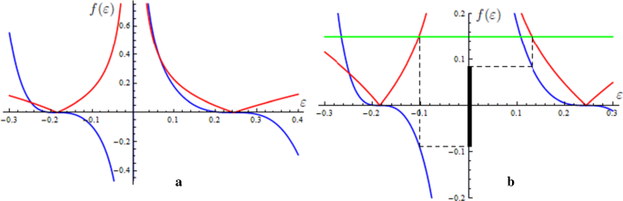

  

  Geometrical interpretation of conditions (49)

  The proposed procedure is easy to explain using a geometric representation. Figure 7a shows the curves $C_1: f_1 = h_{\mathrm{hyst}} (\varepsilon ), \ C_2: f_2 = 50 \varkappa _{\mathrm{hyst}} (\varepsilon )$. For given value of $h_0 = 0.15$ (Fig. 7b) we determine the values of $\varepsilon : \varepsilon _1 \approx -0.103, \ \varepsilon _2 \approx 0.147$—the points of intersection the line $f = h_0$ and curve $C_1$. After that we find the values $f_2 (\varepsilon _1), f_2 (\varepsilon _2).$ With this we have determined the interval of safe values for $50 \varkappa$ as $(-\,0.088, 0.083)$. Since, according to formulas (3), $\varkappa$ depends on $F_0$, then we obtain the corresponding interval for $k_a ^{\mathrm{nonlin}} \approx (-\,0.258, 0.027)$. These results correlate with ones of paper [17] which are presented in Fig. 2. (They are not completely identical, because in [17] the primary system has nonlinear stiffness component.)

• (B) $\frac{\partial ^2 g}{\partial \rho ^2} \ne 0, \ \frac{\partial g}{\partial \varepsilon } = 0$. The possibility of other types of bifurcation can be analyzed in same manner. Although the explicit formulas for $\varepsilon , \rho$ cannot be obtained, the numerical analysis is simple enough. In particular, for the values from table 1, there are two points of simple bifurcation ($\varepsilon \approx -\,0.055, \varkappa \approx -\,0.00100, \rho \approx 183.17$ and $\varepsilon \approx 0.060, \varkappa \approx -\,0.00095, \rho \approx 203.90$).

4 Analytical estimation of the responses and tuning the NDVA

The magnitude of the responses of the main mass is determined by function $\sqrt{ u_1 ^2 (\tau ) + v_1 ^2 (\tau )}.$ If the stationary point $M_0 ({\varvec{u_0, v_0}})$ is an attractor, then after the first phase of the motion (restructuring of trajectory after receiving the initial perturbation), this function tends to $\sqrt{u_ {10} ^ 2 + v_ {10} ^ 2}.$ In mathematical formulation, this aspiration occurs as $t \rightarrow \infty$. In fact, after a certain period of time $I_1 = [0, \tau _1 ]$ the phase trajectory falls into some sufficiently small neighborhood of the point $M_0$. Therefore, the problem of mitigation the oscillations of the main system can be formulated as a problem of minimizing the magnitude of $\sqrt{u_ {10} ^ 2 + v_ {10} ^ 2}$ with the additional condition that the value of $\tau _1$ is not too large. For technical reasons, it is more convenient to choose

$$\begin{aligned} \xi (h,\gamma , \varkappa , \mu , \varepsilon ) \triangleq u_{10} ^2 + v_{10} ^2 \end{aligned}$$

(50)

as the target function. Values of $u_{10}, v_{10}$ are yielded by the system (14) through $u_{20}, v_{20}$, and $u_{20}$ is estimated by $v_{20}$ according to the formula (20). Finally, $v_{20}$ is the root of the cubic equation (21). The roots of this equation can be written down explicitly using the Cardano formula. However, this solution contains the roots of the second and third degrees and depends on the five parameters $\mu , \varepsilon , h, \gamma , \varkappa .$ Therefore, it is completely unsuitable for further analysis. For this reason, we suggest the following procedure.

With fixed values of the parameters $h = h_ *, \ \gamma = \gamma _ *, \ \varkappa = \varkappa _ *, \ \mu = \mu _ *, \ \varepsilon = \varepsilon _ *,$ the value of $v_ {20}$ is defined as a root of the polynomial $P_1$ and, being substituted [taking into account the formulas (20), (14)] into (50), gives the corresponding value $\xi _ *.$ Since $\xi$ can be considered as a polynomial $P_4$ with regard to $v_2$ and with coefficients depending on the parameters

$$\begin{aligned} P_4 (v_2) & = b_{12}^4 \varkappa ^2 v_2 ^4 + 2 h \varkappa b_{12}^3 (b_{11} v_2 ^3 b_{22} - b_{12}^2)\nonumber \\&\quad+\, h^2 b_{12}^2 v_2 ^2 [ h^2 b_{11}^2 - 2 \varkappa b_{11}^2 \nonumber \\&\quad+ \,(b_{11} b_{22} - b_{12}^2 )^2 ] \nonumber \\&\quad- \,2 h^3 b_{11} b_{12} v_2 (b_{11} b_{22} - b_{12}^2 ) + h^4 b_{11}^4, \end{aligned}$$

(51)

then $\xi _*$ satisfies the system $P_1 (v_2) = 0, \ P_4 (v_2) = 0$, that is, is the root of the following polynomial

$$\begin{aligned}&P_5 (\xi ) \triangleq res(P_1, P_4, v_2)\nonumber \\&\quad = - \varkappa ^2 b_{11}^2 \xi ^3 + \varkappa b_{11}^3 b_{12}^2 \xi ^2 [ 3 \varkappa b_{11} + 4 h^2 b_{11}^2 \nonumber \\&\qquad + \,2 b_{12}^2 (b_{11} b_{22} - b_{12}^2 )]\nonumber \\&\qquad - \,\xi \{ 3 \varkappa ^2 b_{11}^2 b_{12}^4 + 2 b_{11} b_{12}^4 (4 h^2 b_{11}^2 + 3 b_{12}^4) \nonumber \\&\qquad +\, b_{12}^4 [4 h^4 b_{11}^4 + h^2 b_{11}^2 (4 b_{11}^2 b_{22}^2 - 8 b_{11} b_{12}^2 b_{22}\nonumber \\&\qquad + \,5 b_{12}^4) + b_{12}^4 (b_{11} b_{22} - b_{12}^2 )^2 ] \}\nonumber \\&\qquad + \,b_{12}^6 [ \varkappa ^2 + 2 \varkappa (2 h^2 b_{11} - b_{12}^2 b_{22}) \nonumber \\&\qquad + \,4 h^4 b_{11}^2 + h^2 (4 b_{11}^2 b_{22}^2 + b_{12}^4) + b_{12}^4 b_{22}^2] . \end{aligned}$$

(52)

After substitution of expressions for $b_ {11}, \ b_ {12}, \ b_ {22}$ [formulas (13)] the resulting formula is rather cumbersome to be given here.

Since, by assumption, the ratio $\varOmega _0 = \omega / \tilde{\omega }_1$ is close to 1, we can assume that $\varepsilon \ll 1,$ and the specific magnitudes of $m_1, k_1,$ as well as the ranges of varying of $\omega , F_0,$ are known when setting the task for a given mechanical system (1). It is also obvious that the efficiency of the absorber is the higher, the greater its mass. At the same time, due to constructive considerations, there is usually a top limit on the value $m_a$, that is, we can assume that the value of the parameter $\mu$ is known (for a particular system). Thus, the task is to find such parameters $\gamma , h, \varkappa$ (tuning of the absorber), at which the maximum on $\varepsilon$ of the function (46) takes the smallest value.

In principle, this problem can be solved numerically, but such a solution can have serious errors, since the limits of variation of various parameters differ significantly. As will be shown below, there is a “very small” order parameter ($10^{-5}$), small order ($10^{-1} {-} 10^{-2}$) parameters and a large order ($10^3 {-} 10^4$) parameter. Therefore, to find the optimal configuration of the absorber, we propose the following combined numerical-analytical approach. For a given value of $\mu$ as a first approximation for $h, \gamma$ we take the same values as in the case of a linear absorber, using known formulas ([3, 48] or the like). For instance, according to [3] we have the following formulas

$$\begin{aligned} \omega _a = \frac{\omega _1}{(1 + \mu ^2)}, \ \frac{c_a}{m_a \omega _1} = \sqrt{\frac{3}{2}} \frac{\mu }{(1 + \mu ^2)^{3/2}}, \end{aligned}$$

(53)

which imply the following estimations: $\gamma _{\mathrm{DH}} \approx -0.01, \ h_{\mathrm{DH}} \approx 0.12 \ (\mu = 0.1)$. Constructing the surface $P_5 (\xi , \varepsilon , \varkappa ) = 0$, we can make a decision about the appropriate range of the parameter $\varkappa$.

Figure 8a displays the parameter $\varkappa$ range is taken $[-\,0.1,0.1]$. It is clear that such range is too large, because in the middle of the surface there is a notch in which the values of $\xi$ are much less than 4000. In Fig. 8b this range is reduced of a hundred times, and, obviously, it should be further reduced in order for the peaks at the edges of the pattern to disappear. In Fig. 8c there is no strong change in the height of the upper edge, and a rough estimate of the size can be made as $\varkappa \in [-\,0.00007,-\,0.00005]$.

Fig. 8

Delimitation of the appropriate range for parameter $\varkappa \ (\mu =0.1)$

Fig. 9

Refinement of the first approximation

Now, taking as a first approximation $\gamma = -0.01, \varkappa ^{(1)} = -0.6 \times 10^{-4}$, we vary $h^2$ within such limits so as $\xi$ not to exceed value $\approx 210 - 220$. In such a way we determine the amendment to the taken value: $hh_1 = (h^{(1)})^2 \approx 0.015$ (Fig. 9a) instead of $h_0 ^2$. Substituting $hh_1$ in (52), we vary $\gamma$ (Fig. 9b). After that, the values found are refined from the condition of equal peaks at the lowest possible value of $\xi$ (Fig. 9c). Thus, the values found are $\gamma = - 0.0153, hh = 0.015, \varkappa = -0.52 \times 10^{-4}$.

Verifying the correctness of the result can be easily performed using the expression (52). If there is a set of values $\gamma _{\star }, h_{\star }, \varkappa _{\star }$ for which $\xi$ takes a value less than that found (for example, $\xi _1 = 201.1$), then the straight line $\xi = 201$ intersects the curve $P_5 (\xi , \gamma _{\star }, h_{\star }, \varkappa _{\star }, \mu , \varepsilon ) = 0$ at four points, that is, the polynomial $P_5 (\xi , \varepsilon )\mid _{\xi = 201}$ has four real roots on the interval $[\varepsilon _1, \varepsilon _2]$. If this equation has two roots $\varepsilon ^{(1)}, \varepsilon ^{(2)}$ for any $(\gamma _{\star }, h_{\star }, \varkappa _{\star })$ from the region $D_{\mathrm{par}}$, and $\varepsilon ^{(1)} \cdot \varepsilon ^{(2)} > 0$, then this means that at a certain frequency of external excitation $\omega _{\star }$, such that $\varepsilon _{\star } \in (\varepsilon ^{(1)}, \varepsilon ^{(2)})$ the corresponding value $\xi _{\star }$ exceeds the value $\xi = 201$.

Remark 4.1

Of course, if the polynomial $P_5 (\xi , \varepsilon )\mid _{\xi = 201}$ does not have real roots on the interval $(\varepsilon ^{(1)}, \varepsilon ^{(2)})$ for some set $(\gamma _{\star }, h_{\star }, \varkappa _{\star })$, this means that the straight line $\xi = 201$ passes above the peaks, that is, for these values we have $\xi _{\star } < 201$, and the parameters found $( -\,0.0153, 0.015, -\,0.52 \times 10^{-4}$ in our case) need to be revised.

Remark 4.2

If there are two real roots, but, $\varepsilon ^{(1)} \cdot \varepsilon ^{(2)} < 0$, this means that two peaks are involved in, then a set of parameters $(\gamma _{\star }, h_{\star }, \varkappa _{\star })$ has been found for which we have the equality of the peaks. Such a situation is possible from a mathematical point of view, although it can be numerically realized only with some accuracy limit specified in advance.

Summarizing the content of this section, we believe that methodology suggested allows to reduce the range for search of the appropriate values for nonlinear component of stiffness. A possible alternative approach is to solve the optimization problem by a grid search. However, in a multidimensional model space, such approach will be computationally more expensive and scales as $N^d$, where d stands for the dimensionality of the problem. For example, the given problem has four free parameters to optimize $(d = 4)$. Given the high sensitivity of the function to the parameters, the number of evaluations per grid direction N will be in the range of at least several tens. Thus, the total number of function evaluations required to achieve the desired optimization accuracy using the grid search can be in the range of hundreds of thousands.

5 Numerical analysis

In this section, the case studies are inspected to check the performance of the absorber attached to primary oscillator. The responses of the system obtained from analytical approximations, which are based on the averaging method, are compared with numerical integrations based on a fourth-order Runge–Kutta method. In order to facilitate the comparison with the results of Sects. 3 and 4, we use dimensionless parameters and variables introduced according to the formulas (3).

5.1 Comparing the behavior of the trajectories of systems (9) and (11)

First, we compare the results of the numerical integration of the equations of the motion and the averaged ones. Namely, we check how well the information obtained from the analysis of the averaged equations corresponds to the behavior of the solutions of the original mechanical system. The values of the parameters were taken as follows: two values for $\mu$ were taken in turn, namely 0.1 and 0.14, parameters $\gamma , h, \varkappa$ are ranging from $-\,0.2$ to 0.2, from 0.05 to 0.5, and from $-\,0.001$ to 0.001, respectively.⁴ The frequency ratio was varying from 0.5 to 1.5, though the peaks of the responses are situated closer to 1. For chosen values of parameters $\gamma , h, \varkappa$ the distance between peaks is proportional to $\mu$ and at first approximation is close to $2 \mu$.

Fig. 10

The motion of main mass: a time interval $\tau \in [0, 50]$; b, c$\tau \in [50, 150]$, the dot line corresponds to averaged equations ($\mu = 0.1, \varepsilon = - 0.02, \gamma = - 0.015, h = 0.14, \varkappa = 10^{-4})$

Fig. 11

Time histories related to Fig. 10 (a, b); motion of the absorber for $\tau \in [0, 100]$ (c)

Figures 10 and 11 show projections of typical phase trajectories on the planes $O u_1 v_1$ (the primary system) and $O u_2 v_2$ (the absorber). Figure 10a exhibits the projections of the phase trajectory of the system (9) (solid curve) and averaged Eq. (11) (dot curve). The following initial values are taken: $u_1 (0)= 8, v_1 (0) =-3$, $u_2 (0) = -2.5, v_2 (0) = 3,$ and the time interval is $\tau \in [0, 50]$. In Fig. 10b, c, the same trajectories are shown separately within the time interval $\tau \in [50, 150]$. Fig. 11 shows the time histories of the components $u_1 (\tau ), v_1 (\tau )$ (Fig. 11a, b), as well as the behavior of the absorber (Fig. 11c). Two circumstances should be noted in this regard. The first is that the absorber calms down ostensibly faster than the main mass (compare Figs. 10b and 11c). In fact, this is not so—we recall that the variable $\widetilde{x}_2$ and, consequently, $u_2, v_2$ are taken with a multiplier $\mu$ [see formula (4)], so the absorber responses are 10 times more than those shown in the figure. The second circumstance concerns the time histories of coordinates $u_j, v_j \ (j=1,2)$ for the complete system of Eq. (9) and the averaged curve shown in Fig. 11. As one can see, the points belonging to the dashed curve accurately reflect the behavior of the function

$$\begin{aligned} \hat{v}_1 (\tau ) = \frac{1}{T} \int _0 ^{\tau } v_1 (t_1) {\hbox {d}} t_1 \end{aligned}$$

(54)

(the same situation holds for $u_2 (\tau ), v_2 (\tau )$, although they are not shown in the Figure). In the case of the variable $u_1$, we see some discrepancy, i.e., the curve corresponding to the averaged equations follows the lower edge of the “true” curve $u_1 (\tau )$. This discrepancy is explained by the fact that the first equation of the system (9) contains a term $\sin 2 \tau$ that is of order 1, but it disappears with averaging (observe that for other equations of the system, this does not occur).

Fig. 12

Attraction of the phase trajectories to the fixed point of system (11) for different initial perturbations: a time interval $\tau \in [0, 100]$, b time interval [100, 130] ; attractors for system (9) with initial values: $(8, -\,2.5, -\,3, 3)$ for case (c) and $(6, 5.5, -\,5, 0)$ for case (d)

Finally, Fig. 12 shows that the trajectories of the system are tightened to the attractor. In the case of averaged equations, this attractor, according to the results of Sect. 3, is the fixed point (stable focus), and the trajectories are pulled to this point regardless of the choice of initial values (of course, taking into account restrictions on the magnitude of initial perturbations). Three different paths are shown in Fig. 12a, which, as can be seen in Fig. 12b, after a certain period of time enters a small neighborhood of a point $M_0 (u_{10}, v_{10}, u_{20}, v_{20})$. As for Eq. (11), here the limit cycle is an attractor (Fig. 12c, d), that is, the solutions from a certain neighborhood of the point $M_0$ are asymptotically periodic.⁵ As one can see, the shape of this limit cycle is close to the cardioide with the parameter $a \approx 0.5$.

Remark 5.1

Here and further, commenting on the figures, we say “a limit cycle” for brevity. Of course, we are talking about projections of the limit cycle in 4-dimensional space onto the planes $O u_1 v_1$ and $O u_2 v_2.$

It is obvious that the limits of applicability of the averaging method (in general) and for this problem (in particular) are bounded. Consider as an illustration the case when Eq. (22) has three real roots. To find the appropriate values of the parameters, we can use the inequalities (23) (or Fig.3). Choosing $\mu = 0.1, \gamma = -0.01, h = 0.01,$ it follows from the Fig. 3d that we can take, for example, $\varepsilon = -0.01, \varkappa = -2 \times 10^{-4}$. Substituting the latter values into (31), we have $\sigma _1 \approx -0.02957, \ \sigma _2 \approx -\,0.7709, \ \sigma _3 \approx -\,1.1017$. For a smallest absolute value of sigma, dynamics is predicted by the used averaging procedure. For the averaged system (11), the trajectory tends to the limit point $M_{01} (- \,23.12, -\, 10.44, 10.90, 11.24)$, whereas for the full system it is attracted to the limit orbit. However, a fundamental discrepancy already exists for the values $\sigma _2, \sigma _3$. For the averaged system, the corresponding stationary point is an attractor (stable focus). For instance, with $\sigma = \sigma _2$ Eq. (28) has two pairs of complex conjugate roots $-\,0.005 \pm 0.666 i, \ -\, 0.273 \times 10^{-4} \pm 0.898 \times 10^{-2} i$, respectively, and the damping rate is very weak (Fig. 13a). However, the trajectory corresponding to Eq. (9) behaves differently (Fig. 13b, c). This is because the amplitude of the oscillations of the main mass is too large ($M_{02} (- \,512.56, -\, 63.02, 39.89, 4.11)$), and the amplitude of each individual pulse is also large (Fig. 13b).

Fig. 13

Dispersal of phase trajectories of the averaged equations (11) (a) and the authentic ones (9) (b, c) for large initial values. The scaling factor is 1:40

Fig. 14

Discrepancy in behavior of phase trajectories at the beginning of the motion: averaged system (a, c); original system (b, d)

Figure 14 reports in more detail the initial phase of the perturbed motion. As one can see, from the very beginning the trajectory corresponding to the averaged equations does not reflect the behavior of the trajectory of the system (9) (compare Figs. 11b and 14d).

5.2 Influence of the DVA nonlinear stiffness component

This subsection describes some of the features inherent in the nonlinear component $k_a ^{\mathrm{nonlin}}$, which is an important part of tuning of the DVA and it has been presented in our studying through the parameter $\varkappa$. As it follows from Sect. 4, in the case of a “one-sided” frequency range ($\varepsilon _1 \varepsilon _2 > 0$)⁶ a softening spring should be taken when $\varOmega _0 < 1$, and a hardening spring in opposite case. This conclusion is confirmed by numerical calculations. The magnitude of the parameter $\varkappa$ is determined according to the procedure described in Sect. 4 and is influenced by mass ratio and frequency range.

Fig. 15

Influence the magnitude of parameter $\varkappa$ onto amplitude of the oscillations [$\tau _1 \in [180, 600]$ (a), $\tau _1 \in [800, 1400]$ (b), $\tau _1 \in [1600, 1660]$ (c)]

For low frequencies ratio ($\varepsilon < 0$), one deals with a softening spring, and gradual increase in the parameter $\varkappa$ values from zero to a certain limit helps to reduce the amplitude of the oscillations (Fig. 15a, $\varkappa (1) = 0, \ \varkappa (6) = -0.7\cdot 10^{-4}$). It should be noted that for curves 5, 6 as compared with 2,3, the amplitude decreased by $30 {-} 35 \%$. At the same time, the duration of the transition process has doubled and more. Meanwhile, a further increase in the magnitude of $\varkappa$ leads to a change in the qualitative picture. Namely, the beats appear (Fig. 15b), and the transition time to the limiting cycle increases significantly (another 2–3 times). The further growth in $\varkappa$ leads to instability regime. Although in the left part of the Fig. 15c the amplitude of oscillations is low, but in the right part it is higher than the counterpart shown in Fig. 15a (the curves 5, 6).

The following interesting feature has been detected: when changing the parameter $\varkappa$, the shape of the limit cycle for the main mass almost does not change (or changes insignificantly with a significant (several times) increase in the parameter module). At the same time, the shape of the limit cycle for the absorber has been greatly modified. Our numerical experiments have yielded three qualitatively different forms: (A) a “crumpled” cardiode; (B) a “loop” (“figure of eight”); (C) a “triangle” (Fig. 16).

Fig. 16

Evolution the shape of the limit cycle for DVA under increasing value of $\varkappa$

If the frequency interval is two-sided ($\varepsilon _1 \varepsilon _2 < 0$), then it is advisable to use a hardening spring, and the $|\varkappa |$ should be taken 8–10 times smaller in comparison with the previous case. For this reason, the amplitude of oscillations, generally speaking, increases, including for positive values of $\varepsilon$, but this is a kind of compensation to protect the primary system against much greater growth of oscillations amplitude with possible negative values $\varepsilon$.

Also, the following important circumstance should be taking into account. As noted above, one of the key points of this paper is based the assumption that the parameters of the main system and the external excitation are uncertain. That is, when solving the problem of setting up the device to reduce oscillations of a particular mechanical system, we can assume that the quantities $m_1, k_1, \varepsilon _1, \varepsilon _2,$ (and $m_a$) are known. At the same time, unlike $\gamma , h$, the parameter $\varkappa$ depends significantly on $F_0$. If its magnitude is known accurately enough, then the value of $\varkappa$ is easily transformed into a value for $k_a ^{\mathrm{nonlin}}$, as predicted. However, a situation may appear when the interval $[ F_1, F_2]$ of a possible change of $F_0$ (within the framework of one task) is not narrow; say $F_2$ is of 5–10 times more than $F_1$. In this case, to determine the value of $k_a ^{\mathrm{nonlin}}$ one should take the maximum value for F, that is,

$$\begin{aligned} k_a ^{\mathrm{nonlin}} = \frac{4}{3} \frac{k_1 m_a ^2}{\varkappa m_1 ^2 F_2 ^2}. \end{aligned}$$

(55)

For this reason a significant decrease in “hardening ability” of the spring may occur, which leads to some degradation of the absorber effectiveness. However, if we take some “more neutral” value, for instance $(F_1 + F_2 ) / 2$, and $F_2 = 5 F_1$ then, in case $F_0 = F_2$ we have the quadruple increase in value for $|\varkappa |$, and this may lead to much more increase in amplitude of the responses of primary system (see Fig. 15).

5.3 Tuning the DVA and numerical validation

Now we check the recommendations regarding the choice of absorber’s parameters based on the numerical integration of Eqs. (9) and (11). We consider that the mass of the absorber and the interval of possible values of the frequency of external influence are known: $\mu = 0.14, \ \varepsilon \in [-\,0.15, 0.2]$. As can be seen from Fig. 8, in this case the surface has two ridges, that is, the amplitude-frequency curve has two peaks. Performing the appropriate calculation, we obtain the following values $\gamma \approx - 0. 022, h^2 \approx 0.028, \varkappa \approx - 0.54 \times 10^{-4}$. The corresponding value of function $\xi$ in this case is $\approx 104$. Substituting the values of the parameters and the initial values $u_1 (0) = 7, v_1 (0) =-6, u_2 (0) = - 0.5, v_2 (0) = 1$, we build the phase portrait, and the projections of limit cycles onto the plane $O u_1 v_1$ are shown in Fig. 17a, b. These cases correspond to two peaks related to the system (11). The coordinates of the point $M_0$ obtained by solving the system (14) are $( 6.72, 7.46, -\, 2.56, 6.17)$ for $\varepsilon = -0.1$ (the left peak) and $( -\, 4.67, 9.10, -\,3.12, -\,6.68)$ for $\varepsilon = 0.11$ (the right peak).

Fig. 17

Maximum responses of the primary mass for different values of $\varkappa$

Note that a slight change in the selected parameters does not affect the magnitude of the maximum responses too much, although it may worsen some of the secondary characteristics. For example, in Fig. 17b, the time of the transition period (the time during which the trajectory reaches a small neighborhood of a stationary point) is $\approx 90\,\mathrm{s}$ (on $\tau$-scale), and in Fig. 17c—$\approx 105\,\mathrm{s}$. Recall also that $\gamma$ is a detuning parameter of the linear component of the stiffness of the absorber relative to the stiffness of the main mass. Therefore, a change in $k_a ^{\mathrm{lin}}$ of $1{-}2 \%$ corresponds to a change of $50{-}100 \%$ for $\gamma$, and this component is the most vulnerable link in terms of tuning accuracy. Changing the parameter h characterizing the damping, say $10 \%$, does not matter much (Fig. 17c). The most “vigorous” role plays the nonlinear component of stiffness. In Fig. 17d–f there are presented limit cycles for three different values of $\varkappa :$ weaker the sample one ($-\,0.3 \times 10^{-4}$ against $-\,0.54 \times 10^{-4}$) and two other ones for values $- \,10^{-4}$ and $-\,2 \times 10^{-4}$. Even the increasing the absolute value of the magnitude of this component at four times leads to rather little increase of the amplitude of oscillations of primary system.

However, such a flexible nature of the coefficient $\varkappa$ does not apply to a change in its sign. The change of its value from $-\,0.3 \times 10^{-4}$ to $0.3 \times 10^{-4}$ makes the difference. At the frequency of the former peak $\varepsilon = 0.11$), the amplitude of oscillations does not increase (Fig. 17g). However, when frequency ratio changes a little ($\varepsilon = 0.12$), the motion becomes unstable (Fig. 17h).

Fig. 18

$\varOmega _0$ as frequency ratio: the geometrical viewpoint

5.4 On the choice of the frequency ratio

The term “frequency ratio”, apparently, was used by Dan Hartog [3] firstly in order to denote the ratio of the frequency of an external excitation to the frequency of the main mass. This designation is natural, understandable and generally accepted. At the same time, although we are talking about the dynamics of the “main mass + absorber” system, this value does not reflect the influence of the latter. For this reason, it seems to us that more natural for “frequency ratio” is the expression $\varOmega _0 = \varOmega / (1 + \mu ^2)$, which represents the ratio of the frequency of an external force to the frequency of the main system with additional mass $m_a$ (“frozen” absorber). Of course, usually the mass of the absorber is small compared to the main mass, and the difference between $\varOmega$ and $\varOmega _0$ is quite small. However, we see the following arguments in favor of preference $\varOmega _0$ before $\varOmega .$

• (1) Referring to the surface view $P_5 (\xi ) = 0$ which at each point in the region $D_{\mathrm{par}}$ determines the value of the square of the amplitude of the responses of the main system. Recall that according to the formulas (3), the value corresponding to $\omega _0$ is $\varepsilon =0$, and the value for $\omega _1$ is $\varepsilon = \mu ^2 / (1 + \mu ^2 )$. As we see from Fig. 18, the plane $\varepsilon = 0$ passes through the “vale” of the surface (Fig. 18a, b), in the plane it is very close to the minimum of the function $\xi ( \varepsilon )$ (Fig. 18c).

• (2) Another point arises from an analytical reason. According to Sect. 2, with $\varepsilon = 0$ the system (11) has a single stationary point for any set of parameters of the absorber. For nonzero value of $\varepsilon$, as can be seen from the Fig. 3, there are configurations of the DVA which bring three stationary points into consideration. Thus, the zero value for $\varepsilon$ logically may be considered as starting point for various analytical constructions (the perturbation theory for instance).

• (3) Frequently, the authors divide the frequency range of $\omega$ by using the $\omega _1$ as a border and the low frequencies ($\varOmega < 1$) and high frequencies ($\varOmega > 1$) as dividing values. The subsequent analysis is carried out taking into account this partition. For instance, in [14] the authors analyze the effect of a nonlinear absorber on a linear basic system and give the conclusion: “In the low-frequency range of $\varOmega < 1$, a softening stiffness absorber performs well by increasing power absorption ratio and reducing peak. ...In comparison, the hardening stiffness absorber enhances power absorption and attenuates the peak of kinetic energy in the high-frequency range of $\varOmega > 1$.” We believe, that such conclusion will be more accurate by replacing $\varOmega$ with $\varOmega _0$. We consider the following examples to validate our statements.

Example 5.1

Let the mass ratio is $m_a / m_1 = 0.0196 \ (\mu =0.14)$, and the frequency range is $\varepsilon \in (-\,0.2, 0) \ (\varOmega _0 < 1)$. In this case a softening spring ($\varkappa > 0$) is preferable. Since the amplitude curve has only one peak, it is necessary to minimize the largest of the values $\xi (\gamma , h, \varkappa )|_{\varepsilon =-0.2}$, $\xi _{\mathrm{max}}(\gamma , h, \varkappa ), \ \xi (\gamma , h, \varkappa )|_{\varepsilon = 0}.$ Taking into account that $\frac{\partial \xi }{\partial \varepsilon }|_{\varepsilon =-0.2} > 0$, two values need to be compensated, i.e., the peak value and its counterpart at the right border of the interval.

The ranges for parameters $\gamma , h, \varkappa \$ we determine according to approach described in Sect. 4. Thereafter the optimal values are determined by simple procedure which is illustrated in Fig. 19. Now taking $\gamma = -0.094, \ h = 0.095, \ \varkappa = 0.9 \times 10^{-4},$ we plot the frequency–amplitude curve (Fig. 20a). The maximum value is $\xi _{\mathrm{max}} \approx 52.3$. From the other side, counting the right border as $\varepsilon = 1 - 1 / (1 + \mu ^2) \approx 0.0192$ and optimizing the parameters, we get another curve which gives the bigger value for $\xi : \approx 65.2$.

Fig. 19

Inspection of possible candidates: for given value of $\gamma$ different pairs of $h, \varkappa$ are tested [the solid symbol is related to the peak value of $\xi$, and empty symbol is related to the right border value of $\xi (0)$]

Example 5.2

Another possibility to compare two candidates $\omega$ and $\omega _0$ is the testing of the debatable interval $[ \omega _0, \omega ]$ or $I_{\varepsilon } = [0, 1 / (1+\mu ^2) ]$. If one choose $\omega$ as a borderline, this is a low-frequency range, and a high-frequency range with the choice of $\omega _0$. At the first case we have to take the softening stiffness ($\varkappa > 0$) and the hardening stiffness in opposite case. Figure 20 presents the frequency–amplitude curves (Fig. 20b) and the results of integrating the motion equations for both cases (limit cycles in Fig. 20c). Thus, the hardening spring gives about $25\%$ lower amplitude of the responses.

Fig. 20

Comparison of two options: $\varOmega _0$ (a, b—solid curve) and $\varOmega$ (dashed curve)

6 Concluding remarks

We have studied the problem of determining the parameters of NDVA in order to reduce the maximum possible amplitude of oscillations of the main system in the conditions of uncertainties (frequency ratio and amplitude of external excitation). Particular attention is paid to the development of an analytical procedure that allows to easily algorithmize the procedure for setting up the absorber and testing the results obtained. The influence of the nonlinear elastic characteristic of DVA on the efficiency of work is studied, the recommendations are given on the choice of the spring (hardening or softening) depending on the expected frequency ranges and the amplitude of the external influence. The necessary and sufficient conditions for the asymptotic stability of the quasi-periodic motions of the mechanical system under study are found based on the use of a simplified mathematical model (the averaged equations). Technically, the proposed approach may be described by the following scheme shown in Fig. 21.

Fig. 21

Scheme of the developed technique

The validity of using such a model is confirmed by the results of numerical experiments. The approach used in the article can be extended to cases of a nonlinear main system and a system with many degrees of freedom.

Finally, we emphasize importance of our study. Namely, under conditions of uncertain parameters, the direct numerical optimization can be inefficient or at least costly. This is because for this problem there is no explicit expression for the objective function, moreover, it is a function of many $(\ge 4)$ variables, some of which are tougher (a small change weakly affects the behavior of the system), while other parameters are very sensitive (linear and nonlinear absorber stiffnesses). In this work, to set up the absorber, an approach based on visualization is used an image in the form of a surface of the dependence of the oscillation amplitude of the main system on the frequency and nonlinear component (nl.c.) of the absorber stiffness. This allows with easy localize the interval of suitable values for nl.c. After that, the remaining parameters are refined. Localization of the interval for nl.c. seems to be an important step, since initially this parameter is completely undefined (in dimensionless parameters, the appropriate values appear of the order of $10^{-5}$, so iterating over possible values with a step 0.01, for instance, will be ineffective.

The mathematical expression for the objective function is rather cumbersome (and the function is specified implicitly), but computer algebra helps to carry out the necessary analysis.

References

Frahm, H.: Device for damping vibrations of bodies (1911). US Patent 989958
Ormondroyd, J., Den Hartog, J.P.: Theory of the dynamic vibration absorber. Trans. Am. Soc. Mech. Eng. 50, 9–22 (1928)
Den Hartog, J.P.: Mechanical Vibrations. McGraw-Hill, New York (1934)
Brock, J.E.: A note on the damped vibration absorber. Trans. ASME J. Appl. Mech. 13, A-284 (1946)
Roberson, R.E.: Synthesis of a nonlinear dynamic vibration absorber. J. Frankl. Inst. 254, 205–17220 (1952)
Gendelman, O.V.: Transition of energy to a nonlinear localized mode in a highly asymmetric system of two oscillators. Nonlinear Dyn. 25, 237–17253 (2001)
Vakakis, A.F., Gendelman, O.: Energy pumping in nonlinear mechanical oscillators: part II 17resonance capture. Trans. ASME J. Appl. Mech. 68, 42–1748 (2001)
Zhu, S.J., Zheng, Y.F., Fu, Y.M.: Analysis of non-linear dynamics of a two-degree-of-freedom vibration system with non-linear damping and non-linear spring. J. Sound. Vib. 271, 15–1724 (2004)
Gendelman, O.V., Starosvetsky, Y.: Quasi-periodic response regimes of linear oscillator coupled to nonlinear energy sink under periodic forcing. J. Appl. Mech. 74, 325–17331 (2007)
Jing, X.J., Lang, Z.Q.: Frequency domain analysis of a dimensionless cubic nonlinear damping system subject to harmonic input. Nonlinear Dyn. 58, 469 17 485 (2009)
Viguié, R., Kerschen, G.: Nonlinear vibration absorber coupled to a nonlinear primary system: a tuning methodology. J. Sound. Vib. 326, 780–17793 (2009)
Petit, F., Loccufier, M., Aeyels, D.: The energy thresholds of nonlinear vibration absorbers. Nonlinear Dyn. 74(3), 755 17 767 (2013)
Kremer, D., Liu, K.: A nonlinear energy sink with an energy harvester: transient responses. J. Sound. Vib. 333(20), 4859–174880 (2014)
Yang, J., Xiong, Y.P., Xing, J.T.: Power flow behaviour and dynamic performance of a nonlinear vibration absorber coupled to a nonlinear oscillator. Nonlinear Dyn. 80(3), 1063 17 1079 (2014)
Casalotti, A., Lacarbonara, W.: Nonlinear vibration absorber optimal design via asymptotic approach. IUTAM Symp. Anal. Methods Nonlinear Dyn. Proc. IUTAM 19, 65 17 74 (2016)
Taleshi, M., Dardel, M., Pashaie, M.H.: Passive targeted energy transfer in the steady state dynamics of a nonlinear plate with nonlinear absorber. Chaos Solitons Fractals 92, 56–72 (2016)
Cirillo, G.I., Habib, G., Kerschen, G., Sepulchre, R.: Analysis and design of nonlinear resonances via singularity theory. J. Sound Vib. 392, 295–306 (2017)
Lee, Y.S., Kerschen, G., Vakakis, A.F., Panagopoulos, P., Bergman, L., McFarland, D.M.: Complicated dynamics of a linear oscillator with a light, essentially nonlinear attachment. Physica D 204, 41–1769 (2005)
Quinn, D.D., Gendelman, O.V., Kerschen, G., Sapsis, T., Bergman, L.A., Vakakis, A.F.: Efficiency of targeted energy transfers in coupled nonlinear oscillators associated with 1:1 resonance captures: part I. J. Sound Vib. 311, 1228–171248 (2008)
Vakakis, A.F., Gendelman, O., Bergman, L.A., McFarland, D.M., Kerschen, G., Lee, Y.S.: Nonlinear Targeted Energy Transfer in Mechanical and Structural System. Springer, Berlin (2009)
Jo, H., Yabuno, H.: Amplitude reduction of primary resonance of nonlinear oscillator by a dynamic vibration absorber using nonlinear coupling. Nonlinear Dyn. 55, 67–78 (2009)
Starosvetsky, Y., Gendelman, O.V.: Vibration absorption in systems with a nonlinear energy sink: nonlinear damping. J. Sound Vib. 324, 916–17939 (2009)
Ji, J.C., Zhang, N.: Suppression of the primary resonance vibrations of a forced nonlinear system using a dynamic vibration absorber. J. Sound. Vib. 329, 2044–172056 (2010)
Gatti, G., Brennan, M.J., Kovacic, I.: On the interaction of the responses at the resonance frequencies of a nonlinear two degrees-of-freedom system. Physica D 239, 591 17 599 (2010)
Gendelman, O.V., Sapsis, T., Vakakis, A.F., Bergman, L.A.: Enhanced passive targeted energy transfer in strongly nonlinear mechanical oscillators. J. Sound Vib. 330, 1–178 (2011)
Xiao, Z., Jing, X., Cheng, L.: The transmissibility of vibration isolators with cubic nonlinear damping under both force and base excitations. J. Sound. Vib. 332, 1335–171354 (2013)
Bellizzi, S., Côte, R., Pachebat, M.: Responses of a two degree-of-freedom system coupled to a nonlinear damper under multi-forcing frequencies. J. Sound. Vib. 332, 1639–171653 (2013)
Habib, G., Detroux, T., Viguie, R., Kerschen, G.: Nonlinear generalization of Den Hartogs equal-peak method. Mech. Syst. Signal Process. 52, 17–1728 (2015)
Detroux, T., Habib, G., Masset, L., Kerschen, G.: Performance, robustness and sensitivity analysis of the nonlinear tuned vibration absorber. Mech. Syst. Signal Process. 60, 799–17809 (2015)
Taghipour, J., Dardel, M.: Steady state dynamics and robustness of a harmonically excited essentially nonlinear oscillator coupled with a two-DOF nonlinear energy sink. Mech. Syst. Signal Process. 62–63, 164–17182 (2015)
Kremer, D., Liu, K.: A nonlinear energy sink with an energy harvester: harmonically forced responses. J. Sound. Vib. 410, 287–17302 (2017)
Nankali, A., Lee, Y.S., Kalmar-Nagy, T.: Targeted energy transfers for suppressing regenerative machine tool vibrations. J. Comput. Nonlinear Dyn. 12(1), 011010, 1–11 (2017)
Borges, R.A., de Lima, A.M.G., Steffen Jr., V.: Robust optimal design of a nonlinear dynamic vibration absorber combining sensitivity analysis. Shock Vib. 17, 507–17520 (2010)
Nguyen, T.A., Pernot, S.: Design criteria for optimally tuned nonlinear energy sinks-part1. Transient Regime Nonlinear Dyn. 69, 1–1719 (2012)
Jang, S.-J., Brennan, M.J., Rustighi, E., Jung, H.-J.: A simple method for choosing the parameters of a two degree-of-freedom tuned vibration absorber. J. Sound. Vib. 331, 4658–174667 (2012)
Qiu, D., Li, T., Seguy, S., Paredes, M.: Efficient targeted energy transfer of bistable nonlinear energy sink: application to optimal design. Nonlinear Dyn. 92(2), 443–17461 (2018)
Febbo, M., Machado, S.P.: Nonlinear dynamic vibration absorbers with a saturation. J. Sound Vib. 332, 1465 17 1483 (2013)
Carpineto, N., Lacarbonara, W., Vestroni, F.: Hysteretic tuned mass dampers for structural vibration mitigation. J. Sound Vib. 333, 1302–171318 (2014)
Carboni, B., Lacarbonara, W.: Nonlinear dynamic response of a new hysteretic rheological device: experiments and computations. Nonlinear Dyn. 83(117), 23–39 (2015)
Peng, Z.K., Meng, G., Lang, Z.Q., Zhang, W.M., Chu, F.L.: Study of the effects of cubic nonlinear damping on vibration isolations using harmonic balance method. Int. J. Nonlinear Mech. 47, 1073–171080 (2012)
Luongo, A., Zulli, D.: Dynamic analysis of externally excited NES-controlled systems via a mixed multiple scale/harmonic balance algorithm. Nonlinear Dyn. 70(3), 2049–172061 (2012)
Jiang, X., McFarland, D.M., Bergman, L.A., Vakakis, A.F.: Steady state passive nonlinear energy pumping in coupled oscillators: theoretical and experimental results. Nonlinear Dyn. 33, 87–17102 (2003)
Hsu Y.-S., Ferguson N. S., Brennan M.J.: The experimental performance of a nonlinear dynamic vibration absorber. In: Kerschen, G., et al. (eds.), Topics in Nonlinear Dynamics, V.1: Proceedings of the 31st IMAC, Annual Conference on Structural Dynamics, Conference Proceedings of the Society for Experimental Mechanics Series, vol. 35, pp. 241–17257 (2013)
Bronkhorst, K.B., Febbo, M., Lopes, E.M.O., Bavastri, C.A.: Experimental implementation of an optimum viscoelastic vibration absorber for cubic nonlinear systems. Eng. Struct. 163, 323 17 331 (2018)
Mitropolskii, YuA: Method of Averaging in the Investigations of Resonance Systems. Nauka, Moscow (1992). [in Russian]
Lienard, A., Chipart, M.H.: Sur le signe de la partie reelle des racines dune equation algebrique. J. Math. Pures Appl. 10(6), 291 17 346 (1914)
Schaeffer, D.G., Cain, J.W.: Ordinary Differential Equations: Basics and Beyond. Springer, Berlin (2016)
Puzyrov, V., Awrejcewicz, J.: On the optimum absorber parameters: revising the classical results. J. Theor. Appl. Mech. 55(3), 1081–1089 (2017)
Acknowledgements
Funding was provided by Narodowe Centrum Nauki (Grant No. 2017/27/B/ST8/01330).
Author information
Authors and Affiliations
Corresponding author
Ethics declarations
Conflict of interest
The authors declare that they have no conflict of interest.
Additional information
Publisher's Note
Springer Nature remains neutral with regard to jurisdictional claims in published maps and institutional affiliations.
Rights and permissions
Open Access This article is licensed under a Creative Commons Attribution 4.0 International License, which permits use, sharing, adaptation, distribution and reproduction in any medium or format, as long as you give appropriate credit to the original author(s) and the source, provide a link to the Creative Commons licence, and indicate if changes were made. The images or other third party material in this article are included in the article's Creative Commons licence, unless indicated otherwise in a credit line to the material. If material is not included in the article's Creative Commons licence and your intended use is not permitted by statutory regulation or exceeds the permitted use, you will need to obtain permission directly from the copyright holder. To view a copy of this licence, visit http://creativecommons.org/licenses/by/4.0/.
About this article
Cite this article
Awrejcewicz, J., Cheaib, A., Losyeva, N. et al. Responses of a two degrees-of-freedom system with uncertain parameters in the vicinity of resonance 1:1. Nonlinear Dyn 101, 85–106 (2020). https://doi.org/10.1007/s11071-020-05710-7
Received:
Accepted:
Published:
Issue Date:
DOI: https://doi.org/10.1007/s11071-020-05710-7