

Abstract
The microwave cavity perturbation method is widely used for material parameter measurements in connection with small homogeneous samples. Its applicability to larger and inhomogeneous samples is uncertain, but highly desirable in connection with the in-situ condition monitoring of chemical reactors. We have investigated the problem of the reconstruction of axially inhomogeneous permittivity distributions in tubular reactors from measured cavity resonance frequencies of the reactor. It is shown that the use of a priori knowledge about the function class of the permittivity distribution, which in turn follows from assumptions about the chemical process inside the reactor, allows one to reconstruct the permittivity distribution based on a few resonances only. The resulting errors in the function parameters or in the permittivity values identified are on the order of 5%, as demonstrated by analytical and numerical calculations, by numerical experiments, and by laboratory experiments.
Export citation and abstract BibTeX RIS

Original content from this work may be used under the terms of the Creative Commons Attribution 3.0 license. Any further distribution of this work must maintain attribution to the author(s) and the title of the work, journal citation and DOI.
1. Introduction
The in-situ monitoring of chemical reactors is of major interest because a broad range of processes could be operated more efficiently or more safely if the process state were known in more detail. If, for example, the instantaneous oxygen storage level of a three-way catalytic converter in an automotive exhaust gas system were known, emissions could be reduced by well-timed switches between lean or rich operation of the engine [1]. For general chemical reactor processes, several solutions to in-situ monitoring problems have been proposed. Flow injection analysis (FIA) is commercially available and in use in the chemical industry [2]. With this method, samples are injected in a continuous carrier solution and the product resulting from the reaction of sample and solution is run through an analyzer. This procedure is repeated continuously. The time span between two sample injections is chosen in the order of ten seconds. FIA does not allow one to monitor a reactor as a whole, as the samples are drawn from a specific fixed position.
Another common method is Raman spectroscopy. It can be used either as the detector in an FIA system or on its own for direct monitoring [3]. The main drawback is the same as for FIA, viz. only localized analysis is possible.
Microwave imaging, in contrast, can cope with spatial distributions of materials in the reactor. The method responds to spatial variations of the electric permittivity and the electric conductivity inside the reactor. Many details of this approach are still under research. The main issues are long data acquisition times, long computation times, and comparatively large reconstruction errors [4]. This renders microwave imaging unsuitable for in-line process monitoring purposes.
A new approach that has the potential to overcome the problems of the aforementioned existing methods is the use of resonant microwave cavities. A reactor (e.g. a tubular reactor) is closed with metallic grids to form a cavity resonator. The grids let fluids flow in and out of the reactor and simultaneously form a conductive enclosure for microwaves (figure 1). The resonance behavior of the cavity is influenced by the material parameter (permittivity and conductivity) distribution inside. Thus, from the measured cavity resonance behavior one can obtain information about the electrical material parameter distribution (and hence the state of the reaction). In the remainder of the article, 'material parameters' is taken to be short for 'electrical material parameters'.

Figure 1. Schematic drawing of the setup for the proposed measurement method.
Download figure:
Standard image High-resolution imageMaterial parameters have been measured for decades with samples placed in cavities [5–8]. The scattering parameter spectra of the microwave one- or two-ports formed by the cavities, together with appropriate coupling structures, are measured with scalar or vector network analyzers (VNAs). Selected features of these spectra, for example the resonance frequency f0 and the quality factor Q0 of a resonance peak or the average return loss over a given frequency band, are extracted from the spectra. The material parameters of interest are then inferred from the features.
The simplest approach is to fill the cavity completely with a homogeneous material (whole-medium perturbation, WMP) [9]. This allows one to calculate the relative permittivity  and loss parameters (either
  or
or  ) from measured resonance parameters by rather simple equations [10].
Another approach is the small-sample perturbation (SSP) method according to [9]. A small material sample (having a volume of less than about 1% of the cavity volume) is inserted in the cavity. From the difference between the resonance parameters of the unloaded cavity and those of the sample-loaded cavity, the material parameters can be easily calculated (e.g. ch. 6.2.1 in [9]).
Both the uniform large-sample and the small-sample method are well suited for laboratory experiments, but less so for the in-line monitoring of industrial processes. Such industrial processes usually involve inhomogeneous material parameter distributions, which cannot be controlled to satisfy experimental conditions but are dictated by the process. Recently, we have shown that large nonuniform material parameter distributions may be investigated by evaluating multiple resonances in a cavity [9].
A discretized model of an axially inhomogeneous circular cylindrical cavity is shown in figure 2. The continuous material parameter distribution is modeled by a piecewise constant function, i.e. the cavity is treated as if it consisted of N homogeneous segments in the direction of propagation. The actual material parameter distribution is approximated the better by this model, the more segments are used. In the direction perpendicular to the direction of flow (viz. in the radial and azimuthal direction), homogeneity can be assumed with little error in many cases, especially in automotive exhaust treatment systems [11, 12]. We have demonstrated for the case of N = 5 that the permittivities of the five homogeneous segments can be determined on the basis of five measured resonance frequencies [10].
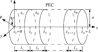
Figure 2. Model of a multi-segment cavity.
Download figure:
Standard image High-resolution imageHowever, this method has its limitations. The inversion algorithm for the inference of the material parameters from the resonance frequencies has convergence issues. It is necessary to carefully choose the start values for the iterative algorithm. A multi-start algorithm can help to find the global optimum [13], but consumes more computing time, which is a decisive drawback in real-time monitoring applications.
Another issue is the sensitivity of the measurement system. On the one hand, this is good for the accuracy of the material parameter measurement, as small changes have a large impact on the resonance frequencies. On the other hand, even small errors in the measured resonance parameters due to, for example, errors of the VNA or a coupling-related cavity detuning have a large impact on the inversion result. This sensitivity to influence quantities is worse for segmented cavities. (It is true in general that the estimation of many parameters is more critical than the estimation of a single parameter. Most ill-posed problems are multi-parameter problems.)
According to [10], three to five segments do not lead to problems. If the errors in the measured resonance parameters are small enough, a few more segments are possible. Even such a coarse discretization suffices to provide valuable information about the instantaneous state of a process which enables one to improve the process efficiency [14].
2. Material parameter distributions in tubular reactors, particle filters, and catalytic converters
The material parameter distribution in chemical reactors (with or without catalyst) or particle filters is a function of the spatial coordinates. We will focus on processes occuring in tubular metal enclosures. The cross-section of the tube can be arbitrary, but usually is circular. For this reason, we limit ourselves to circular cross-sections in the following.
As a consequence of the operation of the reactor, the material parameters in the cavity vary in the axial direction and can be considered constant in the transverse direction. This variation of material parameters is a consequence of a varying concentration of chemical species.
The conversion of a species is described by its reaction order. It describes the influence of the concentration of a species on the reaction rate. For a zeroth-order reaction, the current concentration does not influence the reaction rate at all. The conversion equation for a first-order reaction with a reaction rate constant of k in a tubular reactor is

where X is the conversion of the reactant of interest (negative relative deviation of the local concentration from the starting concentration), Da(z) is the dimensionless Damkoehler number for the reaction at position z, and v is the velocity of flow through the reactor [15].
Assuming losslessness, the resulting permittivity at the reactor input (z = 0) is the effective permittivity of the starting fluid mixture. For ideal mixing, we find [16]
Here,  r, i and ni respectively are the relative permittivity and the mole fraction of the i-th species. There have been published many papers on the issue of fluid mixing, which partially disagree with each other as to what mixing rule is the most appropriate. Reference [17] uses the volumetric fraction instead of the mole fraction. Other, more complex equations were also presented [16, 18]. The following will be based on equation (2).
The relative permittivity of the product after sufficiently long interaction between the various species in the reactor is

By equations (1) through (3), the permittivity distribution along the reactor axis is
where  denotes the amount of substance entering the reactor per unit time (in mol s−1). Inserting (1) into (4) leads to the permittivity distribution resulting from a first-order reaction inside a reactor:

This model equation only involves the three parameters r0, r∞, and k/v. For use in an industrial process, one could measure r0 and r∞ a priori in the laboratory. This would reduce the problem to only one parameter (k/v). If the velocity of flow v is measured additionally, the reaction rate constant k can be determined. This is one key information about a process. Being able to measure this parameter in-line and in real-time, one can control the process better and make it more efficent.
The principle can be applied to other processes if one uses an appropriate permittivity distribution function. Some basic exemplary functions are listed in table 1.
Table 1. Permittivity distribution functions for different processes.
| Model | Permittivity distribution r(z) |
|
|---|---|---|
| No. | Description | |
| 1 | Zeroth-order reaction |  |
| 2 | First-order reaction |  |
| 3 | Second-order reaction |  |
| 4 | Sigmoidal function (propagating reaction front) |  |
3. Measurement method for nonuniformly loaded cavities using model functions
The discretization method described in section 1, by which a continuous material parameter distribution is approximated by a piecewise constant (staircase) function, is no longer applicable when the number N of pieces becomes large. By way of an example, N = 100 would require the measurement of 100 resonance frequencies to determine the (approximated) material parameter distribution. The associated measurement effort, the accumulation of measurement errors when many measured quantities enter into a measurement result, and the sensitivity of the iterative inversion algorithm to these numerical errors all argue against this approach. It is equivalent to finding the global minimum of a function of 100 unknowns based on 100 inaccurate data points. Without measurement errors and with a (vector-valued) start value sufficiently near the solution, the iterative inversion algorithm converges toward the correct solution. Otherwise, and this is the typical process monitoring situation, it finds one of many local minima in the multi-dimensional space of unknowns but may miss the global minimum. In other words, if one aims at the detailed (rather than merely approximate) reconstruction of the spatial variance of material parameters, one needs a different method. Such a method, based on model functions, will be proposed in the following.
3.1. Discretization with model functions
Except for special situations, no closed-form solution of the wave equation for an inhomogeneously loaded cavity is available [19]. The authors of [20] succeeded in deriving a closed-form solution for the E-field of plane waves in unbounded media with a given permittivity distribution, but the effort is considerable. In general, one must tackle the problem numerically, which raises the issue of discretization errors.
For the forward problem, we approximate a continuous permittivity distribution from a given function class (e.g. from table (1) by a staircase function as described in section 1. The mode functions in each segment with homogeneous permittivity distribution are known up to multiplicative scale factors. By enforcing the boundary conditions at the segment interfaces (mode matching), one derives a transcendental eigenvalue equation the infinitely many solutions of which give the resonance frequencies of the cavity modes [10]. The eigenvalue equation involves a matrix determinant which is calculated logarithmically for numerical reasons [21].
figure 3 shows the influence of the discretization (number of segments N of the approximating staircase function) on an exemplary resonance frequency (TE123 mode in a cavity with a permittivity distribution given by the first-order reaction model 2 in table 1; for an explanation of mode indices see. [22]). It is obvious that there is a major difference between the resonance frequency computed with a coarse approximation (N = 1,...,50) and the actual frequency (N= ∞). To accurately describe a real cavity, a rather large amount of segments is needed in the forward problem. This is easily done. However, as stated in the introduction to section 3, it is quite impossible to numerically solve the inverse problem of estimating the N permittivities of the N homogeneous segments from N measured resonance frequencies.

Figure 3. Analytically calculated resonance frequency of the TE123 mode in a cavity with a permittivity distribution given by the first-order reaction model (5)—model 2 in table 1—as a function of the discretization parameter N. For more details on dimensions and the permittivity distribution see section 3.3.
Download figure:
Standard image High-resolution image3.2. Optimization problem
The optimization or inverse problem consists in reconstructing the material parameter distribution in a cavity from known (measured) resonance frequencies. Instead of approximating the distribution with a staircase function involving N ∼ 10,...,100 unknowns, we exploit a-priori knowledge of the process. If we know, for instance, that the chemical reaction occuring in the cavity is of first order, the material parameter distribution can be expected to belong to the function class equation (5) (model 2 in table 1). This leaves us with the task of estimating just three parameters: r0, r∞, and k/v. In other words, incorporating knowledge about the observed process leads to a model order reduction from N to 3.
When equation (5) holds, the measured resonance frequency of mode i can be written as

The analytically calculated resonance frequency is based on an approximating staircase function with N steps:

where the term rj denotes the effective permittivity of the jth segment:
The circumflex superscripts indicate estimated parameter values as they are not exactly known in a measurement. The optimization problem consists in finding the values of the parameters  ,
,  , and
, and  which minimize the mean square error:

This optimization problem can be solved by different methods. We chose a Levenberg–Marquardt algorithm. The required derivatives are calculated numerically. The number of measured resonance frequencies must at least equal the number of model function parameters (three), but can be greater, which then yields an overdetermined system of equations.
During the optimization, it is necessary to evaluate fcalc,i multiple times. To keep the error between the continuous material parameter distribution and the discretized one small, a discretization with N ∼ 100 or more is necessary. This considerably slows the optimization process down. Fortunately, there appears to exist a simple functional relationship between a true resonance frequency and the discretization parameter N for the cases considered. Curves such as the one shown in figure 3 are well described by

where a, b, and c are to be determined by fitting. The parameter c correspondes to the true resonance frequency  .
.
Hence, by calculating a few resonance frequencies with moderately discretized cavity models (N = 50,...,75) and fitting the results by (10), the true resonance frequency for the continuous parameter distribution is estimated fast.
Figure 4 shows the optimization algorithm used to quickly identify the one permittivity distribution inside a cavity which yields the best agreement between calculated and measured resonance frequencies among all distribution functions from a given class.
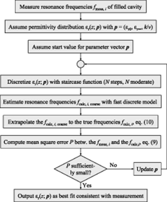
Figure 4. Algorithm to find the one permittivity distribution from the class of functions following from a first-order reaction which best explains measured resonance frequencies. The adaptation of the algorithm to other function classes is obvious.
Download figure:
Standard image High-resolution image3.3. Analytical test of optimization algorithm
To validate the feasibility of our method, let us consider a tubular reactor of length L = 200 mm and radius a = 62.5 mm, in which the starting substances A and B are mixed and react to product C. Let the mixture of A and B have the effective relative permittivity r0 = 1.2 and C have the relative permittivity r∞ = 2.5. Losses are neglected. The reaction is described as being of first order. The quotient of reaction rate and velocity of flow is assumed to be k/v = 0.0231 mm–1. The conversion at the end of the reactor is to reach about 99%.
For the case discussed, the relative permittivity along the reactor axis is given by model 2 in table 1. Therefore, if we model the reactor as a cavity consisting of N homogeneous segments, the effective permittivity of the material in the jth segment is given by equation (8) with equation (5).
Forward calculation yields the resonance frequencies listed in table 2 for N = 1000 and N = 200. The last row lists the result c of fitting the resonance frequencies computed with N = 50, 60, 70, 80, and 90 by equation (10). The frequency calculation by fitting is twice as fast as the computation of the resonance frequency with N = 200.
Table 2. Some TE11x mode resonance frequencies, calculated by different parameters/methods; cf. section 3.3 for geometry. The chosen modes are the lowest-order TE11x modes that are not evanescent in any segment of the discretized models.
| Computation method | Mode resonance frequency/GHz | |||
|---|---|---|---|---|
| TE112 | TE113 | TE114 | TE115 | |
| Segmented model, N = 1000 | 1.368154 | 1.774906 | 2.221292 | 2.688092 |
| ∼, N = 200 | 1.368124 | 1.774910 | 2.221298 | 2.688099 |
| Fit, equation (10) | 1.368120 | 1.774901 | 2.221308 | 2.688077 |
Let us assume that the resonance frequencies calculated with N = 1000 (five segments per mm) are accurate. It then follows that the associated material parameter distribution must be reconstructed by the inversion algorithm if the algorithm is passed the resonance frequencies. This is indeed the case. figure 5 shows the results when the inversion is based on a discretized cavity model with only N = 100 segments (2 mm length each) and (bad!) start values of k/v = 0.1 mm−1, r0 = 0.5, and r∞ = 1.6. The optimization algorithm, implemented in Matlab, finished in 120 s on a standard desktop PC (Xeon E31220 @ 3.1 GHz). It is expected that a compiled optimized C-code executable would converge much faster.
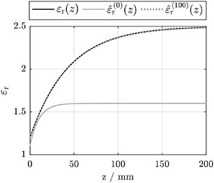
Figure 5. Results of analytical test (first-order reaction; see text). The black solid line is the true permittivity distribution r(z), the grey solid line is the estimated permittivity distribution r(0)(z) based on the bad start values passed to the reconstruction algorithm, and the dotted line is the estimated permittivity distribution r(100)(z) based on the output values of the reconstruction algorithm after the 100th iteration.
Download figure:
Standard image High-resolution image4. Experimental validation
4.1. Numerical experiments
The inversion algorithm was validated with synthetic measurement data. The input data to the algorithm were created by assuming one of the permittivity distributions 1–3 from table 1 inside a tubular reactor of given geometry and calculating the resonance frequencies either analytically (section 1, N = 1000) or numerically by the commercial FEA software HFSS (about 275000 elements). Four calculated resonance frequencies (synthetic measurement results) were passed to the inversion algorithm to check how well it reconstructs the underlying permittivity distribution. (The procedure is described by figure 4 with the first step replaced by a calculation of the resonance frequencies of the filled cavity.)
All permittivity distributions used the same parameters: a mixture of starting materials (r0 = 70) is converted to a product (r∞ = 80). The rate-determining term was set to k/v = 0.1 m−1.
In all cases, the convergence criterion from figure 4 was set to P < 1. If the algorithm had not converged after 100 iterations, it was aborted.
4.1.1. Zeroth-order reaction.
The result of the first numerical experiment, with model 1 from table 1, is visualized in figure 6. It is obvious that the reconstructed permittivity distribution is but a rough approximation of the true distribution, no matter if the analytically or the numerically calculated resonance frequencies are passed to the reconstruction algorithm. The reason is that the resonance frequencies are quite insensitive to the smaller permittivities in the region z < 100 mm. Any distribution with r(z) = 80 for 100 mm < z < 200 mm leads to similar resonance frequencies. Therefore, the reconstruction algorithm converges to one of many almost equivalent local minima. To find the global optimum, a multi-start algorithm may be useful [13], but the overall conclusion is that a zeroth-order reaction is not easily monitored by the present method.
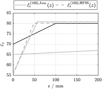
Figure 6. Permittivity distribution reconstructed using model 1 from table 1 (zeroth-order reaction). Black and grey solid lines as in figure 5.
Download figure:
Standard image High-resolution image4.1.2. First-order reaction.
The result of the second numerical experiment, with model 2 from table 1, is visualized in figure 7. In contrast to the zeroth-order reaction, the permittivity distribution caused by a first-order reaction is reconstructed exceedingly well.
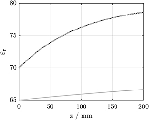
Figure 7. Permittivity distribution reconstructed using model 2 from table 1 (first-order reaction). Line types as in figure 6.
Download figure:
Standard image High-resolution image4.1.3. Second-order reaction.
The result of the third numerical experiment, with model 3 from table 1, is visualized in figure 8. The permittivity distribution caused by a second order reaction is reconstructed quite well, far better than model distribution 1 from table 1, but worse than model distribution 2 from table 1. As the reconstruction result based on analytically calculated resonance frequencies differs from the result based on numerically calculated resonance frequencies, the algorithm probably converged to different local optima in the two cases. Model function 2 may be suspected to be sensitive to input parameter errors.

Figure 8. Permittivity distribution reconstructed using model 3 from table 1 (second-order reaction). Line types as in figure 6.
Download figure:
Standard image High-resolution imageSome quantitative results of the numerical experiments from sections 4.1.1 through 4.1.3—the identified parameter values r0, r∞, and k/v—are listed in table 3 for comparison's sake.
One notes that all models had problems with the identification of the parameter k/v. The other two parameters presented fewer problems, and especially r∞ was reproduced by all models with small error.
Table 3. Results of the permittivity distribution reconstruction based on four resonance frequencies of the loaded cavity calculated either analytically or numerically by HFSS. The target (true) values of the distribution parameters were k/v = 0.1 m−1, r0 = 70, and r∞ = 80. E denotes the relative error of the reconstructed parameter value with respect to the target value.
| Origin of res. freq. | k/v 1000 m | r0 |
r∞
|
|||
|---|---|---|---|---|---|---|
| Value | E/% | Value | E/% | Value | E/% | |
| True r(z) as by model no. 1 from table 1 |
||||||
| Analytical | 17.6 | 76.0 | 56.1 | −19.9 | 80.8 | 1.0 |
| HFSS | 20.5 | 105.0 | 55.3 | −21.0 | 80.2 | 0.3 |
| True r(z) as by model no. 2 from table 1 |
||||||
| Analytical | 10.0 | 0.0 | 70.0 | 0.0 | 80.0 | 0.0 |
| HFSS | 9.3 | −7.0 | 70.1 | 0.1 | 80.3 | 0.4 |
| True r(z) as by model no. 3 from table 1 |
||||||
| Analytical | 22.0 | 120.0 | 71.1 | 1.6 | 76.6 | −4.3 |
| HFSS | 5.3 | −47.0 | 69.8 | −0.3 | 84.6 | 5.8 |
Model 1 produced high errors, except for the variable r∞. Model 2 resulted in relative errors below 1% in most cases, one exception being the result based on numerically calculated resonance frequencies. It is obvious that the proposed measurement method works extremely well for this model function. The quantitative results of model 3 confirm the previously made statement: model 3 works better than model 1, but worse than model 2.
4.1.4. Sigmoidal function as reaction-front model.
Yet another numerical experiment was conducted with the distribution function model no. 4 in table 1. It is treated separately as it has an additional parameter and is not based on a reaction order. Such a sigmoidal function approximates situations occurring with reaction fronts running through a catalyst. Consider, for example, the hypothetical monitoring of oxygen storage in a cerium oxide catalyst. The respective permittivities of the oxygen-less Ce2O3 and the oxygen-loaded CeO2 were chosen as r0 = 2.0 and r∞ = 1.4 based on [14, 23]. With the position a = 175 mm of the oxygen storage front and the slope parameter d = 10 mm, all parameters of the model function 4 are defined.
The result of this numerical experiment with model 4, based on five resonance frequencies, is visualized in figure 9. The permittivity distribution is reconstruted exceedingly well (cf. table 4).
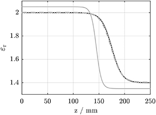
Figure 9. Permittivity distribution reconstructed using model 4 from table 1. Line types as in figure 6.
Download figure:
Standard image High-resolution imageTable 4. Results of the permittivity distribution reconstruction based on five resonance frequencies of the loaded cavity calculated either analytically or numerically by HFSS. The target (true) permittivity distribution was that of model no. 4 in table 1 with parameter values r0 = 2.0, r∞ = 1.4, a = 175 mm, and d = 10 mm. E denotes the relative error of the reconstructed parameter value with respect to the target value.
| Origin of res. freq. | a mm−1 | r0 |
r∞ |
d mm−1 | ||||
|---|---|---|---|---|---|---|---|---|
| Val. | E/% | Val. | E/% | Val. | E/% | Val. | E/% | |
| Analytical | 175 | 0 | 1.4 | 0 | 2.0 | 0 | 9.9 | 1 |
| HFSS | 174 | −0.6 | 1.4 | 0 | 2.0 | 0 | 10.3 | 3 |
4.2. Experiments with sand-filled cavity
A cylindrical cavity with length L = 380 mm and radius a = 62.5 mm was partially filled with sand (cf. figure 10). The target relative fill levels were 25%, 50%, 75%, and 100%, checked with a ruler. The boundary between the sand-filled region and the air-filled region was flat up to small bumps in the sand from the pouring-in process. The sand was dry and not compressed. The cavity was coupled with a small stub (LC = 5 mm, aC = 0.5 mm) at z = L/4, pointing in the radial direction.

Figure 10. Schematic drawing of the sand-filled cavity used for experiments.
Download figure:
Standard image High-resolution imageThe differences between the calculated and the measured resonance frequencies amounted to a few MHz, which was much larger than in the previous numerical experiments. As a consequence, the residuum of equation (9) was larger, too.
The start values for the parameter estimation were chosen close to the expected final values. In a real-time process monitoring scenario, the known result of a preceding measurement would provide these start values. The reconstructed permittivity distributions inside the cavity are shown in figure 11 for all investigated fill levels. The corresponding identified permittivities of sand and air are listed in table 5. The unphysical values for the relative permittivity of air (less than unity) have not been corrected to provide an indication of the magnitude of the measurement error.
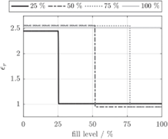
Figure 11. Permittivity distributions inside a sand-filled cavity reconstructed from measured cavity resonance frequencies.
Download figure:
Standard image High-resolution imageTable 5. Permittivities of sand and air experimentally determined with the sand-filled cavity experiment.
| Relative sand-fill level/% | Reconstructed parameters | |
|---|---|---|
| r, sand |
r, air |
|
| 25 | 2.45 | 1.01 |
| 50 | 2.56 | 0.95 |
| 75 | 2.55 | 0.95 |
| 100 | 2.52 | — |
| Ref. [23] | 2.55 | 1.00 |
4.3. Error analysis
It is of paramount importance to pass the unloaded resonance frequencies to the inversion algorithm. When loaded resonance frequencies are measured and compared with calculated unloaded frequencies, a perfect agreement between measurement and simulation can only be achieved by assuming 'wrong' material parameters in the simulation.
The error in the identified material parameters depends on many factors, e.g. the model function, its discretization, the number and types of observed resonance modes, the cavity geometry, etc. In an effort to shed more light on this issue, we repeated the analytical test from section 3.3 in a modified form. The synthetic measured resonance frequencies passed to the reconstruction algorithm for validation purposes were calculated with a discretization of N = 100 segments. The same discretization was used by the algorithm. Hence, in the absence of errors, the algorithm reproduces the exact material parameter distribution because it can reproduce the 'measured' resonance frequencies.
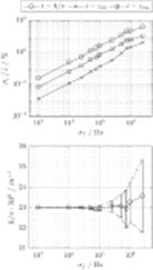
To emulate measurement errors, the resonance frequencies passed to the reconstruction algorithm were disturbed by additive white Gaussian noise (AWGN). For a given standard deviation σf of the noise, the reconstruction process was repeated 100 times. Figure 12(a) shows the standard deviations of the three distribution parameters r0, r∞, and k/v of the first-order reaction model estimated by the reconstruction algorithm as functions of the noise parameter σf. figure 12b shows the complete measurement result for the parameter k/v by the Guide to the Expression of Uncertainty in Measurement (GUM) [24].
Figure 12. Influence of measurement noise in the resonance frequencies passed to the reconstruction algorithm, for the example of a first-order reaction (model no. 2 in table 1). (a) Standard deviation of the reconstructed model parameters r0, r∞, and k/v, normalized to their respective mean values, as functions of the standard deviation σf of the AWGN corrupting the resonance frequencies. (b) Mean value and uncertainty interval at the 95-% level for the reconstructed parameter k/v.
Download figure:
Standard image High-resolution image
From these results, it is obvious that noise in the order of a few 100 kHz in the measured resonance frequencies (which are in the GHz range) has a negligible influence on the output parameter. Larger errors up to a standard deviation of 1 MHz lead to appreciable uncertainties in the identified material parameters, but may still be tolerable. A coarse condition monitoring is much better than no information.
5. Conclusion
We have investigated the problem of the reconstruction of axially inhomogeneous permittivity distributions in tubular reactors from measured cavity resonance frequencies of the reactor. The results are sufficiently promising to make us believe that the cavity perturbation method is suited in principle for the in-situ monitoring of chemical reactions or similar processes. The analytical, numerical, and experimental findings all indicate that the resulting error in an identified permittivity is in the order of 5%.
A frequency measurement noise below 10−4 (100 kHz for a 1 GHz resonance) was shown to have a negligible effect. In contrast, systematic errors due to the detuning of the cavity by the coupling are detrimental; the reconstruction algorithm must be passed unloaded resonance frequencies, not loaded ones.
In real-time monitoring situations, one can only measure a few resonance frequencies for reasons of time and effort. It will then be impossible to uniquely reconstruct an arbitrary material parameter distribution inside the cavity. As we have shown, the inclusion of a-priori knowledge about the process occurring inside the cavity enables one to both speed up the reconstruction and to tackle the ambiguity of the inverse problem. The assumption of a parametrized model function for the permittivity distribution in the cavity led to well-behaved and quickly solvable inversion problems requiring but a few resonance frequencies. However, as it turned out, some model functions are more sensitive to the material parameter distribution than others. The reconstruction of the distribution based on less sensitive model functions obviously does not work well.
As to the start values for the iterative reconstruction algorithm, the best choices in a continuous monitoring situation are the results of the previous measurement (parameter identification). This improves the convergence behavior very much.
Acknowledgments
This work was funded by the Deutsche Forschungsgemeinschaft (DFG, German Research Foundation)—Grant No. 389867475.