Automated Discovery of Local Rules for Desired Collective-Level Behavior Through Reinforcement Learning
 Tiago Costa
 Andres Laan
 Francisco J. H. Heras
 Gonzalo G. de Polavieja
- Collective Behavior Laboratory, Champalimaud Research, Lisbon, Portugal
Complex global behavior patterns can emerge from very simple local interactions between many agents. However, no local interaction rules have been identified that generate some patterns observed in nature, for example the rotating balls, rotating tornadoes and the full-core rotating mills observed in fish collectives. Here we show that locally interacting agents modeled with a minimal cognitive system can produce these collective patterns. We obtained this result by using recent advances in reinforcement learning to systematically solve the inverse modeling problem: given an observed collective behavior, we automatically find a policy generating it. Our agents are modeled as processing the information from neighbor agents to choose actions with a neural network and move in an environment of simulated physics. Even though every agent is equipped with its own neural network, all agents have the same network architecture and parameter values, ensuring in this way that a single policy is responsible for the emergence of a given pattern. We find the final policies by tuning the neural network weights until the produced collective behavior approaches the desired one. By using modular neural networks with modules using a small number of inputs and outputs, we built an interpretable model of collective motion. This enabled us to analyse the policies obtained. We found a similar general structure for the four different collective patterns, not dissimilar to the one we have previously inferred from experimental zebrafish trajectories; but we also found consistent differences between policies generating the different collective pattern, for example repulsion in the vertical direction for the more three-dimensional structures of the sphere and tornado. Our results illustrate how new advances in artificial intelligence, and specifically in reinforcement learning, allow new approaches to analysis and modeling of collective behavior.
1. Introduction
Complex collective phenomena can emerge from simple local interactions of agents who lack the ability to understand or directly control the collective [1–14]. Examples include cellular automata for pattern generation [3, 6, 10], self-propelled particles (SPP) [2, 4, 5, 7, 11, 13], and ant colony models for collective foraging and optimization [8, 12].
If in one of such systems we observe a particular collective configuration, how can we infer the local rules that produced it? Researchers have relied on the heuristic known as the modeling cycle [15, 16]. The researcher first proposes a set of candidate local rules based on some knowledge of the sensory and motor capabilities of the agents. The rules are then numerically simulated and the results compared with the desired outcome. This cycle is repeated, subsequently changing the rules until an adequate match between simulated trajectories and the target collective configuration is found.
Studies in collective behavior might benefit from a more systematic method to find local rules based on known global behavior. Previous work has considered several approaches. Several authors have started with simple parametric rules of local interactions and then tuned the parameters of the interaction rules via evolutionary algorithms based on task-specific cost functions [17, 18]. When the state space for the agents is small, a more general approach is to consider tabular rules, which specify a motor command for every possible sensory state [19].
These approaches have limitations. Using simple parametric rules based on a few basis functions produces models with limited expressibility. Tabular mapping has limited generalization ability. As an alternative not suffering from these problems, neural networks have been used as the function approximator [20–22]. Specifically, neural network based Q-learning has been used to study flocking strategies [23] and optimal group swimming strategies in turbulent plumes [24]. Q-learning can however run into optimization problems when the number of agents is large [25]. Learning is slow if we use Q-functions of collective states (e.g., the location and orientation of all agents) and actions, because the dimensionality scales with the number of agents. When implementing a separate Q-function for the state and action of each agent, the learning problem faced by each agent is no longer stationary because other agents are also learning and changing their policies simultaneously [26]. This violates the assumptions of Q-learning and can lead to oscillations or sub-optimal group level solutions [27].
Despite these difficulties, very recent work using inverse reinforcement learning techniques has been applied to find interaction rules in collectives [28, 29]. These approaches approximate the internal reward function each agent is following, and require experimental trajectories for all individuals in the collective. Here, we follow a different approach in which we aim at finding a single policy for all the agents in the collective, and with the only requirement of producing a desired collective configuration.
Our approach includes the following technical ingredients. We encode the local rule as a sensorimotor transformation, mathematically expressed as a parametric policy, which maps the agent's local state into a probability distribution over an agent's actions. As we are looking for a single policy, all agents have the same parametric policy, with the same parameter values, identically updated to maximize a group level objective function (total reward during a simulated episode) representing the desired collective configuration. A configuration of high reward was searched for directly, without calculating a group-level value function and thus circumventing the problem of an exploding action space. For this search, we use a simple algorithm of the class of Evolution Strategies (ES), which are biologically-inspired algorithms for black-box optimization [30, 31]. We could have chosen other black-box optimization algorithms instead, such as particle swarm algorithms [32]. However, this ES algorithm has recently been successful when solving Multi-Agent RL problems [33], and when training neural-network policies for hard RL problems [34].
We applied this approach to find local rules for various experimentally observed schooling patterns in fish. Examples include the rotating ball, the rotating tornado [35], the full-core rotating mill [36], and the hollow-core mill [37]. To our knowledge, with the exception of the hollow-core mill [38, 39], these configurations have not yet been successfully modeled using SPP models [11].
2. Methods
We placed the problem of obtaining local rules of motion (policies) that generate the desired collective patterns in the reinforcement learning framework [40]. As usual in reinforcement learning, agents learn by maximizing a reward signal obtained from their interaction with the environment in a closed-loop manner, i.e., the learning agents's actions influence its later inputs Figure 1. To describe this interaction, it is necessary to specify a model of the agents and the environment, a reward function, a policy representation and a method to find the gradient of the reward function with respect to the parameters of the policy. Both the environment update and the reward are history-independent, and thus can be described in the framework of multi-agent Markov decision processes [41]. We describe the four components (agent and environment model, reward function, policy parameterization, and learning algorithm) in the following subsections.
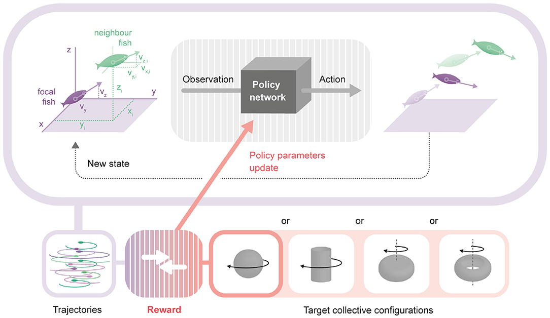
Figure 1. Framework to obtain an interaction model producing a desired collective behavior. Upper: The policy network is a neural network that transforms the observation of an agent into its action. Its parameters are the same for all agents and chosen to produce a target collective behavior. For each focal fish (purple), the observation used to generate actions is formed by: the horizontal and vertical components of the focal fish, plus the three components of the relative position and three components of the absolute velocity of each of the neighbors. In the diagram, a single example neighbor fish is shown (green). From the observations of each focal fish, the policy network generates an action for each fish, modifying their heading and speed in the next time step according to the physics imposed for the environment. The new locations, velocities and orientations define a new state. Lower: Repeating the loop described above a number of times, we obtain a trajectory for each fish. We compare the trajectories with the selected desired configuration (rotating sphere, rotating tornado, rotating hollow-core mill and rotating full-core mill) producing a reward signal that it is used to change the parameters of the policy network.
2.1. A Model of the Agent and the Environment
We model fish as point particles moving trough a viscous three-dimensional environment. In this section, we explain how we update the state of each and every fish agent.
Let us define a global reference frame, with Z axis parallel to the vertical, and X and Y in a horizontal plane. Length is expressed in an arbitrary unit, which we call body length (BL) because it corresponds to the body length of agents in the retina experiments that we describe in the Supplementary Text.
In this reference frame, we consider a fish agent moving with a certain velocity. We describe this velocity as three numbers: the speed V, elevation angle θ (i.e., its inclination angle is ) and azimuth angle ϕ. In the next time step, we update the X, Y, and Z coordinates of the fish as
where δ corresponds to the duration of a time step (see Table 1 and Table S2 for parameter values).
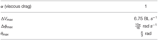
Table 1. Environment parameters described in the methods.
The elevation angle, azimuth angle change, and speed change are updated based on three outputs of the policy network, p1, p2, and p3, each bounded between 0 and 1. The three outputs of the policy network are independently sampled at time t from a distribution determined by the observation at time step t (see section 2.3).
The azimuth, ϕ, is updated using the first output of the policy, p1:
with Δϕmax the maximum change in orientation per unit time, and δ is the time step duration.
The elevation angle, θ, is calculated based on the second output of the policy network, p2, as
where the maximum elevation is θmax
Finally, the speed change is the sum of two components: a linear viscous drag component (with parameter α) and an active propulsive thrust determined by the third output of the policy network, p3,
The parameter ΔVmax is the maximum active change of speed of a fish. This equation for the change in velocity captures that deceleration in fish is achieved through the passive action of viscous forces [42].
At the beginning of each simulation, we initialize the positions and velocities of all fish randomly (see Supplementary Text for details). The same state update Equations (1)–(6) are applied identically to all fish while taking into account that each one has a different position, speed, orientation and neighbors.
2.2. Reward Function
In our simulations, the final behavior to which the group converges is determined by the reward function. We aim to model four different collective behaviors, all of which have been observed in nature. These behaviors are called the rotating ball [16], the rotating tornado [35], the rotating hollow core mill [11, 37], and the rotating full core mill [36].
At each time step, the configuration of agents allows to compute an instantaneous group level reward r(t). The objective of the reinforcement learning algorithm is to find ways to maximize the reward R in the episode, which is the sum of r(t) over the N steps of simulation time. The instantaneous reward r(t) is composed of several additive terms. In this section we will explain the terms used in the instantaneous reward function for the rotating ball, and in Supplementary Text we give mathematical expressions for the terms corresponding to the four collective structures.
The first term is composed of collision avoidance rewards, rc. It provides an additive negative reward for every pair of fish (i, j) based on their mutual distance di,j. Specifically, for each neighbor we use a step function that is zero if di,j > Dc and −1 otherwise. This term is meant to discourage the fish from moving too close to one another.
The second term is an attraction reward, ra, which is negative and proportional to the sum of the cubed distances of all fish from the center of mass of the group. This attraction reward will motivate the fish to stay as close to the center of mass as possible while avoiding mutual collisions due to the influence of the collision reward. Together with rc, it promotes the emergence of a dense fish ball.
The third term in the instantaneous reward, rr, is added to promote rotation. We calculate for each fish i its instantaneous angular rotation about the center of mass in the X − Y plane, Ωi. The rotation term, rr, is the sum of beta distributions of that angular rotation across all fish.
The fourth and final term, rv, penalizes slow configurations. It is a step function that is 0 if the mean speed is above Vmin and −1 otherwise. Vmin is small enough to have a negligible effect in the trained configuration, but large enough to prevent the agents from not moving. As such, this last term encourages the agents to explore the state-action space by preventing them from remaining still.
The reward functions designed to encourage the emergence of a rotating tornado and the rotating mills are described in the Supplementary Text but they in general consist of similar terms.
Unlike previous work in which each agent is trying to maximize an internal reward function [28, 29], we defined the reward functions globally. Although each agent is observing and taking actions independently, the collective behavior is achieved by rewarding the coordination of all the agents, and not their individual behaviors.
2.3. The Policy Network
We parameterize our policy as a modular neural network with sigmoid activation functions, Figure 2. In our simulations, all fish in the collective are equipped with an individual neural network. Each network receives the state observed by the corresponding agent and outputs an action that will update its own position and velocity.
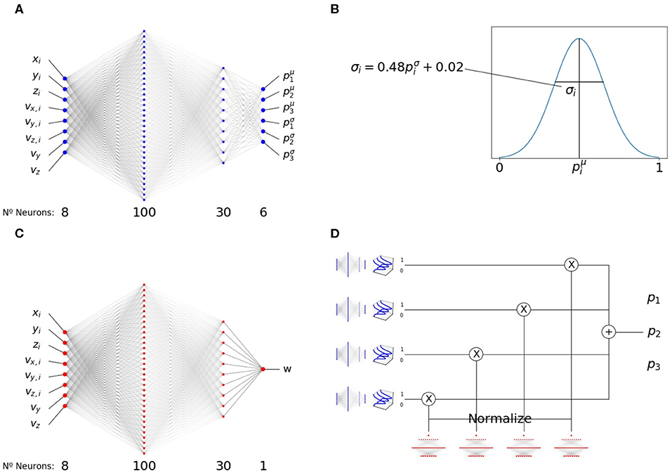
Figure 2. Modular structure of the policy network. (A) Pair-interaction module, receiving asocial variables, vy and vz, and social variables, xi, yi, zi, vx,i, vy,i, vz,i, from a single neighbor i, and outputting 6 numbers (three mean values and three variance values). (B) Three numbers are sampled from three clipped Gaussian distributions with mean and variances given by the output of the pair-interaction module. (C) Aggregation module. Same structure as A, but with a single output that is passed through an exponential function to make it positive. (D) Complete structure of the modular network, showing how the outputs of the pair-interaction and aggregation modules are integrated. The resulting output, p1, p2, p3, determines the heading and speed of the focal fish in the next time step.
All the networks have the same weight values, but variability in the individual behaviors is still assured for two reasons. First, we use stochastic policies, which makes sense biologically, because the same animal can react differently to the same stimulus. In addition, a stochastic policy enables a better exploration of the state-action space [43]. Second, different fish will still act following different stochastic distributions if they have different surroundings. In the next section we will describe these networks and the implementation of stochasticity in the policy.
2.3.1. Inputs and Outputs
At each time step, the input to the network is information about the agent surroundings. For each focal fish, at every time step we consider an instantaneous frame of reference centered on the focal fish, with the z axis parallel to the global Z axis, and with the y axis along the projection of the focal velocity in the X − Y plane. For each neighbor, the variables considered are xi, yi, zi (the components of the neighbor i position in the new frame of reference) and vx,i, vy,i, vz,i (the components of the neighbor velocity in the new frame of reference). In addition, we also use vy and vz (the components of the focal fish velocity in the new frame of reference). Please note that the frame is centered in the focal fish, but it does not move nor rotate with it, so all speeds are the same as in the global frame of reference.
The policy network outputs three numbers, p1, p2, and p3 (see next section for details), that are then used to update the agent's azimuth, elevation angle and speed, respectively.
2.3.2. Modular Structure
To enable interpretability, we chose a modular structure for the policy neural network. Similar to our previous work [44], we chose a network architecture with two modules, Figure 2. Both modules have the 8 inputs we detailed above and two hidden layers of 100 and 30 neurons.
The first module, the pairwise-interaction module, contains 6 output neurons, Figure 2A. For each neighbor i, they produce 6 outputs . The outputs are symmetrized with respect to reflections in the x − y and y − z planes, with the exception of p1,i (mean azimuth angle change, anti-symmetrized with respect to the x − y plane) and p2,i (mean elevation change, anti-symmetrized with respect to the y − z plane).
The previous values, , encode the mean and the scaled variance of three normal distributions (clipped between 0 and 1) used to sample three variables,
For each neighbor, i, we sample values of p1,i, p2,i and p3,i independently from the respective distributions, Figure 2B.
The second module, the aggregation module, has a single output, W (Figure 2C). It is symmetrized with respect to both the x − y and y − z planes. It is clipped between −15 and 15 and there is an exponential non-linearity after the single-neuron readout signal to make it positive.
The final output combines both modules, Figure 2D. It is calculated by summing the outputs of the pairwise-interaction modules applied to the set of all neighbors, , using the outputs of the aggregation module as normalized weights,
where we combined p1,i, p2,i, and p3,i as components of a vector Pi. The final outputs used to update the dynamics of the agent, p1, p2, p3 are the components of P.
Everywhere in this paper, the set of neighbors considered, , consists of all the other fish in the same environment as the focal. Even if this is the case, note that the introduction of the aggregation module acts as a simulated attention that selects which neighbors are more relevant for a given state and policy.
2.4. Optimizing the Neural Network Parameters
Following previous work [33, 34], we improved the local rule using an “Evolution Strategies” algorithm [30, 31]. The text in this section is an explanation of its main elements.
Let us denote by the neural network weights at every iteration of the algorithm, and by the reward obtained in that iteration (sum during the episode). A change in parameters that improves the reward can be obtained by following the gradient with small steps (gradient ascent),
where λ is the learning rate (see Supplementary Text for the values of hyper-parameters in our simulations). Repeating this gradient ascent on the reward function, we approach the desired collective behavior over time. As we explain below, we perform this gradient while co-varying the parameters of all agents. In contrast, the naive application of policy gradient would be equivalent to performing the gradient with respect to the parameters of one of the agents, keeping the parameters of others constant. This could produce learning inefficiencies or even failure to find the desired policy.
We estimate the gradient numerically from the rewards of many simulations using policy networks with slightly different parameters. We first sample K vectors independently from a spherical normal distribution of mean 0 and standard deviation σ, with as many dimensions as parameters in the model. We define . We calculate 2K parameter vectors . We then conduct a single simulation of a fish collective —all agents in the same environment sharing the same values and we record the reward Ri. Then, we use as an approximation of to perform gradient ascent [34].
We refer to Figure 3 for four example training runs using the algorithm, and to Figure 4 for the pseudo-code of the algorithm.
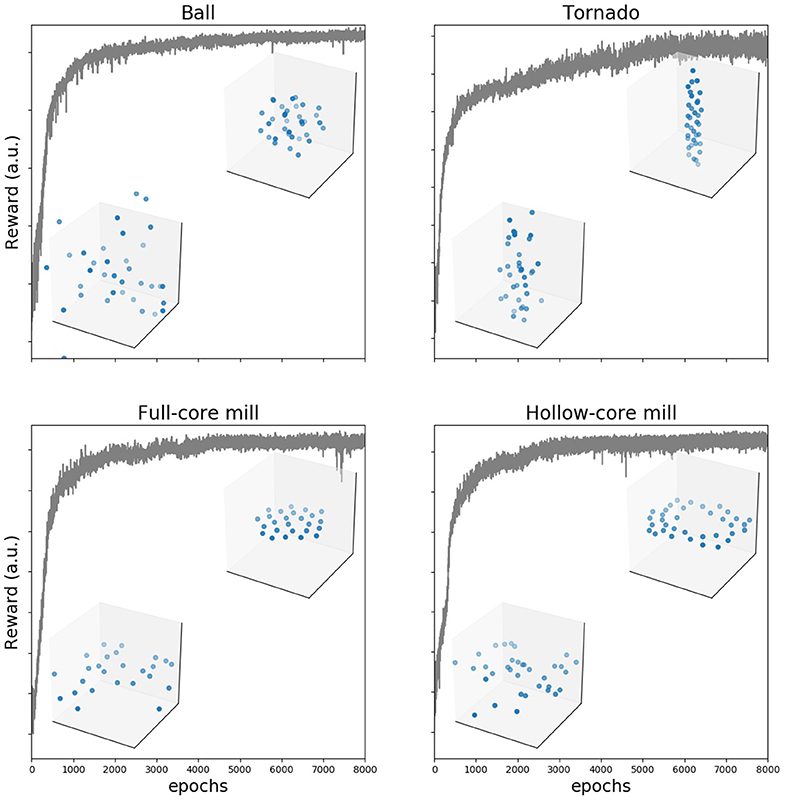
Figure 3. Training makes reward to increase and group behavior to converge to the desired configuration. Reward as a function of number of training epochs in an example training cycle for each of the four configurations. In each of the examples, we show two frames (agents shown as blue dots) from the generated trajectories, one early in the training process (100 epochs) and a second after the reward plateaus (8,000 epochs).
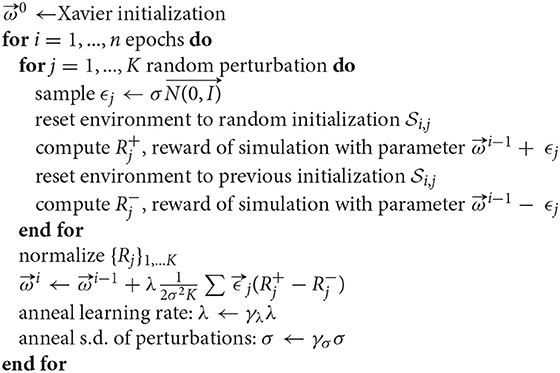
Figure 4. Evolution strategies algorithm.
2.5. Measurements of XY-Plane Interaction
As in previous work [44], we described changes in the azimuth angle using the approximate concepts of attraction, repulsion, and alignment. We define the attraction-repulsion and the alignment score as useful quantifications of these approximate concepts. Please note that these scores are not related to reward.
We obtained the attraction-repulsion and alignment scores from a centered and scaled version of :
where we chose to only explicitly highlight its dependence with the relative neighbor orientation in the XY plane, ϕi. This relative neighbor orientation can be calculated as the difference of the azimuth angle of the neighbor and the azimuth angle of the focal fish.
Attraction-repulsion score is defined by averaging over all possible relative orientations of the neighbor in the XY plane.
We would say there is attraction (repulsion) when the score is positive (negative).
The alignment score is defined as
As in [44], we arbitrarily decided that alignment is dominant (and thus that the point is in the alignment area) if changes sign when changing the relative orientation of the neighbor in the XY plane, ϕi. Otherwise, it is in an attraction or repulsion area, depending on the sign of the attraction-repulsion score [44]. Under this definition, repulsion (attraction) areas are the set of possible relative positions of the neighbor which would make a focal fish turn away (toward) the neighbor, independently of the neighbor orientation relative to the focal fish
3. Results
To simulate collective swimming, we equipped all fish with an identical neural network. At each time step, the neural network analyzes the surroundings of each fish and produces an action for that fish, dictating change in its speed and turning, Figure 1. Under such conditions, the neural network encodes a local rule and by varying the weights within the network, we can modify the nature of the local rule and thus the resulting group level dynamics.
As in previous work [44], we enabled interpretability by using a neural network built from two modules with a few inputs and few outputs each, Figure 2. A pairwise-interaction module outputs turning and change of speed with information from a single neighbor, i, at a time. It is composed of two parts. The first part outputs in a deterministic way mean values and variances for each of the three parameters encoding turning and change of speed, Figure 2A. The second part consists in sampling each parameter, p1,i, p2,i, p3,i, from a clipped Gaussian distribution with the mean and variance given by the outputs of the first part, Figure 2B.
An aggregation module outputs a single positive number expressing the importance carried by the signal of each neighbor, Figure 2C. The final outputs of the complete modular neural network are obtained by summing the results of the pairwise-interaction module, weighting them by the normalized outputs of the aggregation module, Figure 2D. The final outputs, p1, p2 and p3, determine the motor command. We perform these computations for each agent, and use the outputs to determine the position and speed of each agent in the next time step (Equations 1–3).
We introduced a reward function, measuring how similar are the produced trajectories to the desired group behavior (see section 2 for details). We used one of four different reward functions to encourage the emergence of one of four different collective configurations, all of which have been observed in natural groups of fish. These patterns are the rotating ball, the rotating tornado, the rotating hollow core mill and the rotating full core mill.
We used evolutionary strategies to gradually improve the performance of the neural network at the task of generating the desired collective configurations. The value of the reward function increased gradually during training for all four patterns, Figure 3. After several thousand time steps, the reward plateaued and the group collective motion was visually highly similar to the desired one (see Supplementary Videos 1–4). We tested that the agents learned to generate the desired collective configurations by using independent quantitative quality indexes (Supplementary Text and Figure S1). They show that agents learn first to come together into a compact formation, and then to move in the right way, eventually producing the desired configurations. We also checked that the configurations are formed also when the number of agents is different to the number used in training (see Supplementary Videos 5–8 for twice as many agents as those used in training).
3.1. Description of Rotating Ball Policy
Here, we use the low dimensionality of each module in terms of inputs and outputs to describe the policy with meaningful plots. We describe here the policy of the rotating ball (Figure 5). The equivalent plots for the other three configurations can be found in Figures S2–S4.
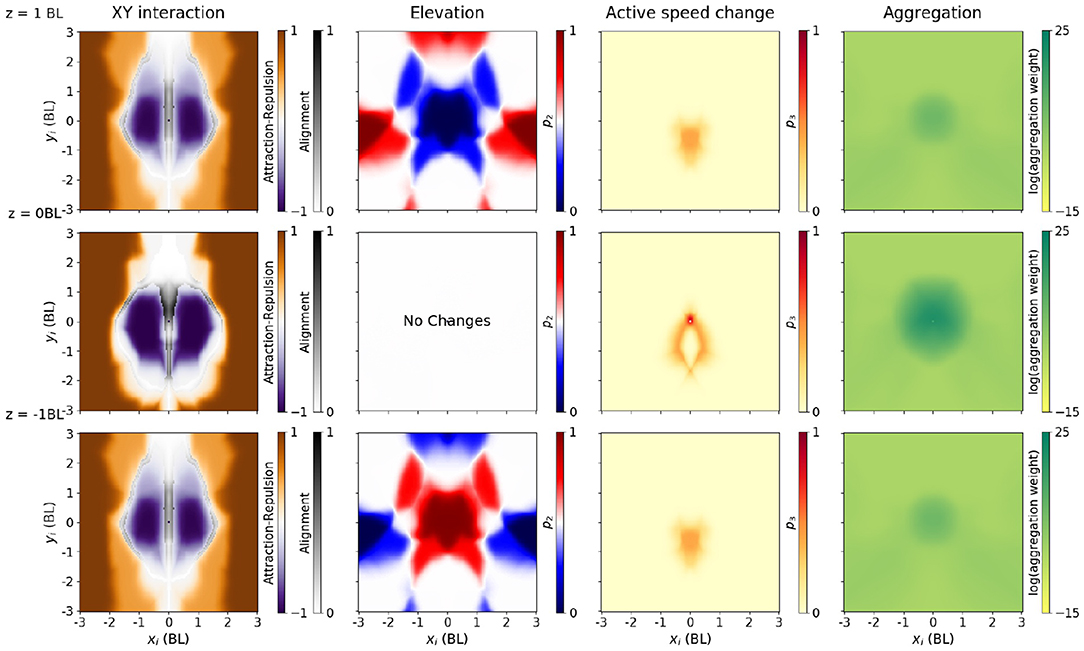
Figure 5. Policy producing a rotating ball, as a function of neighbor relative location. Each output (three from the pair-interaction, one from the aggregation) is shown in a different column. All columns have three diagrams, with the neighbor 1 BL above (top row), in the same XY plane (middle row) and 1 BL below the focal (bottom row). Speed of both the focal and neighbor has been fixed to the median in each configuration. In addition, in columns 2–4, we plot the average with respect to an uniform distribution over all possible relative neighbor orientations (from −π to π). First column: Interaction in the XY plane (change of azimuth). Instead of plotting p1, we explain interaction using the approximate notions of alignment (gray), attraction (orange), and repulsion (purple) areas, as in [44]. Alignment score (gray) measures how much the azimuth changes when changing the neighbor orientation angle, and it is computed only in the orientation areas (see Methods, Section 2.5). Attraction (orange) and repulsion scores (purple) measure how much the azimuth change when averaging across all relative orientation angles, and we plot it only outside orientation areas. Second column: Elevation angle, through the mean value of the p2 parameter. Blue areas indicate that the focal fish will move downwards (p2 < 0.5), while red areas indicate that the focal fish will move upwards (p2 > 0.5). Third column: Active change in speed, through the mean value of the p3 parameter. Darker areas (large mean p3) indicate increase in speed, and lighter areas indicate passive coast. Fourth column: Output of the aggregation module. Neighbors in the darker areas weight more in the aggregation.
The pairwise-interaction module outputs three parameters for each focal fish, all bounded between 0 and 1. The first one, p1, determines the change in azimuth, that is, rotations in the XY plane (Figure 5, first column). To further reduce dimensionality in the plots, we simplify the description of the policy in this XY plane by computing attraction-repulsion and orientation scores (see Equations 12, 13, section 2). These scores quantify the approximate concepts of attraction, repulsion and orientation. In Figure 5, we plot the alignment score in the areas where alignment is dominant, and the attraction-repulsion score otherwise.
The attraction areas give the neighbor positions in this XY plane which make a focal fish (located at xi = yi = 0) swim toward the neighbor, independently of the neighbor orientation (Figure 5, first column, orange). The focal fish turns toward the neighbor if the neighbor is far (> 1.5 BL). Repulsion areas are the relative positions of the neighbor which make a focal fish swim away from the neighbor (Figure 5, first column, purple). If the neighbor is closer than 1 BL, but not immediately in front or at the back of the focal, the focal tends to turn away from the neighbor (purple). In the areas where alignment is dominant (alignment areas), we plotted the alignment score (Figure 5, first column, gray). If the neighbor is at an intermediate distance, or in front or in the back of the focal fish, the focal fish tends to orient with respect to the neighbor in the XY plane.
The second parameter, p2, determines the elevation angle (Figure 5, second column). p2 is 0.5 on average, and thus elevation angle is zero on average, when the neighbor is on the same XY plane as the focal (Figure 5, second column, second row). When the neighbor is above, the focal agent tends to choose a negative elevation when the neighbor is close (Figure 5, second column, blue), and a positive elevation if it is far (red). The opposite happens when the neighbor is below: the focal agent tends to choose a positive elevation when the neighbor is close, and a negative elevation if it is far (Figure 5, second column, third row).
The third parameter, p3, determines the active speed change (Figure 5, third column). The active speed change is small, except if the neighbor is in a localized area close and behind the focal.
The aggregation module outputs a single positive output, determining the weight of each neighbor in the final aggregation. In the rotating ball policy, the neighbors that are weighted the most in the aggregation are the ones closer than 1 BL from the focal (Figure 5, third column). Neighbors located in a wide area behind the focal, but not exactly behind it, are assigned a moderate weight.
Note that the aggregation module is not constrained to produce a local spatial integration, since the network has access to every neighboring fish. However, we can observe how an aggregation module like the one shown for the rotating ball (Figure 5, third column) would preferably select a subset of closest neighbors—i.e., integration is local in space. This is also true for the other configurations: for each desired collective configuration we could always find policies with local integration (e.g., Figures S2–S4).
3.2. Description of Policy Differences Between Configurations
In the previous section, we described the policy we found to best generate a rotating ball. The policies we found that generate the other three configurations have many similarities and some consistent differences, Figure 6. In this section, we will highlight these differences.
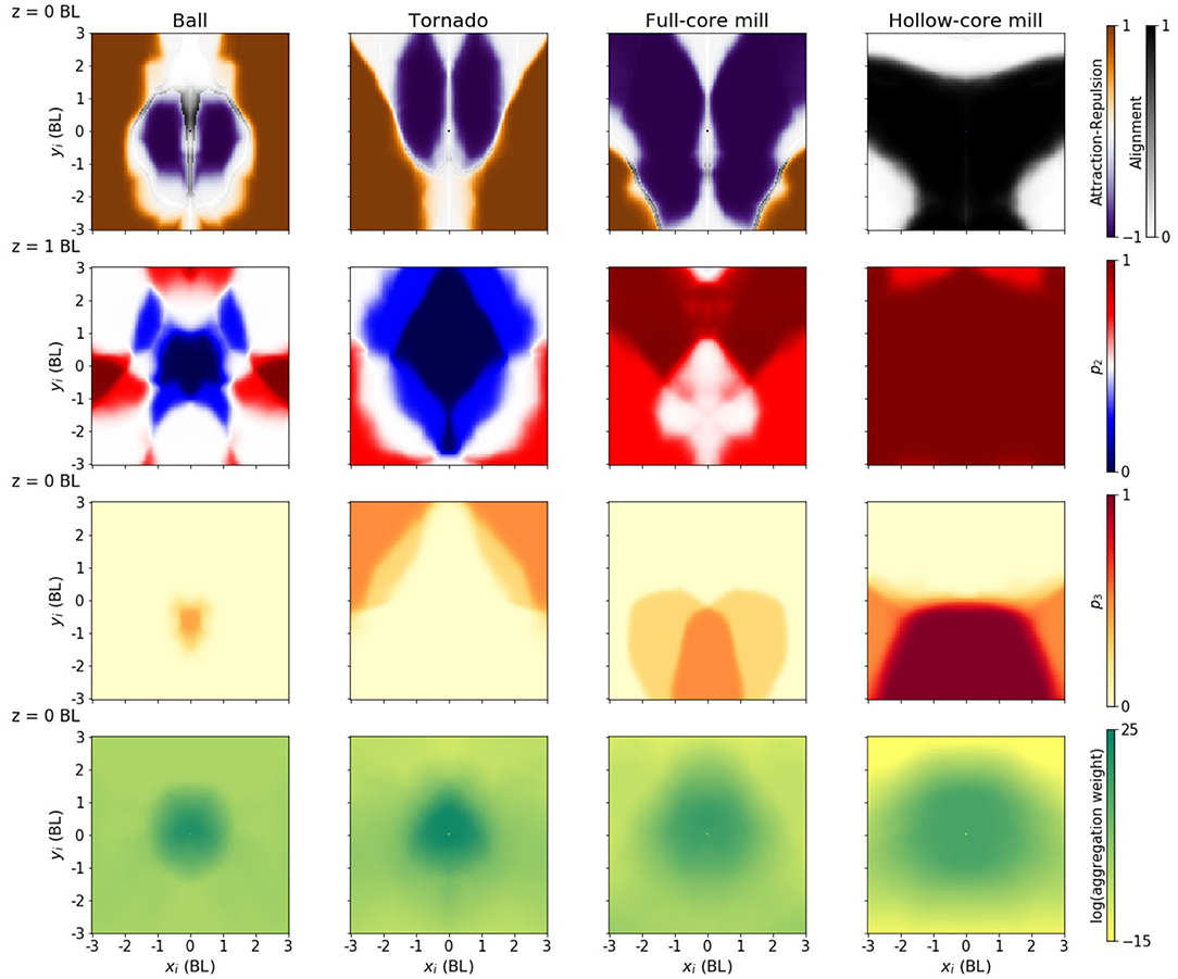
Figure 6. Policies producing different configurations. Each column corresponds to one of the four desired configurations. Each panel is the equivalent of the middle row in Figure 5, except in the case of the elevation (second column), that is equivalent to the panel in the top row. For each configuration, the speed of the focal and neighbor has been fixed to the configuration median: 0.42, 0.32, 0.75, and 1.54 BL/s, respectively.
The policy generating a tornado has an attraction-repulsion pattern somewhere in between the rotating ball and the full core milling (Figure 6, first row). The major feature that distinguishes this policy from the others is a strong repulsion along the z-axis, i.e., the area of the plot where the focal fish changes elevation to move away from the neighbor is larger (Figure 6, second column, second row, blue area). This was expected, as to form the tornado the agents need to spread along the z-axis much more than they do in the other configurations.
The policy generating a full-core mill has an increased repulsion area, particularly in the frontal and frontal-lateral areas (Figure 6, third column, first row, purple areas). The policy generating a hollow-core mill has an increased alignment area, weakening the repulsion area (Figure 6, fourth column, first row, gray area). It also has an increased area with a high change in velocity (Figure 6, fourth column, third row, red area). Both mill policies have an extended aggregation area, especially the hollow core (Figure 6, third and fourth column, fourth row), and lack an area where the focal fish changes elevation to move away from the neighbor (Figure 6, third and fourth column, second row, red area). The almost absence of repulsion in the z-direction makes both mills to be 2D structures, whereas repulsion in the sphere and tornado makes them 3D.
The highlighted differences between policies are robust (see Figure 5 and the Supplementary Material for Figures S2–S4 and Figures S6–S13 to see the robustness of the results in different runs). For instance, we have compared the policies by restricting the fish to move at the median speed is each configuration. The highlighted differences are still valid when the fish move with a common median speed across configurations (Figure S5).
3.3. Adding a Retina to the Agents
In the preceding section, the observations made by each agent were simple variables like position or velocities of neighbors. This simplification aided analysis, but animals do not receive external information in this way but by sensory organs.
We checked whether we could achieve the group configuration we have studied when the input to the policy for each agent is the activation of an artificial retina observing the other agents. The retina is modeled using a three-dimensional ray-tracing algorithm: from each agent, several equidistant rays project until they encounter a neighbor, or up to a maximum ray length r. The state, i.e., the input to the policy, is the list of the ray lengths. Information about the relative velocity was also given as input to the policy by repeating this computation with the current position and orientation of the focal, but the previous position of all the other agents. See Supplementary Text for a detailed description.
We approximated the policy using a single fully-connected network. Using the interaction and attention modules described in section 2.3.2 would not have added interpretability in this case, because the number of inputs is too large. By using the same evolutionary strategy, we were able to obtain a decision rule leading to the desired collective movement configurations (Supplementary Videos 9–12).
Although these configurations were qualitatively similar to the ones we obtained with the modular network (Figure S14), the average inter-agent distance was greater. This resulted in less compact configurations (Tables S3, S5). This effect might be the result of the increased complexity and decreased accuracy of the inputs given to the policy by the retina, which causes the agents to avoid each other more than in simulations without retina.
4. Discussion
We have applied evolutionary strategies (ES) to automatically find local rules able to generate desired group level movement patterns. Namely, we found local rules that generate four complex collective motion patterns commonly observed in nature [35, 45]. Three of these four patterns have, to our knowledge, not yet been generated using self-propelled particle models with local rules.
We used neural networks as approximators of the policy, the function mapping the local state to actions. The naive use of a neural network would produce a black-box model, that can be then analyzed with different post-hoc explainability strategies (inversion [46], saliency analysis [47], knowledge distillation [48], etc.; see [49, 50] for reviews). Instead, as we did in [44], we designed and trained a model that is inherently transparent (interpretable). This alternative improves our confidence in the model understandability: the model is its own exact explanation [51].
We used a modular policy network, composed by two modules. Each module is an artificial neural network with thousands of parameters, and therefore it is a flexible universal function approximator. However, we can still obtain insight, because each module implements a function with low number of inputs and outputs that we can plot [44]. Similar to what we obtained from experimental trajectories of zebrafish [44], we found the XY-interaction to be organized in areas of repulsion, orientation, and attraction, named in order of increasing distance from the focal fish. We were also able to describe differences between the policies generating each of the configurations.
To find the local rules generating the desired configurations, we used a systematic version of the collective behavior modeling cycle [15]. The traditional collective behavior modeling cycle begins with the researcher proposing a candidate rule and tuning it through a simulation based feedback process. Here, we parameterize the local rule as a neural network. Since neural networks are highly expressive function approximators which can capture a very diverse set of possible local rules, our method automates the initial process of finding a set of candidate rules. As in the case of the traditional modeling cycle, our method also relies on a cost function (the reward function) and numerical simulations to measure the quality of a proposed rule. The process of rule adaptation is automated by following a gradient of the reward function with respect to neural network weights. Just like the modeling cycle, our method uses iterations that gradually improve the policy until it converges to a satisfactory solution.
There are theoretical guarantees for convergence in tabular RL, or when linear approximators are used for the value functions [40]. However, these theoretical guarantees do not normally extend to the case where neural networks are used as function approximators [52], nor to multi-agent RL [25]. Here we report an application where the ES algorithm was able to optimize policies parameterized by deep neural networks in multi-agent environments. To our knowledge, there were no theoretical guarantees for convergence for our particular setting.
The method we have proposed could have several other interesting applications. In cases where it is possible to record rich individual level data sets of collective behavior, it can be possible to perform detailed comparisons between the rules discovered by our method and the ones observed in experiments [44, 53]. The method could also be applicable to answer more hypothetical questions such as what information must be available in order for a certain collective behavior to emerge. Animals may interact in a variety of ways including visual sensory networks [54], vocal communication [55], chemical communication [56] and environment modification (stigmergy) [57]. Animals also have a variety of cognitive abilities such as memory and varying sensory thresholds. By removing or incorporating such capabilities into the neural networks it is now possible to theoretically study the effects these factors have on collective behavior patterns.
Here we relied on an engineered reward function because the behaviors we were modeling have not yet been recorded in quantitative detail. In cases where trajectory data is available, detailed measures of similarity with observed trajectories can be used as a reward [33, 58]. Moreover, we can use adversarial classifiers to automatically learn these measures of similarity [19, 59]. Further interesting extensions could include creating diversity within the group by incorporating several different neural networks into the collective and studying the emergence of behavioral specialization and division of labor [60].
The present work may be used as a normative framework when the rewards used represent important biological functions. While prior work using analytic approaches has been successful for simple scenarios [42, 61], the present approach can extend them to situations in which no analytic solution can be obtained.
Data Availability Statement
The datasets were generated using the software from https://gitlab.com/polavieja_lab/rl_collective_behaviour.
Author Contributions
AL and GP devised the project. TC, AL, FH, and GP developed and verified analytical methods. TC wrote the software, made computations and plotted results with supervision from AL, FH, and GP. All authors discussed the results and contributed to the writing of the manuscript.
Funding
This work was supported by Fundação para a Ciência e a Tecnologia (www.fct.pt) PTDC/NEU-SCC/0948/2014 (to GP and contract to FH), Congento (congento.org) LISBOA-01-0145-FEDER-022170, NVIDIA (nvidia.com) (FH and GP), and Champalimaud Foundation (fchampalimaud.org) (GP). The funders had no role in study design, data collection and analysis, decision to publish, or preparation of the manuscript.
Conflict of Interest
The authors declare that the research was conducted in the absence of any commercial or financial relationships that could be construed as a potential conflict of interest.
Acknowledgments
We are grateful to Francisco Romero-Ferrero and Andreas Gerken for discussions.
Supplementary Material
The Supplementary Material for this article can be found online at: https://www.frontiersin.org/articles/10.3389/fphy.2020.00200/full#supplementary-material
Supplementary Video 1. Simulation of the agents trained to adopt a Rotating ball, with the modular deep networks. Here the number of agents is the same as the number of agents used in the training.
Supplementary Video 2. Simulation of the agents trained to adopt a Tornado, with the modular deep networks. Here the number of agents is the same as the number of agents used in the training.
Supplementary Video 3. Simulation of the agents trained to adopt a Full core milling, with the modular deep networks. Here the number of agents is the same as the number of agents used in the training.
Supplementary Video 4. Simulation of the agents trained to adopt a Hollow core milling, with the modular deep networks. Here the number of agents is the same as the number of agents used in the training.
Supplementary Video 5. Simulation of the agents trained to adopt a Rotating ball, with the modular deep networks. Here the number of agents is 70 while the number of agents used in training is 35.
Supplementary Video 6. Simulation of the agents trained to adopt a Tornado, with the modular deep networks. Here the number of agents is 70 while the number of agents used in training is 35.
Supplementary Video 7. Simulation of the agents trained to adopt a Full core milling, with the modular deep networks. Here the number of agents is 70 while the number of agents used in training is 25.
Supplementary Video 8. Simulation of the agents trained to adopt a Hollow core milling, with the modular deep networks. Here the number of agents is 70 while the number of agents used in training is 35.
Supplementary Video 9. Simulation of the agents trained to adopt a Rotating ball, when the network received the activation of a simulated retina as input.
Supplementary Video 10. Simulation of the agents trained to adopt a tornado, when the network received the activation of a simulated retina as input.
Supplementary Video 11. Simulation of the agents trained to adopt a full core milling, when the network received the activation of a simulated retina as input.
Supplementary Video 12. Simulation of the agents trained to adopt a hollow core milling, when the network received the activation of a simulated retina as input.
References
1. Smith A. An Inquiry into the Nature and Causes of the Wealth of Nations. Vol. 2. London: W. Strahan and T. Cadell (1776).
2. Aoki I. A simulation study on the schooling mechanism in fish. Bull Japan Soc Sci Fish. (1982) 48:1081–8. doi: 10.2331/suisan.48.1081
3. Wolfram S. Statistical mechanics of cellular automata. Rev Modern Phys. (1983) 55:601. doi: 10.1103/RevModPhys.55.601
4. Vicsek T, Czirók A, Ben-Jacob E, Cohen I, Shochet O. Novel type of phase transition in a system of self-driven particles. Phys Rev Lett. (1995) 75:1226. doi: 10.1103/PhysRevLett.75.1226
5. Helbing D, Molnar P. Social force model for pedestrian dynamics. Phys Rev E. (1995) 51:4282. doi: 10.1103/PhysRevE.51.4282
7. Levine H, Rappel WJ, Cohen I. Self-organization in systems of self-propelled particles. Phys Rev E. (2000) 63:017101. doi: 10.1103/PhysRevE.63.017101
8. Bonabeau E, Dorigo M, Theraulaz G. Inspiration for optimization from social insect behaviour. Nature. (2000) 406:39. doi: 10.1038/35017500
9. Corning PA. The re-emergence of “emergence”: a venerable concept in search of a theory. Complexity. (2002) 7:18–30. doi: 10.1002/cplx.10043
11. Couzin ID, Krause J, James R, Ruxton GD, Franks NR. Collective memory and spatial sorting in animal groups. J Theor Biol. (2002) 218:1. doi: 10.1006/jtbi.2002.3065
12. Dorigo M, Birattari M. Ant colony optimization. In: Sammut C, Webb GI, editors. Encyclopedia of Machine Learning. Boston, MA: Springer (2011). p. 36–9. doi: 10.1007/978-0-387-30164-8_22
13. Vicsek T, Zafeiris A. Collective motion. Phys Rep. (2012) 517:71–140. doi: 10.1016/j.physrep.2012.03.004
14. Xia C, Ding S, Wang C, Wang J, Chen Z. Risk analysis and enhancement of cooperation yielded by the individual reputation in the spatial public goods game. IEEE Syst J. (2016) 11:1516–25. doi: 10.1109/JSYST.2016.2539364
15. Sumpter DJ, Mann RP, Perna A. The modelling cycle for collective animal behaviour. Interface Focus. (2012) 2:764–73. doi: 10.1098/rsfs.2012.0031
16. Lopez U, Gautrais J, Couzin ID, Theraulaz G. From behavioural analyses to models of collective motion in fish schools. Interface Focus. (2012) 2:693–707. doi: 10.1098/rsfs.2012.0033
17. Ioannou CC, Guttal V, Couzin ID. Predatory fish select for coordinated collective motion in virtual prey. Science. (2012) 337:1212–5. doi: 10.1126/science.1218919
18. Hein AM, Rosenthal SB, Hagstrom GI, Berdahl A, Torney CJ, Couzin ID. The evolution of distributed sensing and collective computation in animal populations. Elife. (2015) 4:e10955. doi: 10.7554/eLife.10955
19. Li W, Gauci M, Groß R. Turing learning: a metric-free approach to inferring behavior and its application to swarms. Swarm Intell. (2016) 10:211–43. doi: 10.1007/s11721-016-0126-1
20. Goodfellow I, Bengio Y, Courville A, Bengio Y. Deep Learning. Vol. 1. Cambridge: MIT Press (2016).
22. Schmidhuber J. Deep learning in neural networks: an overview. Neural Netw. (2015) 61:85–117. doi: 10.1016/j.neunet.2014.09.003
23. Durve M, Peruani F, Celani A. Learning to flock through reinforcement. arXiv preprint arXiv:191101697 (2019).
24. Verma S, Novati G, Koumoutsakos P. Efficient collective swimming by harnessing vortices through deep reinforcement learning. Proc Natl Acad Sci USA. (2018) 115:5849–54. doi: 10.1073/pnas.1800923115
25. Bu L, Babu R, De Schutter B. A comprehensive survey of multiagent reinforcement learning. IEEE Trans Syst Man Cybernet C. (2008) 38:156–72. doi: 10.1109/TSMCC.2007.913919
27. Nowé A, Vrancx P, De Hauwere YM. Game theory and multi-agent reinforcement learning. In: Wiering M, van Otterlo M, editors. Reinforcement Learning. Berlin; Heidelberg: Springer (2012). p. 441–70. doi: 10.1007/978-3-642-27645-3_14
28. Pinsler R, Maag M, Arenz O, Neumann G. Inverse reinforcement learning of bird flocking behavior. In: ICRA Workshop. (2018).
29. Fahad M, Chen Z, Guo Y. Learning how pedestrians navigate: a deep inverse reinforcement learning approach. In: IEEE/RSJ International Conference on Intelligent Robots and Systems (IROS). Madrid (2018). p. 819–26. doi: 10.1109/IROS.2018.8593438
30. Rechenberg I, Eigen M. Evolutionsstrategie; Optimierung technischer Systeme nach Prinzipien der biologischen Evolution. Frommann-Holzboog [Stuttgart-Bad Cannstatt] (1973).
31. Wierstra D, Schaul T, Peters J, Schmidhuber J. Natural evolution strategies. In: 2008 IEEE Congress on Evolutionary Computation (IEEE World Congress on Computational Intelligence). Hong Kong: IEEE (2008). p. 3381–7. doi: 10.1109/CEC.2008.4631255
32. Eberhart R, Kennedy J. Particle swarm optimization. In: Proceedings of the IEEE International Conference on Neural Networks. Perth, WA: Citeseer (1995). p. 1942–8.
33. Shimada K, Bentley P. Learning how to flock: deriving individual behaviour from collective behaviour with multi-agent reinforcement learning and natural evolution strategies. In: Proceedings of the Genetic and Evolutionary Computation Conference Companion. New York, NY: ACM (2018). p. 169–70. doi: 10.1145/3205651.3205770
34. Salimans T, Ho J, Chen X, Sidor S, Sutskever I. Evolution strategies as a scalable alternative to reinforcement learning. arXiv preprint arXiv:170303864 (2017).
35. Parrish JK, Viscido SV, Grunbaum D. Self-organized fish schools: an examination of emergent properties. Biol Bull. (2002) 202:296–305. doi: 10.2307/1543482
36. Tunstrøm K, Katz Y, Ioannou CC, Huepe C, Lutz MJ, Couzin ID. Collective states, multistability and transitional behavior in schooling fish. PLoS Comput Biol. (2013) 9:e1002915. doi: 10.1371/journal.pcbi.1002915
37. Parrish JK, Edelstein-Keshet L. Complexity, pattern, and evolutionary trade-offs in animal aggregation. Science. (1999) 284:99–101. doi: 10.1126/science.284.5411.99
38. Strömbom D. Collective motion from local attraction. J Theor Biol. (2011) 283:145–51. doi: 10.1016/j.jtbi.2011.05.019
39. Calovi DS, Lopez U, Ngo S, Sire C, Chaté H, Theraulaz G. Swarming, schooling, milling: phase diagram of a data-driven fish school model. N J Phys. (2014) 16:015026. doi: 10.1088/1367-2630/16/1/015026
40. Sutton RS, Barto AG. Reinforcement Learning: An Introduction. Cambridge, MA: MIT Press (1998). doi: 10.1016/S1474-6670(17)38315-5
41. Boutilier C. Planning, learning and coordination in multiagent decision processes. In: Proceedings of the 6th Conference on Theoretical Aspects of Rationality and Knowledge. Morgan Kaufmann Publishers Inc. San Francisco, CA (1996) p. 195–210.
42. Laan A, de Sagredo RG, de Polavieja GG. Signatures of optimal control in pairs of schooling zebrafish. Proc R Soc B. (2017) 284:20170224. doi: 10.1098/rspb.2017.0224
43. Plappert M, Houthooft R, Dhariwal P, Sidor S, Chen RY, Chen X, et al. Parameter space noise for exploration. arXiv preprint arXiv:170601905 (2017).
44. Heras FJH, Romero-Ferrero F, Hinz RC, de Polavieja GG. Deep attention networks reveal the rules of collective motion in zebrafish. PLoS Comput. Biol. (2019) 15:e1007354. doi: 10.1371/journal.pcbi.1007354
45. Sumpter DJ. Collective Animal Behavior. New Jersey, NJ: Princeton University Press (2010) doi: 10.1515/9781400837106
46. Mahendran A, Vedaldi A. Understanding deep image representations by inverting them. In: Proceedings of the IEEE Conference on Computer Vision and Pattern Recognition. Boston, MA (2015). p. 5188–96. doi: 10.1109/CVPR.2015.7299155
47. Baehrens D, Schroeter T, Harmeling S, Kawanabe M, Hansen K, MÞller KR. How to explain individual classification decisions. J Mach Learn Res. (2010) 11:1803–31. doi: 10.5555/1756006.1859912
48. Hinton G, Vinyals O, Dean J. Distilling the knowledge in a neural network. arXiv preprint arXiv:150302531 (2015).
49. Fan F, Xiong J, Wang G. On interpretability of artificial neural networks. arXiv preprint arXiv:200102522. (2020).
50. Arrieta AB, Díaz-Rodríguez N, Del Ser J, Bennetot A, Tabik S, Barbado A, et al. Explainable artificial intelligence (XAI): concepts, taxonomies, opportunities and challenges toward responsible AI. Information Fusion. (2020) 58:82–115. doi: 10.1016/j.inffus.2019.12.012
51. Rudin C. Stop explaining black box machine learning models for high stakes decisions and use interpretable models instead. Nat Mach Intell. (2019) 1:206–15. doi: 10.1038/s42256-019-0048-x
52. Tsitsiklis J, Van Roy B. An Analysis of Temporal-Difference Learning with Function Approximation. Technical Report LIDS-P-2322. Laboratory for Information and Decision Systems (1996).
53. Herbert-Read JE, Perna A, Mann RP, Schaerf TM, Sumpter DJ, Ward AJ. Inferring the rules of interaction of shoaling fish. Proc Natl Acad Sci USA. (2011) 108:18726–31. doi: 10.1073/pnas.1109355108
54. Rosenthal SB, Twomey CR, Hartnett AT, Wu HS, Couzin ID. Revealing the hidden networks of interaction in mobile animal groups allows prediction of complex behavioral contagion. Proc Natl Acad Sci USA. (2015) 112:4690–5. doi: 10.1073/pnas.1420068112
55. Jouventin P. Visual and Vocal Signals in Penguins, Their Evolution and Adaptive Characters. Boston, MA: Fortschritte der Verhaltensforschung (1982).
56. Sumpter DJ, Beekman M. From nonlinearity to optimality: pheromone trail foraging by ants. Anim Behav. (2003) 66:273–80. doi: 10.1006/anbe.2003.2224
57. Theraulaz G, Bonabeau E. A brief history of stigmergy. Artif Life. (1999) 5:97–116. doi: 10.1162/106454699568700
58. Cazenille L, Bredéche N, Halloy J. Automatic calibration of artificial neural networks for zebrafish collective behaviours using a quality diversity algorithm. In: Biomimetic and Biohybrid Systems - 8th International Conference, Living Machines. Nara (2019). p. 38–50. doi: 10.1007/978-3-030-24741-6_4
59. Ho J, Ermon S. Generative adversarial imitation learning. In: Advances in Neural Information Processing Systems. Red Hook, NY (2016) p. 4565–73.
60. Robinson GE. Regulation of division of labor in insect societies. Annu Rev Entomol. (1992) 37:637–65. doi: 10.1146/annurev.en.37.010192.003225
Keywords: collective behavior, multi agent reinforcement learning, deep learning, interpretable artificial intelligence, explainable artificial intelligence
Citation: Costa T, Laan A, Heras FJH and de Polavieja GG (2020) Automated Discovery of Local Rules for Desired Collective-Level Behavior Through Reinforcement Learning. Front. Phys. 8:200. doi: 10.3389/fphy.2020.00200
Received: 21 November 2019; Accepted: 05 May 2020;
Published: 25 June 2020.
Edited by:
Raul Vicente, Max Planck Institute for Brain Research, GermanyReviewed by:
Chengyi Xia, Tianjin University of Technology, ChinaFrancisco Martinez-Gil, University of Valencia, Spain
Copyright © 2020 Costa, Laan, Heras and de Polavieja. This is an open-access article distributed under the terms of the Creative Commons Attribution License (CC BY). The use, distribution or reproduction in other forums is permitted, provided the original author(s) and the copyright owner(s) are credited and that the original publication in this journal is cited, in accordance with accepted academic practice. No use, distribution or reproduction is permitted which does not comply with these terms.
*Correspondence: Gonzalo G. de Polavieja, gonzalo.polavieja@neuro.fchampalimaud.org