On a Multifractal Approach of Turbulent Atmosphere Dynamics

Roşu, Iulian Alin; Cazacu, Marius Mihai; Ghenadi, Adrian Stelian; Bibire, Luminita; Agop, Maricel

doi:10.3389/feart.2020.00216

HYPOTHESIS AND THEORY article

Front. Earth Sci., 25 June 2020
Sec. Atmospheric Science
Volume 8 - 2020 | https://doi.org/10.3389/feart.2020.00216

On a Multifractal Approach of Turbulent Atmosphere Dynamics

Iulian Alin Roşu¹

Marius Mihai Cazacu²^*

Adrian Stelian Ghenadi³

Luminita Bibire⁴

Maricel Agop^2,5

¹Faculty of Physics, “Alexandru Ioan Cuza” University of Iasi, Iaşi, Romania
²Department of Physics, “Gheorghe Asachi” Technical University of Iasi, Iaşi, Romania
³Department of Industrial Systems Engineering and Management, Faculty of Engineering, Vasile Alecsandri University of Bacau, Bacău, Romania
⁴Department of Environmental Engineering and Mechanical Engineering, Faculty of Engineering, Vasile Alecsandri University of Bacau, Bacău, Romania
⁵Academy of Romanian Scientists, Bucharest, Romania

This paper aims to present a multifractal approach of the turbulent atmosphere, by proposing that it can be considered a complex system whose structural units support dynamics on continuous but non-differentiable multifractal curves. Implementing the theoretical framework of multifractality through non-differentiable functions in the form of scale relativity theory with arbitrary and constant fractal dimension, the minimal vortex of an instance of turbulent flow is considered. The results of this assumption lead to an equation that describes the minimal vortex itself, and the velocity fields that compose it, the vortex and turbulent energy dissipation derived from the vortex being plotted and studied. With its structure mathematically described, while employing a classical dynamical turbulence model and relations between turbulent energy dissipation and the minimal vortex, relations are then extrapolated to allow for the solving of multiple turbulent parameters using the inner and outer length scales of the turbulent flow. These equations are then solved as altitude profiles with the necessary length scales obtained from processing lidar data. Finally, profiles are taken periodically and assembled into timeseries, in order to exemplify the method and to compare the results with known literature.

Introduction

Determinism does not necessarily imply regulated behavior or predictability in atmosphere dynamics. In the standard (linear) analysis focused on atmosphere, unlimited predictability was a fundamental quality of atmosphere dynamics. Development of non-linear analysis and the discovery of laws regarding chaotic behavior demonstrated that not only does the reductionist analysis method, on which the entirety of atmosphere was grounded so far, has limited applicability, but also that unlimited predictability is not an attribute of the atmosphere, but an expected consequence of simplifying its description through linear analysis (Badii, 1997; Hou et al., 2009; Mitchell, 2009; Deville and Gatski, 2012).

The chaotic and non-linear nature of the atmosphere is both structural and functional, and interactions between entities of the atmosphere determine reciprocal conditionings of the types microscopic-macroscopic, local-global, individual-collective, and others. Within this theoretical framework, the universality of the laws describing atmosphere dynamics becomes obvious and must be seen in the used mathematical procedures. There is increasing discussion regarding non-differentiable implementations in the description of atmosphere dynamics (Badii, 1997; Hou et al., 2009; Deville and Gatski, 2012).

Usually, models used to describe atmosphere dynamics are based on the uncertain hypothesis that the variables describing it are differentiable (Deville and Gatski, 2012). The success of these models must be understood sequentially on domains in which differentiability and integrability are still valid. The differential and integral procedures, however, “suffer” when describing processes regarding atmosphere dynamics which imply non-linearity and chaos (which is usually the case) (Hou et al., 2009; Deville and Gatski, 2012).

To describe atmosphere dynamics, while remaining faithful to the differentiable and integrable mathematical procedures, it is necessary to explicitly introduce scale resolution in the expression of the variables, and in the fundamental equations which govern atmospheric dynamics (Nottale, 2011; Merches and Agop, 2016; Agop and Paun, 2017). This means that any variable, dependent, in a “classical sense,” only on spatial coordinates and time depends, in the new, “non-differentiable sense,” on scale resolution. Or, instead of “working” with a single physical variable described by a strict non-differentiable function, we will “work” only with approximations of these mathematical functions obtained by averaging them on different scale resolutions. As a consequence, any variable meant to describe atmosphere dynamics will function as the limit of a family of mathematical functions, this being non-differentiable for null scale resolutions and differentiable otherwise (Mandelbrot, 1982; Nottale, 2011; Merches and Agop, 2016; Agop and Paun, 2017).

This mode of describing atmosphere dynamics obviously implies the development of a new geometrical structure and a theory compatible with these structures for which dynamics laws, invariant to spatial, and temporal transformations, are integrated with scale laws invariant to the transformations of scale resolutions. In our opinion, such a geometrical structure can be obtained through the concept of fractal, the physical model associated being the fractal atmospheric dynamics either in the form of scale relativity theory with arbitrary and constant fractal dimension (Merches and Agop, 2016; Agop and Paun, 2017), or in the form of scale relativity theory on Nottale theory (Nottale, 2011).

In the present paper a multifractal model describes the atmosphere dynamics and correspondences of this model with experimental data are proposed.

Mathematical Model

The atmosphere, both functionally and structurally, is a multifractal; such a hypothesis is sustained by the following typical example: between two successive collisions the trajectory of any atmosphere particle is a straight line that becomes non-differentiable at the impact point. Considering that all collisions impact points form an uncountable set of points, it results that the trajectories of the atmospheric particles becomes continuous and non-differentiable curves. Now, considering both the diversity of atmospheric particles and the variety of the collision processes between its particles, the atmosphere becomes a multifractal. Therefore, the fundamental hypothesis of our mathematical model is that the dynamics of the atmospheric entities (particles) will be described by continuous but non-differentiable curves (multifractal curves). In such context, the dynamics of the atmosphere entities are described through the operator [see Appendix A—relation (15A)] (Arnold, 1980; Baker and Gollub, 1996; Ott, 2002; Cristescu, 2008):

\begin{array}{l} \frac{\hat{d}}{d t} = \partial_{t} + {\hat{V}}^{l} \partial_{l} + \frac{1}{4} {(d t)}^{\frac{2}{f (α)} - 1} D^{l p} \partial_{l} \partial_{p} & (1) \end{array}

where

\begin{array}{l} {\hat{V}}^{l} = {\hat{V}}_{D}^{l} - {\hat{V}}_{F}^{l} \\ D^{l p} = d^{l p} - i d^{l p} \\ d^{l p} = λ_{+}^{l} λ_{+}^{p} - λ_{-}^{l} λ_{-}^{p} \\ d^{l p} = λ_{+}^{l} λ_{+}^{p} - λ_{-}^{l} λ_{-}^{p} \\ f (α) = D_{F} {x, α (x) = α} \\ \partial_{t} = \frac{\partial}{\partial_{t}}, \partial_{l} = \frac{\partial}{\partial X^{l}}, \partial_{l} \partial_{p} = \frac{\partial}{\partial X^{l}} \frac{\partial}{\partial X^{p}}, i = \sqrt{- 1}, i, l, \\ p = 1, 2, 3 & (2) \end{array}

The meanings of the variables and of the parameters from (1) and (2) are extensively given in Appendix A; the general form of the non-differentiable operator is given in (4A) (Cresson, 2007), the differentiable and non-differentiable velocities are described in (5A) and (6A), and coefficients associated to differential-non-differential transition are mentioned in (3A).

The operator (1) plays the role of the scale covariant derivative (see Appendix A), namely it is used to write the fundamental equations of atmosphere dynamics in the same form as in the classic (differentiable) case. Under these conditions, applying the operator (1) to the complex velocity fields from (2), in the absence of any external constraint, the geodesics equations (motion equations) take the following form [see Appendix A—relation (17A)]:

\begin{array}{l} \frac{\hat{d} {\hat{V}}^{i}}{d t} = \partial_{t} {\hat{V}}^{i} + {\hat{V}}^{l} \partial_{l} {\hat{V}}^{i} + \frac{1}{4} {(d t)}^{\frac{2}{f_{α}} - 1} D^{l k} \partial_{l} \partial_{k} {\hat{V}}^{i} & (3) \end{array}

This means that the local multifractal acceleration $\partial_{t} {\hat{V}}^{i}$ , the multifractal convection ${\hat{V}}^{l} \partial_{l} {\hat{V}}^{i}$ and the multifractal dissipation $D^{l k} \partial_{l} \partial_{k} {\hat{V}}^{i}$ , are balanced in any point of the multifractal curve. Moreover, the presence of the complex coefficient of viscosity type $\frac{1}{4} {(d t)}^{\frac{2}{f_{α}} - 1} D^{l k}$ in the dynamics of atmosphere specifies that it is a rheological medium. So the atmosphere has memory, a datum by its own structure.

If the multifractalities are achieved by Markov—type stochastic processes which involve Lévy type movements (Mitchell, 2009; Nottale, 2011), then:

\begin{array}{l} λ_{+}^{i} λ_{+}^{l} = λ_{-}^{i} λ_{-}^{l} = 2 λ δ^{i l} & (4) \end{array}

where λ is a coefficient associated to the differentiable—non-differentiable transition and δ^il Kronecker's pseudo-tensor.

Under these conditions, the equation of geodesics takes the simpler form [see Appendix A—relation (22A)]:

\begin{array}{l} \frac{\hat{d} {\hat{V}}^{i}}{d t} = \partial_{t} {\hat{V}}^{i} + {\hat{V}}^{l} \partial_{l} {\hat{V}}^{i} - i λ {(d t)}^{\frac{2}{f_{α}} - 1} \partial^{l} \partial_{l} {\hat{V}}^{i} = 0 & (5) \end{array}

or more, by separating motion on differential and non-differential scale resolutions, hydrodynamic type equation results [see Appendix A—relation (23A) and (24A)]:

\begin{array}{l} \frac{\hat{d} V_{D}^{i}}{d t} = \partial_{t} V_{D}^{i} + V_{D}^{l} \partial_{l} V_{D}^{i} - [V_{F}^{l} + λ {(d t)}^{\frac{2}{f_{α}} - 1} \partial^{l}] \partial_{l} V_{F}^{i} = 0 \\ \frac{\hat{d} V_{F}^{i}}{d t} = \partial_{t} V_{F}^{i} + V_{D}^{l} \partial_{l} V_{F}^{i} + [V_{F}^{l} + λ {(d t)}^{\frac{2}{f_{α}} - 1} \partial^{l}] \partial_{l} V_{D}^{i} = 0 & (6) \end{array}

In this case we discuss about “holographic implementation” of the dynamics of the atmosphere through hydrodynamic fractal “regimes” (i.e., describing dynamics atmosphere by using hydrodynamic equations at various scale resolutions).

From the relations (6) it results that at differentiable scale resolutions “operates” a specific fractal force:

\begin{array}{l} f_{F}^{i} = (V_{F}^{l} + λ {(d t)}^{\frac{2}{f_{α}} - 1} \partial_{l}) \partial^{l} V_{F}^{i} & (7) \end{array}

For irrotational motions of the atmosphere dynamics, the complex velocity field ${\hat{V}}^{i}$ takes the form:

\begin{array}{l} {\hat{V}}^{i} = - 2 i λ {(d t)}^{\frac{2}{f_{α}} - 1} \partial^{i} ln Ψ & (8) \end{array}

where $Φ = - 2 i λ {(d t)}^{\frac{2}{f_{α}} - 1} ln Ψ$ is the complex scalar potential of the velocity fields and Ψ is the states function.

Then substituting (8) in (5) the geodesics equation (for details see method from Nottale, 2011; Merches and Agop, 2016; Agop and Paun, 2017):

\begin{array}{l} λ^{2} {(d t)}^{\frac{4}{f_{α}} - 2} \partial^{l} \partial_{l} Ψ + i λ {(d t)}^{\frac{2}{f_{α}} - 1} \partial_{t} Ψ = 0 & (9) \end{array}

In this case we discuss about “holographic implementations” of the dynamics of atmosphere through Schrödinger fractal “regimes” (i.e., describing dynamics atmosphere by using Schrödinger type equations at various scale solutions).

Results and Discussion

Dynamics of the Atmosphere at Non-differentiable Scale Resolution Through Hydronamic “Regimes”

The explicit form of the velocity field at non-differentiable scale can be shown through the functionality of “evolution” equations (i.e., hydrodynamic equations at non-differentiable scale):

\begin{array}{l} f^{i} = [V_{F}^{l} {+ λ (d t)}^{[\frac{2}{f (α)}] - 1} \partial_{l}] \partial^{l} V_{F}^{i} = 0, & (10) \end{array}

\begin{array}{l} \partial_{l} V_{F}^{l} = 0, & (11) \end{array}

The first of these equations corresponds to the canceling of the specific multifractal force while the second equation corresponds to the incompressibility of the atmosphere.

Generally, it is difficult to obtain an analytical solution for our previous equations system taking into account its non-linear nature [induced both by means of non-differentiable convection $V_{F}^{l} \partial_{l} V_{F}^{i}$ , and by the non-differentiable dissipation ${λ (d t)}^{[\frac{2}{f (α)}] - 1} \partial_{l} \partial^{l} V_{F}^{i}$ ].

We can still obtain an analytic solution in the case of a plane symmetry (in x, y coordinates) of the dynamics of the atmospheric. For this purpose, let us consider the Equations (10) and (11) in the form:

\begin{array}{l} u \partial_{x} u + v \partial_{y} u = σ \partial_{y y}^{2} u, & (12) \end{array}

\begin{array}{l} \partial_{x} u + \partial_{y} v = 0, & (13) \end{array}

where we substituted

\begin{array}{l} V_{F x} = u (x, y), V_{F y} = v (x, y), σ = {λ (d t)}^{[\frac{2}{f (α)}] - 1}, & (14) \end{array}

First of all, one needs to consider the situation at hand given by the complexity and difficulty of the equations of the atmospheric multifractal: ideally, a three-axis solution would have been reached, but as we have mentioned, this is an exceedingly difficult task. In any case, because the model produces realistic results, as we shall see, a physical interpretation of the phenomena is that our plane-symmetrical multifractal velocity field might be a projection of a true, complete multifractal velocity field.

Using the similarities method (Schlichting and Gersten, 2017) to solve the equations system (12) and (13) with the conditions

\begin{array}{l} lim_{y \to 0} v (x, y) = 0, lim_{y \to 0} \frac{\partial u}{\partial y} = 0, lim_{y \to \infty} u (x, y) = 0, & (15) \end{array}

and a constant flux moment per unit of depth,

\begin{array}{l} q = ρ \int_{- \infty}^{+ \infty} u^{2} d y = c o n s t ., & (16) \end{array}

we obtain the velocity fields as solutions of the Equations (12) and (13) in the form:

\begin{array}{l} u = \frac{1.5 {(\frac{q}{6 ρ})}^{\frac{2}{3}}}{{(ν x)}^{\frac{1}{3}}} s e c h^{2} [\frac{0.5 y {(\frac{q}{6 ρ})}^{\frac{1}{3}}}{{(ν x)}^{\frac{2}{3}}}], & (17) \end{array}

\begin{array}{l} v = \frac{1.9 {(\frac{q}{6 ρ})}^{\frac{2}{3}}}{{(σ x)}^{\frac{1}{3}}} {\frac{y {(\frac{q}{6 ρ})}^{\frac{1}{3}}}{{(σ x)}^{\frac{2}{3}}} s e c h^{2} [\frac{0.5 y {(\frac{q}{6 ρ})}^{\frac{1}{3}}}{{(σ x)}^{\frac{2}{3}}}] \\ - t a n h [\frac{0.5 y {(\frac{q}{6 ρ})}^{\frac{1}{3}}}{{(σ x)}^{\frac{2}{3}}}]}, & (18) \end{array}

The above equations are simplified greatly if we introduce both non-dimensional variables:

\begin{array}{l} X = \frac{x}{x_{0}}, Y = \frac{y}{y_{0}}, U = \frac{u}{w_{0}}, V = \frac{v}{w_{0}}, & (19) \end{array}

and non-dimensional parameters:

\begin{array}{l} ξ = \frac{σ}{σ_{0}}, σ_{0} = \frac{{y_{0}}^{\frac{3}{2}}}{x_{0}} {(\frac{q}{6 ρ})}^{\frac{1}{2}}, w_{0} = \frac{1}{{(y_{0})}^{\frac{1}{2}}} {(\frac{q}{6 ρ})}^{\frac{1}{2}}, & (20) \end{array}

where x₀, y₀, w₀, and σ₀ are specific lengths, specific velocity, and “fractality degree” of the atmosphere. The normalized velocity field is obtained:

\begin{array}{l} U = \frac{1.5}{{(ξ X)}^{\frac{1}{3}}} s e c h^{2} [\frac{0.5 Y}{{(ξ X)}^{\frac{2}{3}}}], & (21) \end{array}

\begin{array}{l} V = \frac{1.9}{{(ξ X)}^{\frac{1}{3}}} {{\frac{Y}{{(ξ X)}^{\frac{2}{3}}} s e c h}^{2} [\frac{0.5 Y}{{(ξ X)}^{\frac{2}{3}}}] - t a n h [\frac{0.5 Y}{{(ξ X)}^{\frac{2}{3}}}]}, & (22) \end{array}

In Figures 1A–D, 2A–D the dependences of velocity fields U(x, y) and V(x, y) for various fractal degrees ξ and a given rotation angle θ are presented.

FIGURE 1

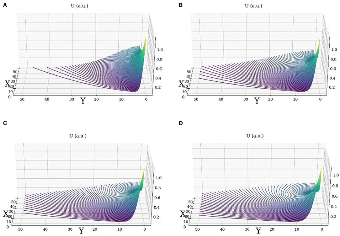
Figure 1. Normalized velocity field U, for θ = 180°; (A) ξ = 0.5; (B) ξ = 1; (C) ξ = 1.5; and (D) ξ = 2.

FIGURE 2

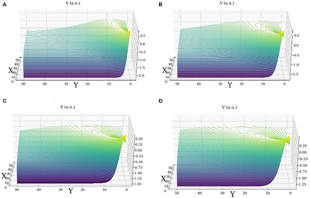
Figure 2. Normalized velocity field V, for θ = 180°; (A) ξ = 0.5; (B) ξ = 1; (C) ξ = 1.5; and (D) ξ = 2.

The above dependences specify the non-linearity behaviors of the velocity fields: a multifractal soliton for the velocity field across the Ox axis, respectively, “mixtures” of multifractal soliton—multifractal kink of the velocity fields across the Oy axis. The multifractality of the atmosphere dynamics is “explained” through its dependence from scale resolutions (Figures 1, 2).

The velocity fields (21) and (22) induces the multifractal minimal vortex

\begin{array}{l} Ω = (\frac{\partial U}{\partial Y} - \frac{\partial V}{\partial Y}) = \frac{0.57 Y}{{(ξ X)}^{2}} + \frac{0.63 ξ}{{(ξ X)}^{\frac{4}{3}}} t a n h [\frac{0.5 Y}{{(ξ X)}^{\frac{2}{3}}}] \\ + \frac{1.9 Y}{{(ξ X)}^{2}} s e c h^{2} [\frac{0.5 Y}{{(ξ X)}^{\frac{2}{3}}}] - \frac{0.57 Y}{{(ξ X)}^{2}} t a n h^{2} [\frac{0.5 Y}{{(ξ X)}^{\frac{2}{3}}}] \\ - [\frac{1.5}{{(ξ X)}^{\frac{2}{3}}} + \frac{1.4 Y^{2}}{X {(ξ X)}^{\frac{5}{3}}}] s e c h^{2} [\frac{0.5 Y}{{(ξ X)}^{\frac{2}{3}}}] t a n h [\frac{0.5 Y}{{(ξ X)}^{\frac{2}{3}}}], & (23) \end{array}

In Figures 3A–D the dependences of minimal vortex field Ω for various fractal degrees ξ and a given rotation angle θ is presented.

FIGURE 3

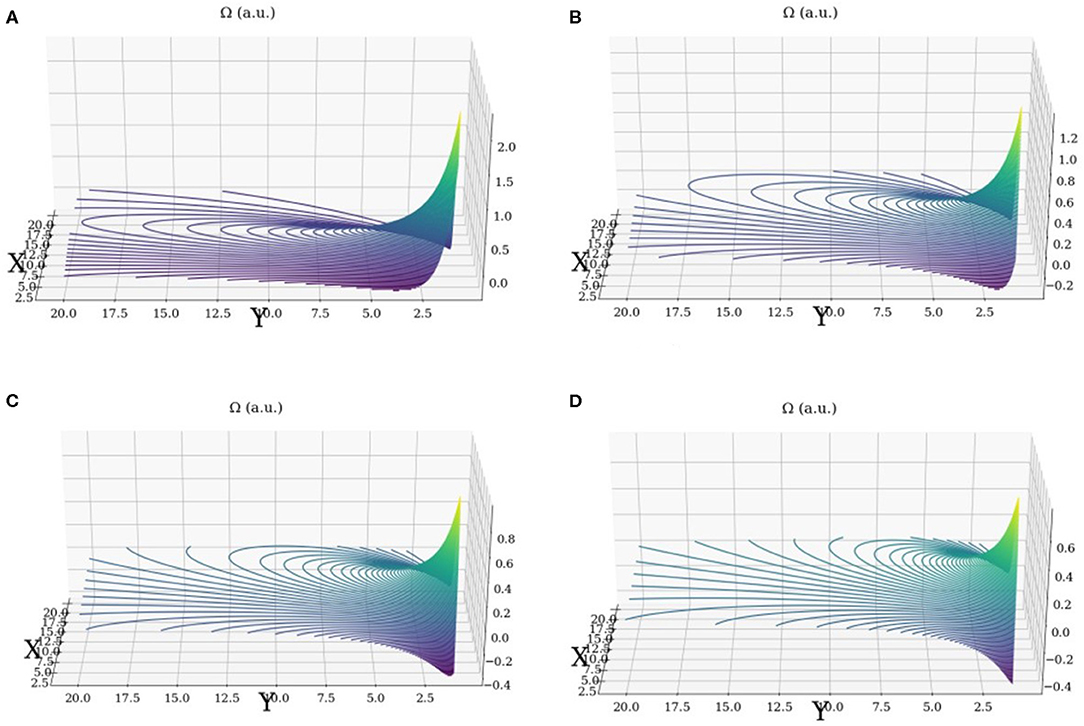
Figure 3. Multifractal minimal vortex field Ω, for θ = 180°; (A) ξ = 0.5; (B) ξ = 1; (C) ξ = 1.5; and (D) ξ = 2.

The above dependences specify the non-linear behaviors (through fractal degrees) of the minimal vortex field.

Energy Injection and Dissipation in Multifractal Turbulence

In turbulence, energy is injected in l₀ units, through a “cascade” of intermediary l_n scales, toward the dissipation scale l_d. We admit that this process can be described mathematically through the series of discrete scale lengths:

\begin{array}{l} l_{n} = 2^{- n} l_{0}, n = 0, 1, 2 \dots, & (24) \end{array}

given the associated wavenumbers:

\begin{array}{l} k_{n} = \frac{1}{l_{n}}, & (25) \end{array}

We follow with an analysis neglecting numerical factors, with the exception of those resulted from successive multiplications. Thus, if the specific kinetic energy of the “turbulent fluctuations” associated to the scale l_n is E_n, then it is possible to define by means of v_n as the average value of the velocity difference for l_n in the form:

\begin{array}{l} E_{n} = {v_{n}}^{2}, & (26) \end{array}

Then, the corresponding time interval can be defined as:

\begin{array}{l} t_{n} = \frac{l_{n}}{v_{n}}, & (27) \end{array}

We then admit that a certain fraction of the specific energy corresponding to the scale l_n is transferred to the scale l_n+1 during a period t_n. As a consequence, the specific energy transfer rate for n order units is given by the expression:

\begin{array}{l} ε_{n} = \frac{E_{n}}{t_{n}} = \frac{{v_{n}}^{3}}{l_{n}}, & (28) \end{array}

In the case of “stationary turbulence” the energy conservation law implies:

\begin{array}{l} ε_{n} = 〈 ε 〉, l_{0} > l_{n} > l_{d}, & (29) \end{array}

where 〈ε〉 is the average dissipation rate. We remind that 〈ε〉 found in (29) can be interpreted both as the rate of energy injection and the rate of energy transfer; the last is a relevant “measure” for the dynamics of the inertial domain. As regards the previous idea, we agree with the addressed Kraichnan critics (Kraichnan, 1974) of Kolmogorov modified models (Kolmogorov, 1962) observing that in these the central role of the dissipation is arbitrary as long as the specific energy conservation does not provide a connection between the local dissipation rate and local energy transfer rate. From (28) and (29) it results:

\begin{array}{l} v_{n} = {〈 ε 〉}^{\frac{1}{3}} {l_{n}}^{\frac{1}{3}}, & (30) \end{array}

and from (26) we obtain:

\begin{array}{l} E_{n} = {〈 ε 〉}^{\frac{2}{3}} {l_{n}}^{\frac{2}{3}}, & (31) \end{array}

an expression which, after Fourier transformation, is identical to its counterpart in Kolmogorov theory (Kolmogorov, 1962; McComb, 1990).

In the following let us consider the hypotheses that the average number of “vortex fragmentation” is N. Or, a scale unit l_n it is supposed to induce N subunits of scale l_n+1 for each value of n. Thus, the “fractional volume reduction,” from one “generation” to the others, is given by the equation:

\begin{array}{l} θ = \frac{N {l_{n + 1}}^{3}}{{l_{ϵ} n}^{3}} = \frac{N}{2^{3}} \leq 1, & (32) \end{array}

in which the second equality is explained through (24). Furthermore, if we admit that the largest units “fill” all the space they have at their disposal, then the n-th generation occupies the space:

\begin{array}{l} θ_{n} = θ^{n}, & (33) \end{array}

which will be occupied with units of scale l_n.

Now, we return to the previous argument, but limit ourselves to the “matter” volumes of n-th generation with a turbulent dynamic. Or, in these “regions,” (30) maintains its functionality. However, the relation between the globally averaged specific energy and locally averaged speed v_n is supposed to be:

\begin{array}{l} E_{n} = θ_{n} {v_{n}}^{2}, & (34) \end{array}

expressions which, by using the relations (30), (32), and (33) takes the form:

\begin{array}{l} E_{n} = {〈 ε 〉}^{\frac{2}{3}} {l_{n}}^{\frac{2}{3}} {(\frac{N}{2^{3}})}^{\frac{n}{3}}, & (35) \end{array}

Also, introducing:

\begin{array}{l} N = 2^{f (α)}, & (36) \end{array}

and the relation (24) to eliminate n, (35) can be written as:

\begin{array}{l} E_{n} = {〈 ε 〉}^{\frac{2}{3}} {l_{n}}^{\frac{2}{3}} {(\frac{l_{n}}{l_{0}})}^{- B (α)}, & (37) \end{array}

where we introduce the notation:

\begin{array}{l} B (α) = \frac{[f (α) - 3]}{3}, & (38) \end{array}

For an atmosphere with a mono-fractal behavior our model is reduced to the standard β model (Benzi et al., 1984; Paladin and Vulpiani, 1987; McComb, 1990).

Returning to the definition of the average turbulent energy dissipation rate, Tatarski finds the following definition for stationary atmospheric turbulence (Tatarski, 1961).

\begin{array}{l} ε ≅ 0.353 {l_{d}}^{2} Ω^{3}, & (39) \end{array}

Now, through (24), we can establish a number n such that the first, largest scale and the dissipation scale, are contained in the following equations:

\begin{array}{l} n_{l_{0}} = - {log}_{2} (\frac{l_{d}}{l_{0}}), & (40) \end{array}

In this manner, n_l₀ is the number of instances of vortices of l_n scales that are fractionated into an average of N subunits of l_n+1 scales in the energy cascade, starting from energy injection to dissipation. Using the relations (34) and (37) in this manner, combined with (40), we find:

\begin{array}{l} 〈 ε 〉 = 0.0441 \cdot (\frac{N^{\frac{3}{2}} {v_{l_{d}}}^{3}}{l_{0}}) \cdot 2^{[{log}_{2} (\frac{l_{d}}{l_{0}}) \cdot (\frac{{log}_{2} N - 5}{3})]}, & (41) \end{array}

\begin{array}{l} 〈 Ω 〉 ≅ \frac{1}{2} \cdot (\frac{\sqrt{N} v_{l_{d}}}{{l_{0}}^{\frac{1}{3}} {l_{d}}^{\frac{2}{3}}}) \cdot 2^{{\frac{1}{3} [{log}_{2} (\frac{l_{d}}{l_{0}}) \cdot (\frac{{log}_{2} N - 5}{3})]}}, & (42) \end{array}

where, v_{l_d} is the velocity difference between two points separated by l_d. Then, solving for N, it results:

\begin{array}{l} N ≅ 9.1895 \cdot {(\frac{{〈 Ω 〉}^{6} {l_{0}}^{4} {l_{d}}^{2}}{{v_{l_{d}}}^{6}})}^{\frac{1}{5}}, & (43) \end{array}

With (40) and (41) it is now possible to construct the expressions for the kinetic energy of the first and last “stages” of turbulent fluctuations, taking into consideration (35):

\begin{array}{l} E_{l_{0}} = 0.1248 \cdot {v_{l_{d}}}^{2} N {(\frac{l_{d}}{l_{0}})}^{[\frac{2}{9} (1.4426 ln N - 5)]}, & (44) \end{array}

\begin{array}{l} E_{l_{d}} = 0.1248 \cdot {v_{l_{d}}}^{2} N^{[1 - \frac{ln (\frac{l_{d}}{l_{0}})}{2.0799}]} {(\frac{l_{d}}{l_{0}})}^{[\frac{2}{9} (1.4426 ln N + 5)]}, & (45) \end{array}

The fraction $\frac{l_{d}}{l_{0}}$ is necessarily less than unity, so the shift of the “–” to a “+” sign will produce a smaller number; this gives the logical conclusion that E_{l_d} is necessarily smaller than E_l₀. In any case, between the liminal stages of the energy cascade, there are n stages with their own energy E_n, and all of them can be calculated in this manner, using only length scales and the average of the multifractal minimal vortex obtained by averaging obtained values in the vortex (Equation 23) in order to first obtain N (43).

Correspondences of the Model With Experimental Data

The introduction of the dissipation and injection scales is performed to verify equations with experimental data, and, by using experimental data to solve a number of these equations, to investigate the results. In the following segment of this paper, we present simulations of these various equations with a varying ξ non-dimensional parameter (Figures 1, 2), and we compare 〈ε〉 with measured data obtained via a lidar platform (Figure 6). For the sake of convenience, this theory used to construct ε(z) profiles with lidar data shall be referred to as the “Roşu-Tatarski method”; the finer details of this method are contained in a previous study (Rosu et al., 2019). This comparison is of qualitative nature; it is of interest to check if the profile yielded by theory in this study is comparable in evolution and order to a verified profile. Additionally, timeseries of 〈ε〉, n_l₀ and N altitude profiles are shown (Figures 7–9). The experimental data used to solve these equations is calculated by analyzing lidar RCS (Range Corrected Signal) data obtained and compiled on the 28th of May 2017 at the Optical Atmosphere Spectroscopy and Lasers Laboratory, part of the Faculty of Physics in the “Alexandru Ioan Cuza” University, at the coordinates 47.19306 North and 27.55556 East. The methodology for obtaining the injection and dissipation scale profiles is reliant on calculating the scintillation profiles of the lidar signal by observing the variation between multiple RCS profiles (Rosu et al., 2019).

The technical specifications of the main components of the lidar platform utilized in the study are as follows: the laser component is a Nd:YAG, producing pulses of laser at a frequency of 30 Hz, with a wavelength of 532 nm, laser beam diameter of 6 mm and a pulse energy of 100 mJ; meanwhile, the optical component is a Newtonian LightBridge telescope with a primary mirror diameter of 406 mm. The profiling frequency used in this particular study yielded 1 profile every minute. The lidar platform utilized in the study has a spatial resolution of 3.75 m and both technical details and results from previous measurement campaigns were reported in the scientific literature (Papayannis et al., 2014; Cazacu et al., 2018; Rosu et al., 2019). The profile is calculated by software written in Python 3.6 (Rosu et al., 2019). It must be mentioned that under 400 m AGL, calculations for the 〈ε〉 profile present many “mathematical domain errors,” which are visible as blank spaces in the timeseries; this may be a consequence of a number of factors, including a lack of sufficient computing power, instances of division by zero in the calculations, or others. The signal overlap altitude in most cases is at most 200 m from the lidar platform.

As mentioned, the length scale profiles used in this study are obtained by first calculating scintillation profiles in order to compile the structure coefficient of the refraction index profile $C_{N}^{2} (z)$ . According to Tatarski (1961), this can be calculated as:

\begin{array}{l} σ_{I}^{2} (L) = 1.23 C_{N}^{2} {(L) k}^{\frac{7}{6}} L^{\frac{11}{6}} & (46) \end{array}

with $σ_{I}^{2}$ being the scintilation (or, in this case, the logarithm of the standard deviation of light intensity) of a source of light observed from a distance represented by the optical path L. The definition:

\begin{array}{l} σ_{I}^{2} (L) = ln (1 + \frac{〈 {I (L)}^{2} 〉 - {〈 I (L) 〉}^{2}}{{〈 I (L) 〉}^{2}}), & (47) \end{array}

is given, with I(L) being the intensity of the range-corrected signal at the particular point in the optical path, which is analogous with the RCS intensity. Given the fact that the lidar platform produces 1 RCS profile every minute in this particular study, we have performed our averaging calculations necessary for the obtaining of the scintillation using 3 profiles. Thus, every 3 RCS profiles we obtain one 〈ε〉 for our timeseries, and an 〈ε〉, n_l₀ N, and profile is yielded every 3 min. Having determined the $C_{N}^{2} (z)$ profile, it is now possible to calculate, with or without a degree of approximation, the length scales. The inner scale profile is linked to scintillation (46) (Tatarski, 1961):

\begin{array}{l} σ_{I}^{2} (L) ≅ 0.615 C_{N}^{2} {(L) L}^{3} {l_{d} (L)}^{\frac{- 7}{3}}, & (48) \end{array}

while the outer scale is linked to the $C_{N}^{2} (z)$ profile (Tatarski, 1961):

\begin{array}{l} C_{N}^{2} (z) = {l_{0} (z)}^{\frac{4}{3}} {(\nabla \bar{n (z)})}^{2}, & (49) \end{array}

With turbulent eddies within the inertial subrange, the refraction index profile can be approximated from the definition of the respective structure coefficient (Tatarski, 1961; Yura, 1979):

\begin{array}{l} n (z) ≅ n_{0} - \sqrt{C_{N}^{2} (z) z^{\frac{2}{3}}}, & (50) \end{array}

which then gives us the means to extract the outer scale profile (49).

Regarding the potential influence of noise-related errors to the calculation of the scintillation profile used to obtain the length scales, the overall signal uncertainty added by noise is:

\begin{array}{l} Δ V = \sqrt{N S F^{2} (V - \bar{V_{b}}) + {(Δ V_{b})}^{2}}, & (51) \end{array}

where V is raw lidar signal, V_b is background lidar signal, and NSF is the “noise scale factor,” which is equal to the standard deviation of the shot noise divided by the square root of average shot noise (Liu et al., 2006). It is determined that the signal uncertainty, in the case of attenuated backscatter, has values of the order 10⁻⁷ or lower (Liu et al., 2006), while a typical attenuated backscatter profile has values of the order 10⁻⁵ or lower; thus, this uncertainty represents variations hundreds of times smaller than the actual values of the profile. Since the model subtracts the “dark” signal [generated by photocathode thermionic emission, which is collected before the measurements begin (Hamamatsu, 2007)] from the raw signal, we can assume that such uncertainty is even lower. Also, the fact that the photomultiplier component of the lidar platform utilized in this study was being operated in analog mode removes the need to consider possible instances of “afterpulsing,” which only take place when a photomultiplier component is operated in a “pulse detection mode” (Hamamatsu, 2007). Finally, the fact that the photomultiplier component of the lidar platform used in this study is a PMT (photomultiplier tube) presents an advantage, since excess noise decreases with an increase in the average photo-multiplication gain in PMTs (Liu et al., 2006).

First of all, velocity fields, the multifractal minimal vortex and its dissipation field are exemplified (Figures 1–4); the maximum intensity of the vortex lies close to the center, and as expected, the dissipation is also strongest there. Interestingly, the rotor structure presents a “downward-spiral” motion, wherein the minimum value and the maximum value are close to each other, and the trajectory from one to the other seems to be the shortest along the x-axis toward 0. The physical interpretation of this representation could be that it shows the manner in which the minimal vortex dissipates completely, with its kinetic energy being converted into internal energy. An increase in the non-dimensional parameter ξ produces a smaller minimum value in the vortex, and a “flatter” dissipation field (larger in size, with smaller values), however an increase in the parameter produces velocity fields that present a “sharper” peak and a more spread-out minimal region in a rotating manner. We assume that these simulated phenomena take place in relatively calm, from a meteorological perspective, ground-level conditions.

FIGURE 4

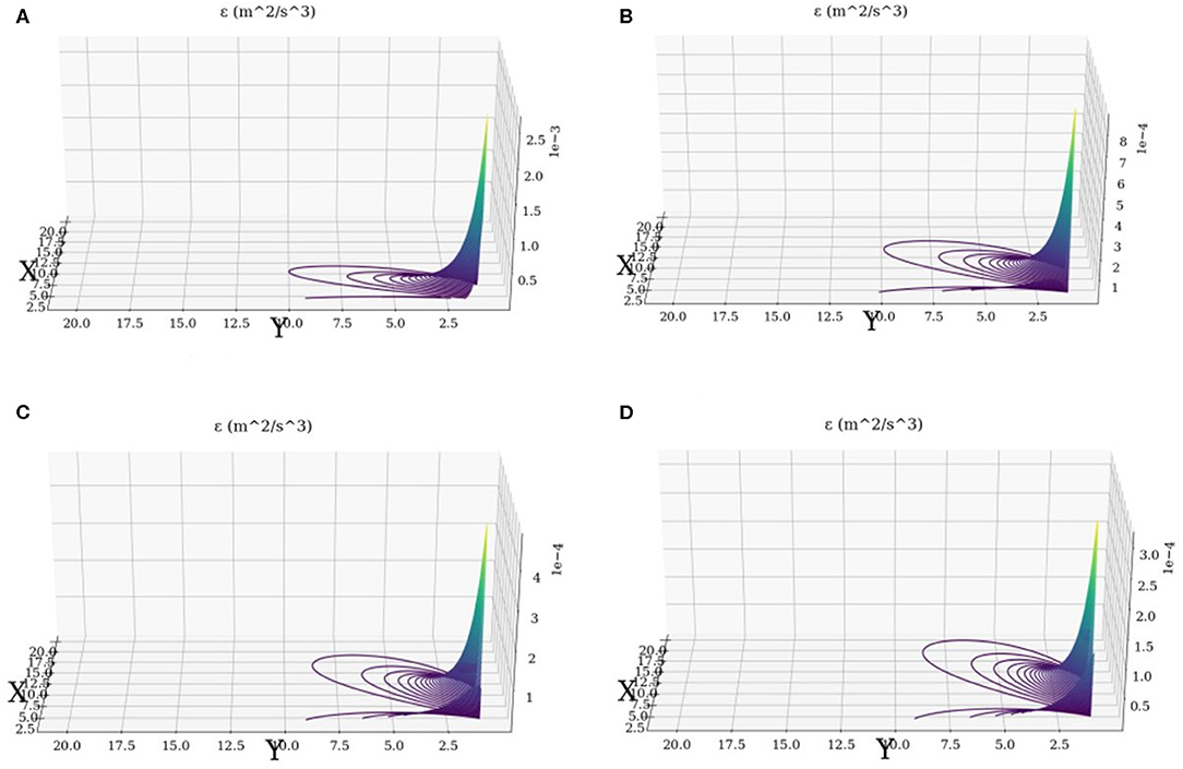
Figure 4. Turbulent dissipation rate field ε, for θ = 180°; (A) ξ = 0.5; (B) ξ = 1; (C) ξ = 1.5; and (D) ξ = 2.

The following figure is a timeseries of the RCS lidar signal used to calculate the length scales according to the presented theory (Figure 5); this figure is presented in order to ascertain with accuracy the location of the PBL (Planetary Boundary Layer) relative to values obtained in the rest of the timeseries. The comparison between 〈ε〉 obtained from this paper's theory and 〈ε〉 altitude profiles calculated through the Roşu-Tatarski method (Figure 6) seems to highlight many similarities. The two profiles are quite close in terms of numerical order and evolution, with the first 〈ε〉 profile exhibiting a more dynamical behavior than the lidar-obtained 〈ε〉 profile. Given that the first profile is calculated, through N (43), with just the average of the purely-theoretical multifractal minimal vortex and with the maximal and minimal length scales, these similarities are important.

FIGURE 5

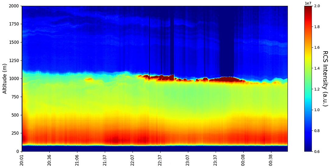
Figure 5. Lidar-obtained RCS timeseries on the 28th of May 2017; temporal resolution: 1 min; spatial resolution: 3.75 m.

FIGURE 6

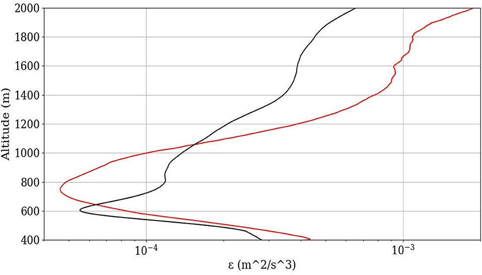
Figure 6. ε(z) profile (red) calculated with multifractal theory coupled with lidar-obtained length scales; ε(z) profile (black) calculated with Roşu -Tatarski method. Length scales profiled on the 28th of May 2017, 20:05.

Regarding the timeseries, 〈ε〉 values appear to be lowest in the region of the PBL (Figure 7); multiple studies seem to support the fact that turbulent dissipation is lowest at, or just above, the PBL, with both experimental and theoretical data (Chen, 1974; Shupe et al., 2012). The timeseries of N generally do not show values larger than 8 (Figure 8), which confirms the previously presented theory (32). Any values that may be slightly higher can be attributed to the various approximations taken throughout the theory, or to calculation errors, however in general the results seem to support the theory. The altitude variability of n_l₀ shown by the timeseries seems low, roughly between 14 and 17 (Figure 9); the equations do produce some non-integer results, which we can attribute once again to the taken approximations or calculation errors.

FIGURE 7

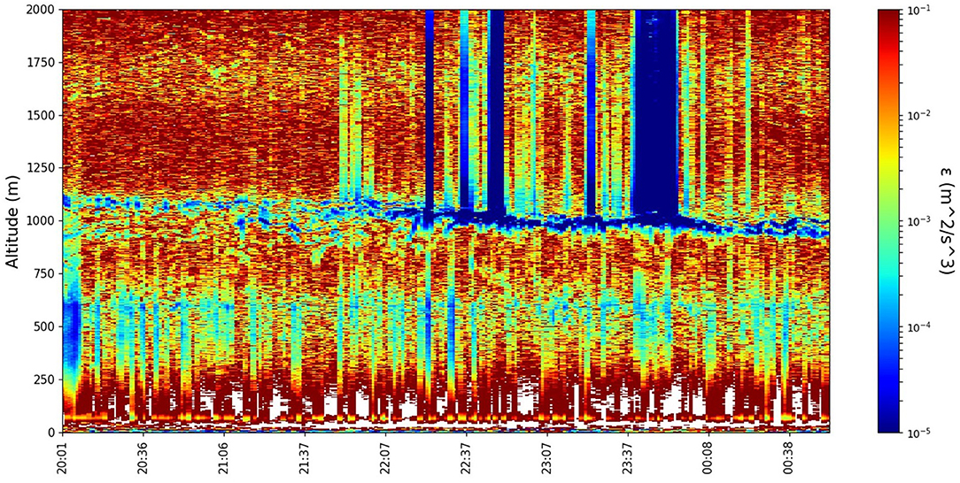
Figure 7. ε(z) timeseries on the 28th of May 2017 calculated with multifractal theory and lidar-obtained length scales; temporal resolution: 3 min; spatial resolution: 3.75 m.

FIGURE 8

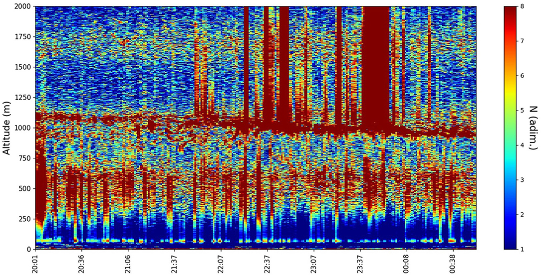
Figure 8. N(z) timeseries on the 28th of May 2017 calculated with multifractal theory and lidar-obtained length scales; temporal resolution: 3 min; spatial resolution: 3.75 m.

FIGURE 9

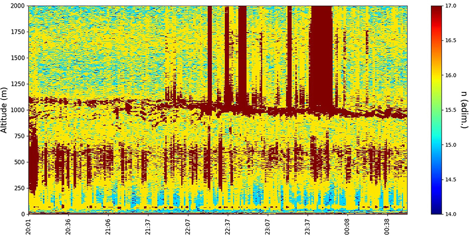
Figure 9. n(z) timeseries on the 28th of May 2017 calculated with multifractal theory and lidar-obtained length scales; temporal resolution: 3 min; spatial resolution: 3.75 m.

It must be highlighted that N and n_l₀ values seem highest in the PBL, with dissipation values being lowest. It is possible that this difference can be interpreted such that the turbulent behavior of the atmosphere in the PBL is more active, and more “resilient” to dissipative effects, which does indeed justify why this layer is such a stable and easily-recognizable feature of the atmosphere in most meteorological scenarios. The horizontal stripes of either very high or very low values in the time series, starting from certain intervals above the PBL, are produced due to signal noise present in the RCS lidar data used to calculate the length scales; this noise appears because of the influence of clouds in the vicinity of the PBL.

A simple analysis using a more discrete variation of the non-dimensional parameter ξ is also performed (Table 1); the maximal and minimal length scales used are l₀ = 260 m, l_d = 0.0035 m. First values of ξ for which N ≥ 8 are shown; it is found that realistic values of N are produced with ξ between 0.3 and 2.1. A number of important correlations can be inferred; some of these are obvious when analyzing the equations that dictate the parameters. First of all, a higher v_{l_d} produces a lower N; second of all, the dissipation seems to be more or less independent to N.

TABLE 1

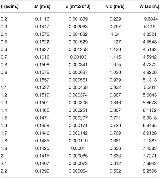
Table 1. Calculation of Ω, ε, v_{l_d}, and N with varying ξ.

Conclusions

In this work a holographic (multifractal) approach has been used to describe the non-linear behavior of the atmosphere, by considering that it can be assimilated to a complex system whose structural units support dynamics on continuous and non-differentiable curves. We have named this system the atmospheric multifractal, and the formulation of the motion operator of this atmospheric multifractal has allowed an analytic solution in the case of a plane symmetry for the dynamics of this system. The rotor of the obtained normalized velocity fields is then interpreted as the multifractal minimal vortex, which corresponds to the dissipation scale in the turbulent energy cascade. The velocity fields and the vortex are then plotted using multiple instances of a non-dimensional parameter that is linked to their fractal dimensions, and these results are discussed. Using this new formulation of the minimal vortex, it is then possible to extract an expression of turbulent energy dissipation in the atmospheric flow, and to construct an equation system that can describe the behavior of the cascade of vortices in terms of their scales, the average number of vortex fragmentations per “stage,” and the total number of stages of fragmentation, from injection to dissipation. In this equation system, from an atmospheric modeling and forecast point of view, the remaining unknown quantities are the injection and dissipation scales themselves; however, these quantities can be obtained as an atmospheric profile through a method detailed in one of our previous studies with a lidar platform. Using these profiles, time series of the turbulence parameters detailed in this study have been compiled, and it has been found that, especially regarding the known behavior of the PBL, they are in accord with the presented theory and existing scientific literature. Also, an altitude profile comparison has been made between turbulent energy dissipation calculated with the theory presented in this study and turbulent energy dissipation calculated with theory from one of our previous studies.

The success of these results leads us to believe that a future study might implement these theories, coupled with theoretical means of determining the inner and outer length scales, in order to produce forecasts of turbulent parameters; this, of course, using measured, ground-level, initial parameters. A future study might also include multiple other methods of experimentation and validation using platforms that would contain both traditional measurement instruments and remote sensing instruments. Finally, if these theories, along with many others, would be implemented into a fully functional model, a comparison with other well-known models could be performed in a potential new study.

Data Availability Statement

The datasets generated for this study are available on request to the corresponding author.

Author Contributions

IR, MC, MA, AG, and LB: conceptualization, formal analysis, original draft preparation, and visualization. IR, MC, and MA: methodology, validation, resources, data curation, writing—review and editing, supervision, and project administration. IR and MC: software and investigation and funding acquisition. All authors contributed to the article and approved the submitted version.

Funding

This work was supported by a research grant of the TUIASI, Project No. GnaC2018_65/2019.

Conflict of Interest

The authors declare that the research was conducted in the absence of any commercial or financial relationships that could be construed as a potential conflict of interest.

Supplementary Material

The Supplementary Material for this article can be found online at: https://www.frontiersin.org/articles/10.3389/feart.2020.00216/full#supplementary-material

References

Agop, M., and Paun, V. P. (2017). On the New Perspectives of Fractal Theory. Fundaments and Applications. Bucharest: Romanian Academy Publishing House, 101–110.

Arnold, V. I. (1980). Mathematical Models of the Classical Mechanics. Bucharest: Technical and Encyclopedical Publishing House (in Romanian), 256–327.

Badii, R. (1997). Complexity: Hierarchical Structures and Scaling in Physics. Cambridge University Press, 5–17. doi: 10.1017/CBO9780511524691

CrossRef Full Text | Google Scholar

Baker, G. L., and Gollub, J. P. (1996). Chaotic Dynamics: An Introduction. New York, NY: Cambridge University Press. 133–145. doi: 10.1017/CBO9781139170864

CrossRef Full Text | Google Scholar

Benzi, R., Paladin, G., Parisi, G., and Vulpiani, A. (1984). On the multifractal nature of fully developed turbulence and chaotic systems. J. Phys. A Math. Gen. 17:3521. doi: 10.1088/0305-4470/17/18/021

CrossRef Full Text | Google Scholar

Cazacu, M. M., Tudose, O., Balanici, D., and Balin, I. (2018). Research and development of commercial lidar systems in Romania: critical review of the ESYRO lidar systems developed by sc enviroscopy SRL (ESYRO). Eur. Phys. J. Conf. 176:11005. doi: 10.1051/epjconf/201817611005

CrossRef Full Text | Google Scholar

Chen, W. Y. (1974). Energy dissipation rates of free atmospheric turbulence. J. Atmos. Sci. 8, 2222–2225. doi: 10.1175/1520-0469(1974)031<2222:EDROFA>2.0.CO;2

CrossRef Full Text | Google Scholar

Cresson, J. (2007). Fractional embedding of differential operators and lagrangian systems. J. Math. Phys. 48:033504. doi: 10.1063/1.2483292

CrossRef Full Text | Google Scholar

Cristescu, C. P. (2008). Nonlinear Dynamics and Chaos. Theoretical Fundaments and Applications. Bucureşti: Romanian Academy Publishing House, 337–348.

Deville, M., and Gatski, T. B. (2012). Mathematical Modeling for Complex Fluids and Flows. Heidelberg: Springer. 150–161. doi: 10.1007/978-3-642-25295-2

CrossRef Full Text | Google Scholar

Hamamatsu. (2007). Photomultiplier Tubes, and Photomultipliers Tubes Photonics Basics and Applications. Iwata: Hamamatsu Photonics KK.

Hou, T. Y., Liu, C., and Liu, J. G. (2009). Multi-scale Phenomena in Complex Fluids: Modeling, Analysis and Numerical Simulations. Singapore: World Scientific Publishing Company, 156–163. doi: 10.1142/7291

CrossRef Full Text | Google Scholar

Kolmogorov, A. N. (1962). A refinement of previous hypotheses concerning the local structure of turbulence in a viscous incompressible fluid at high reynolds number. J. Fluid Mech. 13, 82–85. doi: 10.1017/S0022112062000518

CrossRef Full Text | Google Scholar

Kraichnan, R. H. (1974). On kolmogorov's inertial-range theories. J. Fluid Mech. 62, 305–330. doi: 10.1017/S002211207400070X

CrossRef Full Text | Google Scholar

Liu, Z., Hunt, W., Vaughan, M., Hostetler, C., McGill, M., Powell, K., et al. (2006). Estimating random errors due to shot noise in backscatter lidar observations. Appl. Opt. 45, 4437–4447. doi: 10.1364/AO.45.004437

PubMed Abstract | CrossRef Full Text | Google Scholar

Mandelbrot, B. B. (1982). The Fractal Geometry of Nature. San Fracisco, CA: W. H. Freeman and Co., 80–103.

PubMed Abstract | Google Scholar

McComb, W. D. (1990). The Physics of Fluid Turbulence. Oxford: Oxford Engineering Science Series, 93–113.

Google Scholar

Merches, I., and Agop, M. (2016). Differentiability and Fractality in Dynamics of Physical Systems. Singapore: World Scientific, 209–234. doi: 10.1142/9606

CrossRef Full Text | Google Scholar

Mitchell, M. (2009). Complexity: A Guided Tour. Oxford: Oxford University Press, 146–148.

Google Scholar

Nottale, L. (2011). Scale Relativity and Fractal Space-Time: A New Approach to Unifying Relativity and Quantum Mechanics. London: Imperial College Press, 403–425. doi: 10.1142/p752

CrossRef Full Text | Google Scholar

Ott, E. (2002). Chaos in Dynamical Systems. College Park, MD: Cambridge University Press, University of Maryland, 160–182. doi: 10.1017/CBO9780511803260

CrossRef Full Text | Google Scholar

Paladin, G., and Vulpiani, A. (1987). Anomalous scaling laws in multifractal objects. Phys. Rep. 156, 147–225. doi: 10.1016/0370-1573(87)90110-4

CrossRef Full Text | Google Scholar

Papayannis, A., Nicolae, D., Kokkalis, P., Binietoglou, I., Talianu, C., Belegante, L., et al. (2014). Optical, size and mass properties of mixed type aerosols in Greece and Romania as observed by synergy of lidar and sunphotometers in combination with model simulations: a case study. Sci. Total Environ. 500–501, 277–94. doi: 10.1016/j.scitotenv.2014.08.101

PubMed Abstract | CrossRef Full Text | Google Scholar

Rosu, I. A., Cazacu, M. M., Prelipceanu, O. S., and Agop, M. (2019). A turbulence-oriented approach to retrieve various atmospheric parameters using advanced lidar data processing techniques. Atmosphere 10:38. doi: 10.3390/atmos10010038

CrossRef Full Text | Google Scholar

Schlichting, H., and Gersten, K. (2017). Boundary-Layer Theory, 9th Edn. Berlin: Springer, 95–100. doi: 10.1007/978-3-662-52919-5

CrossRef Full Text | Google Scholar

Shupe, M. D., Brooks, I. M., and Canut, G. (2012). Evaluation of turbulent dissipation rate retrievals from doppler cloud radar. Atmos. Measure. Tech. 5, 1375–1385. doi: 10.5194/amt-5-1375-2012

PubMed Abstract | CrossRef Full Text | Google Scholar

Tatarski, V. I. (1961). Wave Propagation in a Turbulent Medium. Institute of Atmospheric Physics Academy of Sciences of the USSR Translated from Russian by R.A. Silverman. New York, NY: Dover Publications Inc.,208–211.

Google Scholar

van den Berg, J. C. (2004). Wavelets in Physics. Cambridge: Cambridge University Press, 143–147.

Google Scholar

Yura, H. T. (1979). Signal-to-noise ratio of heterodyne LIDAR systems in the presence of atmospheric turbulence. Opt. Acta Int. J. Opt. 26, 627–644. doi: 10.1080/713820039

CrossRef Full Text | Google Scholar

Keywords: turbulence, multifractal, atmosphere, non-differentiable, vortex, lidar, PBL

Citation: Roşu IA, Cazacu MM, Ghenadi AS, Bibire L and Agop M (2020) On a Multifractal Approach of Turbulent Atmosphere Dynamics. Front. Earth Sci. 8:216. doi: 10.3389/feart.2020.00216

Received: 09 February 2020; Accepted: 25 May 2020;
Published: 25 June 2020.

Edited by:

Valéry Masson, Météo-France, France

Reviewed by:

Eugen Radu, University of Aveiro, Portugal
Sergei Strijhak, Institute for System Programming (RAS), Russia
Iuliana Oprea, Colorado State University, United States

Copyright © 2020 Roşu, Cazacu, Ghenadi, Bibire and Agop. This is an open-access article distributed under the terms of the Creative Commons Attribution License (CC BY). The use, distribution or reproduction in other forums is permitted, provided the original author(s) and the copyright owner(s) are credited and that the original publication in this journal is cited, in accordance with accepted academic practice. No use, distribution or reproduction is permitted which does not comply with these terms.

*Correspondence: Marius Mihai Cazacu, cazacumarius@gmail.com

HYPOTHESIS AND THEORY article

On a Multifractal Approach of Turbulent Atmosphere Dynamics

Introduction

Mathematical Model

Results and Discussion

Dynamics of the Atmosphere at Non-differentiable Scale Resolution Through Hydronamic “Regimes”

Energy Injection and Dissipation in Multifractal Turbulence

Correspondences of the Model With Experimental Data

Conclusions

Data Availability Statement

Author Contributions

Funding

Conflict of Interest

Supplementary Material

References

People also looked at