

Abstract
Hosting over 10% of the world's population, low elevation (<10 m above mean sea-level) coastal zones are susceptible to saline groundwater intrusion—making fresh groundwater an often scarce and threatened commodity. To inform suitable coastal groundwater management strategies, regional-scale mapping of fresh and saline groundwater occurrence is extremely beneficial. This mapping is usually based on conventional ground-based methods. However, these are not only slow and expensive, but result in localized and disconnected information which is uneconomical and impractical on the larg scales required. Airborne electromagnetic (AEM) surveys have been proven a frugal and rapid way to overcome these shortcomings. Consequently, AEM methods are increasingly being used globally. Little is known about the effects of flightline spacing and additional ground-based data on the quality of mapping results, and in general the accuracy of AEM, other than validation against often sparse ground measurements. Understanding this is therefore invaluable as input to groundwater management strategies, survey planning and decision making. Here, we use a regional scale (900 km2), high-resolution (50 m × 50 m × 0.5 m) 3D synthetic model of electrical conductivity and geological properties, to investigate the effects of data availability on the accuracy of regional-scale groundwater salinity mapping. This was undertaken by simulating commonly used AEM parameters and realistic data acquisition methods. Two key data components are considered: (1) the AEM survey itself, and (2) geological information used to convert the AEM results into groundwater salinity. Spatially, different data-densities of these two components are quantitatively compared to highlight ideal geometrical configurations for given accuracy requirements. Our results indicate that in terms of optimising costs versus benefits, the value of additional lithological information is dependent on how well the initial distribution of electrical conductivity is resolved by the acquisition and inversion process.
Export citation and abstract BibTeX RIS

Original content from this work may be used under the terms of the Creative Commons Attribution 4.0 license. Any further distribution of this work must maintain attribution to the author(s) and the title of the work, journal citation and DOI.
1. Introduction
Despite comprising only ∼2% of global land area, low elevation (≤10 m above sea-level) coastal zones host ∼10% of the world's inhabitants, the majority of which are in developing countries (Neumann et al 2015). Coastal aquifers are consequently a high-demand and over-stressed water source (Post 2005). Unfortunately, these are susceptible to groundwater salinization (De Louw et al 2011), a problem worsened by excessive extraction and land-subsidence (Minderhoud et al 2017), which could be further aggravated by sea-level rise (Oude Essink et al 2010). Properly informed and vigilant management strategies are therefore crucial; thus accurate mapping of the regional-scale occurrence of fresh and saline groundwater is needed.
This mapping is traditionally based on conventional ground-based methods, which are not only slow and expensive, but result in localised and disconnected information which is uneconomical and impractical over the large areas required. Airborne electromagnetic (AEM) surveys have been proven a frugal and rapid way to overcome these shortcomings since the 1970s (Sengpiel 1981) and have since been successfully applied to map the distribution of groundwater salinity on regional scales (Fitterman and Deszcz-Pan 2001, Auken et al 2008, Faneca Sànchez et al 2012, Sulzbacher et al 2012, Jørgensen et al 2012, Siemon et al 2015, Delsman et al 2018, Meyer et al 2019). Primarily, two methods exist: time and frequency domain electromagnetics, referred to here as TEM and FEM respectively, and are discussed in detail and compared in Steuer et al (2009). Both methods operate by transmitting and receiving electrical signals from an instrument towed beneath a helicopter. The signals produce secondary currents in the subsurface which are in turn measured by receivers. The suitability of the method for coastal groundwater salinity mapping relates to electrical conductivity (EC) contrasts in the subsurface in the form of pore water salinity and clay content of host sediments (Mcneil 1980). Surveys are typically flown in a grid pattern at specified flightline spacing, resulting in observations every few meters downline.
Observations are normally represented as physical properties using inversions (Farquharson et al 2003, Auken et al 2005, Brodie and Sambridge 2006, Siemon et al 2009, Vignoli et al 2015, Hansen and Minsley 2019), where these produce a subsurface distribution of bulk electrical conductivity (ECb)—or rather the combined EC from two sources: lithology and pore water. Although ECb distributions are useful and can be used as a proxy to groundwater salinity distributions—or even used to automatically estimate a fresh-saline groundwater interface (Siemon et al 2018)—practical groundwater management requires quantitative salinity information. For this, pore water conductivity is needed (ECw), which can subsequently be transformed into chloride concentrations using empirical relationships (e.g. De Louw et al 2011). To acquire ECw from ECb, formation factors (FF) are used (Archie 1942) which requires geological information.
This is a serious source of uncertainty, as field measurements have shown that fresh groundwater in clay could have the same ECb values as brackish groundwater in sand (De Louw et al 2011). Thus, along with undertaking an AEM survey, potentially expensive and intrusive geological information is required for accurate transformation into groundwater salinity. Unlike many AEM mineral exploration programmes which aim to discern discrete or anomalous features of interest, hydrogeophysical mapping programmes tend to treat the entirety of the survey area with equal value, and thus a large scale and potentially expensive geological model is required.
Relatively few AEM studies have attempted to quantify regional groundwater salinity in 3D using FFs (e.g. Faneca Sànchez et al 2012, Delsman et al 2018, Vandevelde et al 2018). However, the recent success of hydrogeophysical groundwater investigations have resulted in increased attention to the method (Binley et al 2015). Current large-scale examples include plans for a potential a country-wide AEM survey across the Netherlands, and at the time of writing an unprecedently large AEM survey is currently being undertaken in Australia for mineral and groundwater mapping purposes (Ley-cooper et al 2018). In 2016 an atlas of subsurface EC was compiled throughout Denmark using primarily time-domain electromagnetics and ground data (Barfod et al 2016). Furthermore, recent methodological advances have allowed high-resolution provincial-scale 3D voxel models of groundwater salinity using probabilistic lithological and AEM derived ECb information (Delsman et al 2018). Consequently, it has become pertinent to better understand the groundwater salinity mapping error of AEM in general, as well as the effect of data density on mapping results. Although AEM has been tested and proven to be accurate and repeatable for both TEM (Foged et al 2013) and FEM systems (Huang and Cogbill 2006), currently little is known about the effects of flightline spacing and additional ground based data on the quality of 3D groundwater salinity mapping results. In general, model results are typically validated using 1D ground measurements (e.g. Faneca Sànchez et al 2012, Delsman et al 2018), but relative to an entire 3D regional model this only encompasses a very small region of the model space. Furthermore, physical differences in measurement techniques and acquisition conditions (e.g. temperature) mean that ground data are often difficult to directly compare with AEM. A quantitative and practical overview of the relative sources of error is therefore essential to inform the typically intra-disciplinary teams involved in AEM survey planning, decision making and ultimately groundwater management.
Consequently, in this paper we investigate relative sources of error based on established salinity mapping techniques using AEM with 3D models. Two key data types and their spatial configurations are considered: (1) the AEM survey itself and allocated flightline spacing, and (2) lithological information in the form of FF values through intrusive, ground-based drilling. Based on available subsurface data, this is undertaken using a large-scale (900 km2), high-resolution (50 × 50 × 0.5 m) model, extending to 50 m depth and comprising ∼150 million model cells and 90 separate model results.
To the authors' knowledge, a large-scale, fully 3D quantitative assessment of this nature is unique. We present the accuracy of results relating to three common mapping objectives: (1) error of the 3D model as a whole, (2) volume estimates and (3) fresh-saline interface depths. Results are presented in a practical manner as data densities per km2 and flightline spacing in meters apart and include current survey cost estimates to include economic considerations.
2. Methods
2.1. General approach
Our approach is summarized in six steps, and explained in order in sections 2.2 to 2.7: (1) synthetic data generation by transforming two existing 3D models (lithological and chloride) into an ECb volume; (2) simulate AEM acquisition using the ECb model (forward modelling) and subsequent inversion; (3) simulate lithological data collection from the 3D lithological model; (4) 3D interpolation of inversion results and lithological data; and (5) conversion to ECw and chloride by transforming interpolated results into ECw, and finally into 3D chloride models; (6) comparison with the synthetic chloride model and error analysis: finally, the estimated chloride estimates are compared against the synthetic model. Steps 2–6 are performed for different flightline spacings and different densities of ground-based information (geological drillings), where results are presented in section 3. The process is illustrated in figure S1 (stacks.iop.org/ERL/15/074002/mmedia). Hereafter, these steps are explained in more detail.
2.2. Step 1: synthetic data generation
The synthetic data is based on two existing high-resolution 3D datasets from southwestern Netherlands (figure 1). The latitudinally oriented Zeeuws-Vlaanderen strip (Zeelandic Flanders in English) covers an area of ∼60 × 15 km and lies within the southern edge of the North Sea basin. The shallow subsurface (up to ∼50 m) consists of gently northward dipping Neogene and Quaternary sediments (Stafleu et al 2011). Overall, lithologies comprise younger fine sands, clays and peats and deeper, gently dipping sands and silts (Vos 2015). Along the North Sea coast sandy coastal barriers are marked by localized topographic highs. Holocene sea-level transgressions caused extensive groundwater salinization (Delsman et al 2014) however subsequent land reclamation has allowed the formation of shallow freshwater lenses (Berendsen 2005). Given these events are recent in geological terms, distinct zones of fresh and saline groundwater with a relatively thin brackish zone are present throughout (Delsman et al 2018).

Figure 1. Data used to create the 3D synthetic model. 1A: flightlines and model area. 1B: 3D chloride model. 1C: lithological model. 1D: the resulting 3D ECb model used for forward modelling.
Download figure:
Standard image High-resolution imageThe chloride model used here (figure 1(b)) is the result of a provincial scale FEM survey that was flown in 2014/2015 in the Netherlands as a part of a research project called FRESHEM Zeeland (Delsman et al 2018). The resulting 3D groundwater salinity model is publicly available and has a resolution of 50 m horizontal and 0.5 m vertical, covering an area of ∼2000 km2. Specific details of survey parameters are available in Delsman et al (2018), and summarised in table 2. AEM surveys decrease in resolution at depth, therefore it should be noted that the 0.5 m resolution throughout the model is the result of a secondary interpolation step. In the study area the survey was flown at mostly 300 m line spacing, in areas of interest spacing was decreased to 100 m resulting in ∼3000 line km of HEM data. Flightlines are shown in figure 1(a). Flightline spacing is selected according to a compromise between target sizes and budget. Tie-lines are flown perpendicularly to these for data processing at a wider spacing.
A high-resolution 3D lithological voxel model (100 × 100 × 0.5 m resolution, up to 50 m depth from ground surface) of the area is available from the GeoTOP geological model as part of the Dutch national database of geological data (dinoloket.nl—accessed November 2016), and provided by the Geological Survey of the Netherlands (GSN-TNO). As well as a stratigraphic model, GSN-TNO's GeoTOP model contains the probability of lithoclasses occurring at any voxel and is therefore a probabilistic heterogeneous style model (lithoclasses and formation factors outlined in table 1 and shown in figure 1(c)). A more detailed description of the model is available in (Stafleu et al 2011). Apparent FF values were assigned to these lithologies and are based on nearby field measurements (De Louw et al 2011) (table 1). We recognize that the EC of saturated sediment is complex, such as surface conductivity caused by clay particles (Revil and Glover 1998), however for this work, we neglect the effect of the clay to surface conductivity since the exact values are heavily depended on the area of investigation (Revil et al 2017). Previous research examines this effect (Delsman et al 2018), but for this regional analysis we did not consider it an important factor.
Table 1. Lithological formation factor values used in this study, from De Louw et al (2011).
| Lithology | Formation factor (FF) |
|---|---|
| Peat | 2.1 |
| Clay | 2.5 |
| Sandy clay | 2.8 |
| Fine sand | 3.2 |
| Medium sand | 4 |
| Coarse sand | 5 |
Table 2. Simulated AEM system, survey and inversion parameters.
| Towed bird frequency domain system specifications | |
| Frequencies | 380, 1770, 8300, 41 000 and 129 500 Hz |
| Coil separation | ∼8 m |
| Coil orientations | 5 × horizontal coplanar |
| Measurement spacing | ∼40 m downline |
| Footprint | 100 m |
| Survey parameters | |
| Bird height | 40 m |
| Noise | 5% |
| Inversion parameters | |
| Vertical constraints | 1.3 |
| Lateral constraints | 3 |
To forward model (and subsequently invert) an AEM survey, a synthetic ECb model (i.e. the combined effect of both groundwater and lithology) is required. Using a combination of the two existing 3D models, a realistic and heterogeneous-style ECb model was created, the result of which is shown in figure 1(d). This process was undertaken in two steps: (1) the 3D chloride model was transformed to ECw using an empirical linear relationship from field measurements (De Louw et al 2011) and corrected back to a reference groundwater temperature of 11 °C from an initial 25 °C; (2) ECw was transformed into ECb by applying FF values based on the geological model. The resulting regional-scale 3D ECb synthetic model has a cell resolution of 50 m horizontal and 0.5 m vertical, covering an extent of ∼15 × 60 km down to 50 m depth from ground surface.
2.3. Step 2: simulate AEM acquisition
To simulate a typical survey across the 3D model, a distribution of measurement locations was needed. These were taken from the same survey that produced the 3D salinity model (Delsman et al 2018) in order to replicate typical heliborne survey characteristics (figure 1(a)). In total ∼800 000 measurements locations over 3000 line km were used from 361 flightlines, these were typically flown at between 100–300 m flightline spacing depending on the area. To facilitate processing times, the measurements were decimated to one every ∼40 m from every ∼4 m (totalling ∼100 000 measurements)—this was found to be a good balance between respecting the FEM system's ∼100 m footprint (Yin et al 2014) and hardware practicalities. Given that the signal measured by the AEM system is inherently 3D, and the forward modelling code used in this is paper is 1D (Auken et al 2005)—a pseudo-3D sampling technique was implemented. To achieve this, 100 m diameter circles were created around each measurement location to approximate the footprint of the FEM system (Yin et al 2014). Within each circle ECb was averaged, this was repeated at 0.5 m depth-slice intervals down to 50 m depth (i.e. at vertical model resolution), resulting in 100 000 synthetically generated AEM acquisition points on flight lines, each with 100 ECb values with depth (every 0.5 m until 50 m). Figure 2 illustrates the pseudo-3D sampling technique used, as well as an illustration of the resulting AEM coverage based on different flightline spacing.

Figure 2. The pseudo-3D sampling technique used to simulate the HEM system footprint. The effects of using different flightline spacing on coverage are illustrated.
Download figure:
Standard image High-resolution imageThe resulting data were forward modelled using AarhusINV (Auken et al 2005). Source and receiver spacing and frequencies were selected based on the RESOLVE HEM system; orientation was selected based on typical and previously used hydrogeophysical applications e.g. (Steuer et al 2009, Gunnink et al 2012, Delsman et al 2018). Finally, 5% random gaussian noise was added to the forward response to approximate HEM noise levels (Farquharson et al 2003, Green and Lane 2013).
The 'acquired' data, were inverted using AarhusINV (Auken et al 2005). Based on a commonly used inversion method (e.g. Auken et al 2008, Chongo et al 2015, Delsman et al 2018) and corresponding input parameters that were found suitable for hydrogeophysical studies (King et al 2018) (table 1), a laterally constrained inversion (LCI) was used (Auken and Christiansen 2004, Siemon et al 2009). The LCI method is a pseudo-2D method, whereby neighbouring model properties are constrained to produce laterally coherent inversion results along separate flightlines. The minimum-structure inversion style used here inverts for ECb values only, where layer thicknesses and depths remain constant, and has been found to accurately reproduce salinity distributions when compared with available ground data (King et al 2018, Delsman et al 2018).
The inversion starting model consisted of 20 layers, the thickness of the top layer was set to 0.68 m and subsequent layers increasing in thickness logarithmically until 50 m. Below 50 m the final layer is assumed to extend infinitely. A starting model conductivity of 1 S m−1 was selected based on common knowledge that low-lying coastal zones are (electrically) conductive environments.
2.4. Step 3: simulate lithological data collection
Simulating the acquisition of geological information, or indeed realistic quantities of existing data that may be available during hydrogeophysical mapping is not trivial. For example, the GeoTOP model used to construct the synthetic geological model in this paper is the result of expertly interpreted boreholes and geophysical data, resulting in a large-scale 3D probabilistic model with different properties (Stafleu et al 2011, Gunnink et al 2012). For this reason, a practical approach based on the current distribution of publicly available borehole data was used. Here we sampled synthetic borehole locations and depths from existing borehole data in the area available on Dinoloket, the Dutch Geological Survey (TNO) data portal. It was found that within the synthetic model area, cumulative vertical borehole depths totalled ∼42 000 m (or ∼60 vertical metres km−2), with a depth distribution highlighted in figure 3.
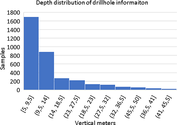
Figure 3. End-depth distribution of actual available lithological information on TNO's Dinoloket data portal.
Download figure:
Standard image High-resolution imageTypically, most available field data was found to be very shallow (<5 m), with very few holes deeper than ∼40 m. To replicate this characteristic, Inverse Transform Sampling (ITS) was used which iteratively generated a set of borehole depth values that matched this distribution. This was undertaken for a set of prescribed total vertical borehole depths in six total length classes as follows: 100 m (0.13 m km−2), 1000 m (1.36 m km−2), 5000 m (6.80 m km−2), 10 000 m (13.61 m km−2), 20 000 m (27.23 m km−2) and 42 000 m (57.19 m km−2)—based on practical criteria up to the actual amount available. Five ITS realisations were used for each total length class to account for sampling bias and to quantify uncertainty due to placement location. Finally, lithological classifications were sampled from the synthetic voxel model by each randomly selected borehole at 0.5 m vertical resolution till borehole depth. In effect drilling into the model and undertaking a full lithological interpretation. This resulted in 6 × 5 = 30 synthetic borehole datasets containing FF information. Here it is assumed that the process of transforming lithological information into apparent FF is free of instrument or human error.
2.5. Step 4: 3D interpolations of ECb inversion results and lithological data
In order to assess the effect of different flightline spacing on mapping results, the ECb inversions were subsequently split into three separate databases: (1) 300 m spacing, 100 m in specific areas (∼3000 line km), (2) 600 m flightline spacing (∼1500 line km), and (3) 1200 m spacing (∼750 line km). The 100 m line-spaced data was kept together with the 300 m, as this reflects a realistic data distribution and is the actual distribution of the original survey. This grouping allows an analysis of the effects of a higher AEM data density in specific areas. Finally, each database was interpolated into 3D volumes of ECb using the method of King et al (2018) and is based on 2D Kriging. We recognise that there are many other sophisticated methods to interpolate data, however this approach was found to accurately preserve the characteristics of inversion results between flightlines and offered a straightforward and recognised approach. The model base was assigned according to the DOI of the airborne system which varied between 5 to 60 m between conductive and resistive respectively, this was calculated from the inversion output at each 1D model location (Vest Christiansen and Auken 2012). Minimum-curvature gridding was then used to interpolate DOI estimates, data below these were removed from further analysis for all further models. A statistically robust, simple and repeatable 3D interpolation method was utilised to interpolate the FF values at the borehole data throughout the synthetic model. For this an established technique called Sequential Indicator Simulation (SIS) was used (Gomez-Hernandez and Strivastave 1990), based on Indicator formulation. Separate indicator semivariogram models were fitted for all six lithoclasses from each borehole iteration (a separate semivariogram model with different horizontal and vertical ranges for each of the 30 borehole datasets). For all 30 lithological spatial distributions, 10 SIS realisations were simulated. The median (or p50) of the 10 simulated lithologies at each model cell was used for further analysis, resulting in six FF value classes. The interpolation resulted in 30 3D lithological spatial distributions for which appropriate FF values were assigned (for each of the six classes of specified total drilling length with five randomised locations for each).
2.6. Step 5: conversion to ECw and chloride
Each of the 30 interpolated FF spatial distributions were multiplied by the three interpolated ECb inversion results to obtain 90 3D ECw spatial distributions (6 × 3 = 18 combinations of total borehole and flightline lengths with 5 random borehole sets per combination), which were then converted back to 3D chloride (as per figure S1).
2.7. Step 6: comparison with synthetic chloride model and error analysis
With practical hydrogeophysical mapping considerations in mind, the resulting 90 3D ECw spatial distribution models were compared against the synthetic model in three ways. All evaluations were undertaken over the same domain, where values beneath the calculated DOI from inversion results were removed. First, mean absolute error (MAE) of groundwater salinity estimates as mg l−1 chloride were calculated as per the following:
where xi is the prediction and x is the true value. Second, groundwater salinity volumes were calculated according to the chloride classifications set out by Stuyfzand (1986) and include the following: (1) 0–1000 mg l−1, or 'fresh', (2) 1000–3000 mg l−1, or 'brackish', and (3) >3000 mg l−1, or 'saline'. Finally, based on this classification, interface depths for the fresh-brackish-saline regions were extracted as 500, 1500 and 3000 mg l−1 chloride respectively. Saline inversion was present in some areas (saline above fresh groundwater), therefore multiple interfaces were frequently encountered at the same horizontal location. As a result, only the shallowest, or first encountered interfaces were extracted as iso-surfaces for further analysis.
3. Results
For clarity, geology refers to additional borehole information as vertical metres per km2; inversions refer to error as a result of the AEM acquisition and inversion process; and the reference model is the synthetic chloride model. In total all 90 3D chloride model properties of 150 million cells each (thus in total ∼13.5 billion data points) are compared in the following, relating to different geometrical data configurations of geological and AEM data. Volumes and interface error are calculated according to specified salinity classes, while MAE calculations focus on the entirety of the 3D models for an overview of error contributions. Uncertainty relating to borehole placement and 3D interpolation is shown as standard error.
3.1. MAE of salinity estimates
The mean absolute error (MAE) of mapped chloride is presented in figure 4, showing average error for all data configurations tested. To better isolate error per data type, in figure S2 we assumed a perfect inversion model and only adjusted the amount of lithological information.
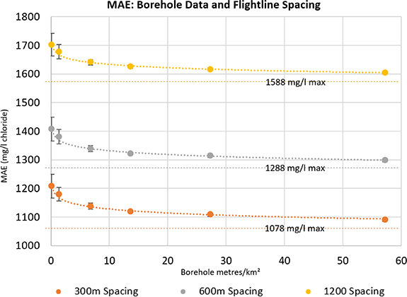
Figure 4. MAE of flightline spacing as meters apart vs. data density of borehole data as vertical meters drilled per km2. Yellow = 1200 m spacing, grey = 600 m spacing, orange = 300 m spacing; the vertical black error bars represent uncertainty range over the five sampled borehole configurations per borehole density class; the horizontal dashed lines are error due to AEM inversion only assuming perfect geological knowledge.
Download figure:
Standard image High-resolution imageFigure 4 illustrates that increasing borehole density to a value of more than ∼10 m km−2 results in relatively little improvement of mapped chloride. Geological data reduces mapping error by ∼100 mg l−1 chloride between the highest and lowest data densities for all flightline configurations and at maximum 150 mg l−1 chloride in case of perfect geological knowledge. Reducing flightline spacing consistently reduces error by ∼70 mg l−1 chloride per 100 m reduction. The reduction in salinity estimation error by adding geological information is significant if the AEM inversion is without error (figure S2), the combined error is dominated by the error in AEM inversion. Thus, the most effective way of reducing the error in chloride concentration mapping is by decreasing flightline spacing.
3.2. Volumes
Calculations were undertaken based on the classifications outlined in section 2.6, where a porosity factor of 0.3 was applied based on a sandy aquifer (Kirsch 2009), as the most commonly occurring sediment within the study area is fine sand. The result is a total groundwater volume of ∼5.71 × 10⁶ km3, with 3.13 × 10⁶ km3 (54%) fresh, 2.2 × 10⁶ km3 (39%) saline and 3.82 × 10⁵ km3 (6.7%) brackish groundwater volumes within the reference model. The AEM data acquisition and inversion process alone (assuming perfect geological knowledge) results in a substantial thickening of the brackish zone, adding ∼6.1 × 10⁵ km3 (10%) to brackish zone volume estimates (figure S4), underestimating the fresh and saline volume by ∼3.27 × 10⁵ km3 (4%) and ∼2.83 × 10⁵ km3 (6%) respectively. Figure 5 presents averaged volume differences against the reference model for each geological data density class with standard error (over the six borehole datasets per total borehole length class) and for a flightline distance of 300 m. Total error for each estimate has been subtracted by those of the reference model—thus positive values represent an overestimation.
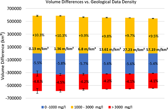
Figure 5. Differences in volume calculations against the reference model of fresh-brackish-saline groundwater regions using the 300 m line spaced survey. Km3 and percentage changes show relative change in volume for the entire model and are based on applying geological information (FF) to the inverted model (300 m line spacing). Blue = fresh, orange = brackish, red = saline. Borehole data density labelled as vertical metres km−2. Positive values represent an overestimation.
Download figure:
Standard image High-resolution imageResults for 600 m and 1200 m flightline distances share a similar magnitude of error. Figure S5 shows that if no AEM acquisition and inversion error is included, the reduction of errors in estimated volumes are notable. With less geological data a trend of overestimating the brackish zone at the expense of saline volumes is seen. Quantitatively, the addition of geological data reduces volume estimate error between the 0.13 m km−2 and 57.19 m km−2 borehole classes by ∼8.0 × 10³ km3 (0.3%), ∼4.0 × 10⁴ km3 (10.5%), and ∼5.0 × 10⁴ km3 (2.3%) for the fresh, brackish and saline classes respectively. It is clear however in figure S4, that that the inversion results in a significant overestimation of the brackish zone, therefore the addition of geological information reduces this error, but only marginally relative to the error introduced by the inversion.
The analysis of errors in volume estimates show that the largest error comes from the AEM acquisition and inversion method. Contrary to errors in salinity concentration estimates, over regional scales this error is not very sensitive to flightline spacing due to data averaging. Laterally less extensive features however, such as a small (1–2 km wide) fresh-water lens are likely to be more sensitive to this. Also, the reduction of the volume error from additional geological data is insignificant. Thus, if one is interested in estimating volumes of fresh, saline and brackish groundwater by airborne AEM, large flightline distances and little geological information is the most efficient option with the current methods of AEM acquisition and inversion.
3.3. Interfaces
When resolving the 500, 1500 and 3000 mg l−1 chloride interfaces, possible ECb values from inversion results may range between 0.06–0.13 S m−1, 0.11–0.25 S m−1 and 0.2–0.4 S m−1 respectively, in case the FF is unknown and between the values illustrated in figure S6. The result is that there exists an interface depth uncertainty range of a specified vertical thickness as a result of the inversion method used. As volume estimates show (figure S4), there is a significant smoothing effect from the inversion process—thus it follows that this will affect the thickness of the FF uncertainty range. This effect is demonstrated in cross-section, where the uncertainty limits are presented in figure 6 for the reference model and for the 300 m flightline spacing inversion model.
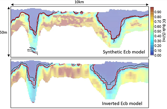
Figure 6. Upper (0.11 S m−1) and lower (0.25 S m−1) 1500 mg l−1 interface depth uncertainty ranges (black) for the synthetic ECb model and inverted ECb model, illustrated as a cross-section. The actual location of the interface in red.
Download figure:
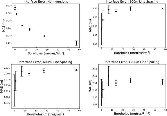
Standard image High-resolution imageFigure 6 highlights how the vertical uncertainty range is narrow (∼1.7 m MAE) in the synthetic ECb model, with substantial thickening (∼2.9 m MAE) in the inverted ECb model. It is also apparent that the inversion has caused the interface to become shallower overall, which is the result of an overestimation of the brackish zone by the inversion. To understand magnitude of the contribution of flightline distance and borehole density on the error in interface estimation, the MAE of interface positions against the reference model for the 1500 mg l−1 chloride are shown in figure 7. The 500 and 3000 mg l−1 chloride plots are supplied as supplementary information (figures S7 and S8).
Figure 7. Absolute vertical error of the 1500 mg l−1 chloride interface for each flightline spacing class, as well as a comparison directly against the reference model.
Download figure:
Standard image High-resolution image
Without the inversion, error margins are small (<0.5 m) for all interfaces and the addition of geology adds little improvement (between 0.05–0.1 m). The inversion and increasing flightline spacing however adds a more significant error to the mapping results: ∼3, 1.5 and 1 m for the 500, 1500 and 3000 mg l−1 chloride interfaces respectively. For every 300 m reduction in flightline spacing, approximately 0.1, 0.25 and 0.4 m of accuracy are added for 500, 1500 and 3000 mg l−1 chloride interfaces respectively—indicating that decreasing flightline spacing is useful for the more accurate delineation of deeper interfaces. However, the addition of geological information does little to help improve error and may even worsen it (for the 500 and 1500 mg l−1 interfaces). This contra-intuitive effect may be caused by the relatively large number of shallower boreholes, which resulted in an oversampling of clay lithologies that are predominantly close to the surface. As clay is has a lower FF (2.5), this results in more brackish groundwater to be unjustifiably classified as fresh and enhances the shallow bias in the 500 and 1000 mg l−1 interface depths. Naturally, this oversampling is more apparent when less lithological data are available.
4. Discussion and conclusions
We present a large-scale, quantitative study of groundwater salinity mapping accuracy using AEM. This study was undertaken using a high-resolution, 150 million cell synthetic 3D voxel model. We compared 90 possible 3D models, each of which was based on different data configurations of either geological data in the form of lithological logging, and as AEM in the form of flightline spacing. Commonly used and realistic data collection methods were simulated and interpolated into 3D groundwater salinity volumes. These volumes were then compared to the reference model to understand sources and quantities of error. The results are practical and useful as input to regional groundwater management strategies in coastal areas.
It was successfully demonstrated that a careful and systematic handling of the AEM acquisition and inversion process is the most important and cost-effective approach for accurate 3D groundwater salinity mapping using AEM. These findings support Delsman et al (2018) where the inversion process was the biggest uncertainty contributor to a 3D salinity model. The addition of ground-based geological information will help reduce error, but relatively insignificantly if the inversion process—and therefore the initial distribution of ECb—requires improvement.
As inversions are mathematically ill-posed, countless models can fit the observed data, thus selecting a single inversion that fits the data is not recommended, as demonstrated by Minsley (2011). Inversion error of groundwater salinity mapping was quantified by King et al (2018), where similar smoothing effects appeared to thicken the brackish zone—resulting in comparable fresh-saline interface mapping errors of ∼3 m. In this study ∼13.5 billion data points across 90 different 3D models were processed, therefore for practical reasons we used a single commonly used inversion method and parameters thereof. For the same reason we used a single interpolation method on the inversion results (King et al 2018), furthermore we found this suitable as it accurately preserved the thickness of the brackish zone between flightlines. Although testing different inversions and parameters would be interesting, this has been undertaken in a practical manner (Hodges and Siemon 2008, King et al 2018), and we feel that this study highlighted the importance of using inversion models carefully in general. Considering this, several methodological improvements could be suggested to constrain the thickness of the brackish zone; the simplest of which is to compare inversion methods and input parameters with accurate and direct ground-based ECb measurements. For example, if we know a narrow brackish zone exists from prior knowledge, the LCI sharp method (Vignoli et al 2015) could be used to try and match this characteristic. Hansen and Minsley (2019) offer a statistical approach that avoids the use of smoothing regularization constraints—such as the one that caused the thickening of the brackish zone in this study—and would allow the inclusion of explicit a-priori information.
Reducing flightline spacing reliably improved mapping results, particularly for salinity concentration mapping and mapping of salinity interfaces, and seemed to be the most efficient way of trading costs vs. accuracy. The economics involved in AEM surveys however are not straightforward and should be approximated with caution—for example, mobilisation and demobilisation costs mean that the price per line-km is non-linear and highly site-specific. For the sake of discussion however, as a coarse current estimate we could approximate €50 000 for mobilisation and €200 per line-km flown, including inverse modelling and full interpretation (Deltares, personal communication, September 2019). As a result, using these rough metrics the 300, 600 and 1200 m line spacing (or ∼3000, ∼1500, ∼750 line-km) survey results could total ∼€650 k, ∼€350 k, and ∼€200 k respectively.
To conclude, we showed that when mapping groundwater salinity using airborne EM (AEM) and ground based geological data, the error from AEM inversions far exceed that from errors in estimated formations factors (FF) obtained from lithological mapping. As a result, and given the estimated costs of AEM and geological drilling, decreasing flightline distances and producing high-quality inversion results are the most effective and efficient way of increasing the accuracy of groundwater salinity mapping, in particular when estimating salinity concentrations and the depth of interfaces between fresh and brackish groundwater. Volume estimates of the entire study area are however less sensitive to flightline distance. Overall results presented here allow a quantitative understanding of mapping error in large scale groundwater salinity mapping campaigns. This information is useful for the planning of regional groundwater mapping programmes using AEM in general. Results presented here are particularly useful for regional studies that share the characteristics of the realistic synthetic model, such as other low-elevation delta systems with sharp, shallow fresh-saline interfaces. In different hydrogeological terranes, a careful use of the inversion method remains equally important.
Acknowledgments
This research is financed by the Netherlands Organisation for Scientific Research (NWO), which is partly funded by the Ministry of Economic Affairs, and co-financed by the Netherlands Ministry of Infrastructure and Environment and partners of the Dutch Water Nexus consortium. Joeri van Engelen is acknowledged for his programming expertise, which allowed the automation of the forward and inverse modelling procedure.
Data availability
The data that support the findings of this study are available from the corresponding author upon reasonable request.