Abstract
Lambda-\({\mathcal {S}}\) is an extension to first-order lambda calculus unifying two approaches of non-cloning in quantum lambda-calculi. One is to forbid duplication of variables, while the other is to consider all lambda-terms as algebraic linear functions. The type system of Lambda-\({\mathcal {S}}\) has a constructor S such that a type A is considered as the base of a vector space while S(A) is its span. Lambda-\({\mathcal {S}}\) can also be seen as a language for the computational manipulation of vector spaces: The vector spaces axioms are given as a rewrite system, describing the computational steps to be performed. In this paper we give an abstract categorical semantics of Lambda-\({\mathcal {S}}^{*}\) (a fragment of Lambda-\({\mathcal {S}}\)), showing that S can be interpreted as the composition of two functors in an adjunction relation between a Cartesian category and an additive symmetric monoidal category. The right adjoint is a forgetful functor U, which is hidden in the language, and plays a central role in the computational reasoning.
1 Introduction
Algebraic lambda calculi aim to embed to the lambda calculus, the notion of vector spaces over programs. This way a linear combination \(\alpha .v+\beta .w\) of programs v and w, for some scalars \(\alpha \) and \(\beta \), is also a program [3]. This kind of construction has two independent origins. The Algebraic Lambda Calculus (ALC for short) [21] has been introduced as a fragment of the Differential Lambda Calculus [13], which is itself originated from Linear Logic [14]. ALC can be seen as the Differential Lambda Calculus without a differential operator. In the ALC the notion of vector spaces is embedded in the calculus with an equational theory, so the axioms of vector spaces, such as \(\alpha .v+\beta .v = (\alpha +\beta ).v\) are seen as equalities between programs. On the other hand, the Linear Algebraic Lambda Calculus (Lineal for short) [2] was meant for quantum computation. The aim of Lineal is to provide a computational definition of vector space and bilinear functions, and so, it defines the axioms of vector spaces as rewrite rules, providing a confluent calculus. This way, an equality such as \(-v+v+3.w-2.w = w\) is described computationally step by step as
Rules like \(\alpha .v+\beta .v\longrightarrow (\alpha +\beta ).v\) say that these expressions are not the same but one reduces to the other, and so, a computational step has been performed. The backbone of this computation can be described as having an element \(\alpha .v+\beta .v\) without properties, which is decomposed into its constituents parts \(\alpha \), \(\beta \), and v, and reconstructed in another way. Otherwise, if we consider \(\alpha .v+\beta .v\) being just a vector, as in the ALC, then it would be equal to \((\alpha +\beta ).v\) and the computation needed to arrive from the former to the latter would be ignored. The main idea in the present paper is to study the construction of Lineal from a categorical point of view, with an adjunction between a Cartesian closed category, which will treat the elements as not having properties, and an additive symmetric monoidal closed category, where the underlying properties will allow to do the needed algebraic manipulation. A concrete example is an adjunction between the category \(\mathbf {Set}\) of sets and the category \(\mathbf {Vec}\) of vector spaces. This way, a functor from \(\mathbf {Set}\) to \(\mathbf {Vec}\) will allow to do the needed manipulation, while a forgetful functor from \(\mathbf {Vec}\) to \(\mathbf {Set}\) will return the result of the computation.
The calculus Lambda-\({\mathcal {S}}\) [7, 8] is a first-order typed fragment of Lineal, extended with measurements. The type system has been designed as a quantum lambda calculus, where the main goal was to study the non-cloning restrictions. In quantum computing a known vector, such as a basis vector from the base considered for the measurements, can be duplicated freely (normally the duplication process is just a preparation of a new qubit in the same known basis state), while an unknown vector cannot. For this reason, a linear-logic like type system has been put in place. In linear logic we would write A the types of terms that cannot be duplicated while !A types duplicable terms. In Lambda-\({\mathcal {S}}\) instead A are the types of the terms that represent basis vectors, while S(A) are linear combinations of those (the span of A). Hence, A means that we can duplicate, while S(A) means that we cannot duplicate. Therefore, the S is not the same as the bang “!”, but somehow the opposite. This can be explained by the fact that linear logic is focused on the possibility of duplication, while here we focus on the possibility of superposition, which implies the impossibility of duplication.
In [7, 8] a first denotational semantics (in environment style) is given where the type \({\mathbb {B}}\) is interpreted as \(\{|0\rangle ,|1\rangle \}\) while \(S({\mathbb {B}})\) is interpreted as \(\mathsf {Span}(\{|0\rangle ,|1\rangle \})=\mathbb {C}^2\), and, in general, a type A is interpreted as a basis while S(A) is the vector space generated by such a basis. In [10, 11] we went further and gave a preliminary concrete categorical interpretation of Lambda-\({\mathcal {S}}\) where S is a functor of an adjunction between the category \(\mathbf {Set}\) and the category \(\mathbf {Vec}\). Explicitly, when we evaluate S we obtain formal finite linear combinations of elements of a set with complex numbers as coefficients and the other functor of the adjunction, U, allows us to forget the vectorial structure. In this paper, we define the abstract categorical semantics of the fragment of Lambda-\({\mathcal {S}}\) without measurement, which we may refer as Lambda-\({\mathcal {S}}^{*}\), so we focus on the computational definition of vector spaces, avoiding any interference produced by probabilistic constructions.
The main structural feature of our model is that it is expressive enough to describe the bridge between the property-less elements such as \(\alpha .v+\beta .v\), without any equational theory, and the result of its algebraic manipulation into \((\alpha +\beta ).v\), explicitly controlling its interaction. In the literature, intuitionistic linear (as in linear-logic) models are obtained by a monoidal comonad determined by a monoidal adjunction \((S,m)\dashv (U,n)\), i.e., the bang ! is interpreted by the comonad SU (see [4]). In a different way, a crucial ingredient of our model is to consider the monad US for the interpretation of S determined by a similar monoidal adjunction. This implies that on the one hand we have tight control of the Cartesian structure of the model (i.e. duplication, etc) and on the other hand the world of superpositions lives in some sense inside the classical world, i.e. determined externally by classical rules until we decide to explore it. This is given by the following composition of maps:
that allows us to operate in a monoidal structure explicitly allowing the algebraic manipulation and then to return to the Cartesian product.
This is different from linear logic, where the ! stops any algebraic manipulation, i.e. \(({!}{\mathbb {B}})\otimes ({!}{\mathbb {B}})\) is a product inside a monoidal category.
Outline. The paper is structured as follows.
-
Section 2 gives the intuition and formalization of the fragment of Lambda-\({\mathcal {S}}\) without measurements, called Lambda-\({\mathcal {S}}^{*}\), we give some examples, and state its main properties.
-
Section 3 presents the categorical construction for algebraic manipulation.
-
Section 4 gives a denotational semantics of Lambda-\({\mathcal {S}}^{*}\), using the categorical constructions from Sect. 3.
-
Section 4.2 proves the soundness and completeness of such semantics.
-
Finally, we conclude in Sect. 5. We also include an “Appendix” with detailed proofs.
2 The Calculus Lambda-\({\mathcal {S}}^{*}\)
In this section we define Lambda-\({\mathcal {S}}^{*}\), a fragment of Lambda-\({\mathcal {S}}\), without measurements. In addition, instead of considering the scalars in \(\mathbb {C}\), we use any commutative ring, which we will write \(\mathcal C\), so to make the system more general.
The syntax of terms and types is given in Fig. 1, where we write \({\mathbb {B}}^n\) for \({\mathbb {B}}\times \cdots \times {\mathbb {B}}\)n-times, with the convention that \({\mathbb {B}}^1={\mathbb {B}}\). We use capital Latin letters (\(A,B,C,\dots \)) for general types and the capital Greek letters \(\varPsi \), \(\varPhi \), \(\varXi \), and \(\Upsilon \) for qubit types. \(\mathcal B=\{{\mathbb {B}}^n\mid n\in \mathbb N\}\), \(\mathcal Q\) is the set of qubit types, and \(\mathcal T\) is the set of types (\(\mathcal B\subsetneq \mathcal Q\subsetneq \mathcal T\)). In the same way, \(\mathsf {Vars}\) is the set of variables, \(\mathsf B\) is the set of basis terms, \(\mathsf V\) the set of values, and \(\Lambda \) the set of terms. We have \(\mathsf {Vars}\subsetneq \mathsf B\subsetneq \mathsf V\subsetneq \Lambda \).

Syntax of types and terms of Lambda-\({\mathcal {S}}^{*}\)
The intuition of these syntaxes is given by considering \(\mathcal C=\mathbb {C}\). The type \({\mathbb {B}}\) is the type of a specific base of \(\mathbb {C}^2\), the base \(\{|0\rangle ,|1\rangle \}\), where we use the standard notation from quantum computing \(|0\rangle \) and \(|1\rangle \): \(|0\rangle \) denotes the vector \(\left( {\begin{matrix}1\\ 0\end{matrix}}\right) \) and \(|1\rangle \) denotes the vector \(\left( {\begin{matrix} 0\\ 1 \end{matrix}} \right) \). This way, \({\mathbb {B}}\times {\mathbb {B}}= \{|0\rangle \times |0\rangle ,|0\rangle \times |1\rangle ,|1\rangle \times |0\rangle ,|1\rangle \times |1\rangle \}\) is the base of \(\mathbb {C}^4\). The type \(S({\mathbb {B}})\) is the type of any vector in \(\mathbb {C}^2\), so S can be seen as the span operator. For example, \(2.|0\rangle +i.|1\rangle \) may live inside \(S({\mathbb {B}})\). On the other hand, a type of the form \({\mathbb {B}}\times S({\mathbb {B}})\) is the type of a pair of a base vector with a general vector, for example \(|0\rangle \times (\alpha .|0\rangle +\beta .|1\rangle )\) will have this type. There is no type for pair of function types, only pair of qubit types are considered. The type constructor S can be used on any type, for example, the type \(S({\mathbb {B}}\Rightarrow {\mathbb {B}})\) is a valid type which denotes the types of superpositions of functions, such as \(2.\lambda x{:}{\mathbb {B}}.x+3.\lambda x{:}{\mathbb {B}}.|0\rangle \). We will come back to the meaning of superposed functions later.
Terms are considered modulo associativity and commutativity of the syntactic symbol \(+\).
The term syntax is split in three: basis terms, which are values in the base of a vector space of values. Values, which are obtained by the formal linear combinations of basis terms, together with a null vector \(\mathbf {0}_{S(A)}\) associated to each type S(A). And a set \(\Lambda \) of general terms, which includes the values.
The syntax of terms contains:
-
The three basic terms for first-order lambda-calculus, namely, variables, abstractions and applications.
-
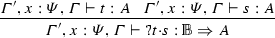
Two basic terms \(|0\rangle \) and \(|1\rangle \) to represent qubits, and one test \({}?{r}\mathord {\cdot }{s}\) on them. We may write \({t}?{r}\mathord {\cdot }{s}\) for \(({}?{r}\mathord {\cdot }{s})t\), see Example 2.1 for a clarification of why to choose this presentation.
-
A product \(\times \) to represent associative pairs (i.e. lists), with its destructors \(\text { head}\) and \(\text { tail}\). We may use the notation \(|b_1b_2\dots b_n\rangle \) for \(|b_1\rangle \times |b_2\rangle \times \dots \times |b_n\rangle \).
-
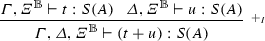
Constructors to write linear combinations of terms, namely \(+\) (sum) and . (scalar multiplication), without destructor (the destructor is the measuring operator, which we have explicitly left out of this presentation), and one null vector \(\mathbf {0}_{S(A)}\) for each type S(A).
-
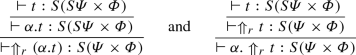
Two casting functions \(\Uparrow _r\) and \(\Uparrow _\ell \) which allows us to consider lists of superpositions as superpositions of lists (see Example 2.2).
The rewrite system has not yet been exposed, however the next examples give some intuitions and clarify the \({}?{r}\mathord {\cdot }{s}\) and the casting functions.
Example 2.1
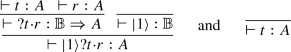
The term \({}?{r}\mathord {\cdot }{s}\) is meant to test whether the condition is \(|1\rangle \) or \(|0\rangle \). However, defining it as a function, allows us to use the algebraic linearity to implement the quantum-if [1]:
Example 2.2
The term \((\frac{1}{\sqrt{2}}(|0\rangle +|1\rangle ))\times |0\rangle \) is the encoding of the qubit \(\frac{1}{\sqrt{2}}(|0\rangle +|1\rangle )\otimes |0\rangle \). However, while the qubit \(\frac{1}{\sqrt{2}}(|0\rangle +|1\rangle )\otimes |0\rangle \) is equal to \(\frac{1}{\sqrt{2}}(|0\rangle \otimes |0\rangle +|1\rangle \otimes |0\rangle )\), the term will not rewrite to the encoding of it, unless a casting \(\Uparrow _r\) is preceding the term:
The reason is that we want the term \((\frac{1}{\sqrt{2}}(|0\rangle +|1\rangle ))\times |0\rangle \) to have type \(S({\mathbb {B}})\times {\mathbb {B}}\), highlighting the fact that the second qubit is a basis qubit, i.e. duplicable, while the term \(\frac{1}{\sqrt{2}}(|0\rangle \times |0\rangle +|1\rangle \times |0\rangle )\) will have type \(S({\mathbb {B}}\times {\mathbb {B}})\), showing that the full term is a superposition where no information can be extracted and hence, non-duplicable.
The rewrite system depends on types. Indeed, \(\lambda x{:}{S\varPsi }.t\) follows a call-by-name strategy, while \(\lambda x{:}{\mathbb {B}}.t\), which can duplicate its argument, must follow a call-by-base strategy [3], that is, not only the argument must be reduced first, but also it will distribute over linear combinations prior to \(\beta \)-reduction. Therefore, we give first the type system and then the rewrite system.
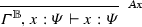
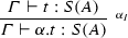
The typing relation is given in Fig. 2. Contexts, identified by the capital Greek letters \(\varGamma \), \(\varDelta \), and \(\varTheta \), are partial functions from \(\mathsf {Vars}\) to \(\mathcal T\). The contexts assigning only types in \(\mathcal B\) are identified with the super-index \({\mathbb {B}}\), e.g. \(\varTheta ^{\mathbb {B}}\). Whenever more than one context appear in a typing rule, their domains are considered pair-wise disjoint. Observe that all types are linear (as in linear-logic) except on basis types \({\mathbb {B}}^n\), which can be weakened and contracted (expressed by the common contexts \(\varTheta ^{\mathbb {B}}\)).
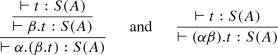
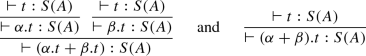
Notice that rule \(S_I\) makes type assignment not unique, since it makes possible to add as many S as wished. Also, there can be more than one type derivation tree assigning the same type, for example:


Typing relation
The rewrite relation is given in Figs. 3, 4, 5, 6, 7, 8, and 9.
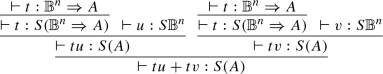
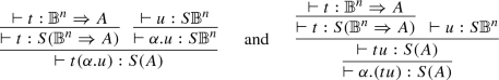
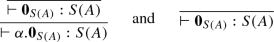
The two beta rules (Fig. 3) are applied according to the shape of the abstraction. If the abstraction expects an argument with a superposed type, then the reduction follows a call-by-name strategy (rule \(({\beta _{\mathsf {n}}})\)), while if the abstraction expects a basis type, the reduction is call-by-base (rule \(({\beta _{\mathsf {b}}})\)): it \(\beta \)-reduces only when its argument is a basis term. However, typing rules also allow to type an abstraction expecting an argument with basis type, applied to a term with superposed type (cf. Example 2.3). In this case, the \(\beta \)-reduction cannot occur and, instead, the application must distribute using the rules from Fig. 4: the linear distribution rules.

Beta rules

Linear distribution rules
Figure 5 gives the two rules for the conditional construction. Together with the linear distribution rules (cf. Fig. 4), these rules implement the quantum-if (cf. Example 2.1).

Rules of the conditional construction
Figure 6 gives the rules for lists, (\(\mathsf {head}\)) and (\(\mathsf {tail}\)).

Rules for lists
Figure 7 deals with the vector space structure implementing a directed version of the vector space axioms. The direction is chosen in order to yield a canonical form [2].

Rules implementing the vector space axioms
Figure 8 are the rules to implement the castings. The idea is that \(\times \) does not distribute with respect to \(+\), unless a casting allows such a distribution. This way, the types \({\mathbb {B}}\times S({\mathbb {B}})\) and \(S({\mathbb {B}}\times {\mathbb {B}})\) are different. Indeed, \(|0\rangle \times (|0\rangle +|1\rangle )\) has the first type but not the second, while \(|0\rangle \times |0\rangle +|0\rangle \times |1\rangle \) has the second type but not the first. This way, the first type give us the information that the state is separable, while the second type does not. We can choose to take the first state as a pair of qubits forgetting the separability information, by casting its type, in the same way as in certain programming languages an integer can be cast to a float (and so, forgetting the information that it was indeed an integer and not any float).
A second example is to take again Example 2.2: The term \(\frac{1}{\sqrt{2}}.(|0\rangle +|1\rangle )\times |0\rangle \) has type \(S({\mathbb {B}})\times {\mathbb {B}}\), expressing the fact that it is the composition of a superposed qubit with a basis qubit. However, the term \(\frac{1}{\sqrt{2}}.(|0\rangle \times |0\rangle +|1\rangle \times |0\rangle )\) has type \(S({\mathbb {B}}\times {\mathbb {B}})\), expressing the fact that it is a superposition of two qubits. The first type give us information about the separability of the two-qubits state, which is gathered from the fact that the term is indeed written as the product of two qubits. Contrarily, the second term is not the product of two qubits, and so the type cannot reflect its separability condition. In order to not lose subject reduction, we need to cast the first term so we “forget” its separability information, prior reduction.

Rules for castings \(\Uparrow _r\) and \(\Uparrow _\ell \)
Finally, Fig. 9 give the contextual rules implementing the call-by-value and call-by-name strategies.

Contextual rules
Example 2.3
The term \(\lambda x{:}{\mathbb {B}}.x\times x\) does not represent a cloning machine, but a CNOTFootnote 1 with an ancillary qubit \(|0\rangle \). Indeed,
The type derivation is as follows:

Example 2.4
A Hadamard gateFootnote 2 can be implemented by \(H=\lambda x{:}{\mathbb {B}}.{x}?{|-\rangle }\mathord {\cdot }{|+\rangle }\), where \(|+\rangle =\frac{1}{\sqrt{2}}.|0\rangle +\frac{1}{\sqrt{2}}.|1\rangle \) and \(|-\rangle =\frac{1}{\sqrt{2}}.|0\rangle -\frac{1}{\sqrt{2}}.|1\rangle \). Therefore, \(H:{\mathbb {B}}\Rightarrow S({\mathbb {B}})\) and we have \(H|0\rangle \longrightarrow ^*|+\rangle \) and \(H|1\rangle \longrightarrow ^*|-\rangle \).
Correctness has been established in previous works for slightly different versions of Lambda-\({\mathcal {S}}^{*}\), except for the case of confluence, which has only been proved for Lineal. Lineal can be seen as an untyped fragment without several constructions (in particular, without measurement), extended with higher-order computation. The proof of confluence for Lambda-\({\mathcal {S}}\) is delayed to future work, using the development of probabilistic confluence from [12]. The proof of Subject Reduction and Strong Normalization are straightforward modifications from the proofs of the different presentations of Lambda-\({\mathcal {S}}\).
Theorem 2.5
(Confluence of Lineal, [2, Thm. 7.25]) Lineal is confluent.
Theorem 2.6
(Subject reduction on closed terms, [8, Thm. 5.12]) For any closed terms t and r and type A, if \(t\longrightarrow r\) and \(\vdash t:A\), then \(\vdash r:A\).
Theorem 2.7
(Strong normalization, [8, Thm. 6.10]) If \(\varGamma \vdash t:A\) then t is strongly normalizing.
Why First Order The restriction on functions to be first order answers a technical issue with respect to the no-cloning property on quantum computing. Lambda-\({\mathcal {S}}\) is meant for quantum computing, and, in quantum computing, there is no universal cloning machine. Defining an affine type system, as we did, we avoid cloning machines such as \(\lambda x^{S({\mathbb {B}})}.x\times x\), which cannot be typed. However, with high order it would be possible to encode a cloning machine by encapsulating the term to be cloned inside a lambda abstraction, as in the following example:
First order ensures this cannot be done.
Since the calculus is first order, it adds atomic terms (\(|0\rangle \) and \(|1\rangle \)), and so, no need to encode those. Therefore, products of functions are not needed either, this is the reason why Lambda-\({\mathcal {S}}\) does not include them.
More Intuitions Despite that Lambda-\({\mathcal {S}}\) has been defined with quantum computation in mind, it can be seen just as a calculus to manipulate vector spaces. This is the feature that we want to highlight in this work, which is more general than just quantum computing. In particular, the derivation of \(v+(-1).v+3.w+(-2).w = w\) given in the introduction can be replicated with the rules from Lambda-\({\mathcal {S}}^{*}\) as follows.
Also, with the help of the casting, we can write step by step distributions between \(+\) and \(\otimes \). In Lambda-\({\mathcal {S}}^{*}\) we write \(\times \) instead of \(\otimes \) because it does not behave as a \(\otimes \) unless it is preceded by a casting \(\Uparrow \). For example, \(u\otimes (v+w) = (u\otimes v)+(u\otimes w)\), but \(u\times (v+w)\) does not reduce to \((u\times v)+(u\times w)\), unless the casting is present, in which case we have
3 A Categorical Construction for Algebraic Manipulation
3.1 Preliminaries
In this section, we recall certain basic concepts of the theory of categories and we establish a common notation that will help to define our work platform. For general preliminaries and notations on categories we refer to [19].
Definition 3.1
A symmetric monoidal category, also called tensor category, is a category \(\mathcal V\) with an identity object \(I\in \mathcal V\), a bifunctor \(\otimes :\mathcal V\times \mathcal V\rightarrow \mathcal V\) and natural isomorphisms \(\lambda :A\otimes I\rightarrow A\), \(\rho :I\otimes A\rightarrow A\), \(\alpha :A\otimes (B\otimes C)\rightarrow (A\otimes B)\otimes C\), \(\sigma :A\otimes B\rightarrow B\otimes A\) satisfying appropriate coherence axioms.
A symmetric monoidal closed category is a symmetric monoidal category \(\mathcal V\) for which each functor \(-\otimes B:\mathcal V\rightarrow \mathcal V\) has a right adjoint \([B,-]:\mathcal V\rightarrow \mathcal V\), i.e., \(\mathcal V(A\otimes B,C)\cong \mathcal V(A,[B,C])\).
Definition 3.2
A Cartesian category is a category admitting finite products (that is, products of a finite family of objects). Equivalently, a Cartesian category is a category admitting binary products and a terminal object (the product of the empty family of objects). A Cartesian category can be seen as a symmetric monoidal category with structural maps defined in an obvious way.
A Cartesian closed category is a Cartesian category \(\mathcal C\) which is closed as a symmetric monoidal category.
Definition 3.3
A symmetric monoidal functor \((F,m_{A,B},m_I)\) between symmetric monoidal categories \((\mathcal V,\otimes ,I,\alpha ,\rho ,\lambda ,\sigma )\) and \((\mathcal W,\otimes ',I',\alpha ',\rho ',\lambda ',\sigma ')\) is a functor \(F:\mathcal V\rightarrow \mathcal W\) equipped with morphisms \(m_{A,B}:FA\otimes 'FB\rightarrow F(A\otimes B)\) natural in A and B , and for the units morphism \(m_I:I'\rightarrow F(I)\) satisfying some coherence axioms. A monoidal functor is said to be strong when \(m_I\) and \(m_{A,B}\) for every A and B are isomorphisms and strict when all the \(m_{A,B}\) and \(m_I\) are identities.
Definition 3.4
A monoidal natural transformation \(\theta :(F,m)\rightarrow (G,n)\) between monoidal functors is a natural transformation \(\theta _A:FA\rightarrow GA\) such that the following axioms hold: \(n_{A,B}\circ (\theta _{A}\otimes '\theta _{B})=\theta _{A\otimes B}\circ m_{A,B}\) and \(\theta _I\circ m_I=n_I\).
Definition 3.5
Let \((\mathcal V,\otimes ,I)\) and \((\mathcal W, \otimes ', I')\) be monoidal categories. We say that \(((F,m),(G,n),\eta ,\varepsilon )\) is a monoidal adjunction if
-
\((F,G,\eta , \varepsilon )\) is an adjunction.
-
(F, m), (G, n) are monoidal functors
-
\(\eta :Id\Rightarrow G\circ F\) and \(\varepsilon :F\circ G\Rightarrow Id\) are monoidal natural transformations, as defined in Definition 3.4,

Definition 3.6
A preadditive category is a category \(\mathcal C\) together with an abelian group structure on each set \(\mathcal C(A,B)\) of morphisms, in such a way that the composition mappings
are group homomorphisms in each variable. We shall write the group structure additively.
An additive category is a preadditive category with a zero object and a binary biproduct.
Definition 3.7
An additive symmetric monoidal closed category is a category \((\mathcal V,\otimes ,\oplus )\) such that \((\mathcal V,\otimes )\) is a symmetric monoidal closed category, \((\mathcal V,\oplus )\) is an additive category, and \(\otimes \) is bi-additive.
3.2 Adjunction for Algebraic Manipulation
In this section we give the main categorical construction on this paper, which is the adjunction for algebraic manipulation.
Definition 3.8
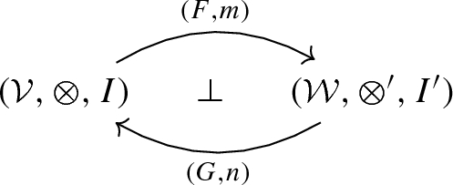
An adjunction for algebraic manipulation is a monoidal adjunction

where
-
\((\mathcal C,\times ,1)\) is a Cartesian closed category with 1 as a terminal object.
-
\((\mathcal V,\otimes ,\oplus ,\rho ,\lambda ,\sigma )\) is an additive symmetric monoidal closed category.
-
The following axiom (Axiom\(_{{}_0}\)) is satisfied for any f and g
where \(\mathbf 0\) is the zero morphism of the additive category.
-
The following axiom (Axiom\(_{{}_{\mathsf {Dist}}}\)) is satisfied
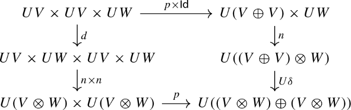
where
-
The map \(d:UV\times UV\times UW\longrightarrow UV\times UW\times UV\times UW\) is defined by \((\mathsf {Id}\times \sigma \times \mathsf {Id})\circ (\mathsf {Id}\times \varDelta )\).
-
The map \(\delta \) is an isomorphism determined by the fact that \(\otimes \) has a right adjoint. Explicitly, \(\delta :(V\oplus V)\otimes W\longrightarrow (V\otimes W)\oplus (V\otimes W)\) is given by \(\delta =\langle \pi _1\otimes \mathsf {Id},\pi _2\otimes \mathsf {Id}\rangle \).
-
The map p is an isomorphism determined by the preservation of product of the functor U given by the fact that U has a left adjoint. Explicitly, \(p_{V,W}:UV\times UW\longrightarrow U(V\oplus W)\) is given by \(p=\phi (\langle \phi ^{-1}(\pi _1),\phi ^{-1}(\pi _2) \rangle _{{}_{\mathcal V}})\) where \(\phi :\mathcal V(S(UV\times UW),V\oplus W)\cong \mathcal C(UV\times UW,U(V\oplus W))\), in which \(\pi _1:UV\times UW\longrightarrow UV\) and \(\pi _2:UV\times UW\longrightarrow UW\) are the projection maps.
-
-
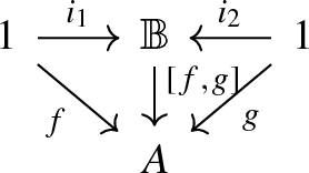
There exists an object \({\mathbb {B}}\in |\mathcal C|\) and maps \(i_1\), \(i_2\) such that for every \({1}\xrightarrow {f} A\) and \({1}\xrightarrow {g} A\), there exists a unique map \([f,g]\) such that the following diagram commutes


Remark 3.9
-
The object \({\mathbb {B}}\) allows us to represent the type \({\mathbb {B}}\), and the map \([f,g]\) to interpret the if construction (Definition 4.3).
-
\(\mathcal C\) is a Cartesian closed category where \(\eta ^A\) is the unit and \(\varepsilon ^A\) is the counit of \(-\times A\dashv [A,-]\), from which we can define the curryfication (\(\mathsf {curry}\)) and un-curryfication (\(\mathsf {uncurry}\)) of any map.
-
The adjunction \(S\dashv U\) gives rise to a monad \((T,\eta ,\mu )\) in the category \(\mathcal C\), where \(T=US\), \(\eta :\mathsf {Id}\rightarrow T\) is the unit of the adjunction, and using the counit \(\varepsilon \), we obtain \(\mu =U\varepsilon _S:TT\rightarrow T\), satisfying unity and associativity laws (see [19]).
-
Remember that in an additive category the morphism factoring through the zero object, i.e. the zero morphisms \(\mathbf 0\) are exactly the identities for the group structure in each \(\mathcal V(A,B)\) for every A and B.
-
Notice that since the tensor \(\otimes \) is bi-additive, it satisfies that \(f\otimes \mathbf 0=\mathbf 0\otimes f=\mathbf 0\) for every f.
Intuitively, the axiom Axiom\(_{{}_0}\) carries the absorbing property of the zero morphism, to the category \(\mathcal C\). Indeed, an analogous situation to this axiom, in the category \(\mathcal V\) is

which is valid since the dashed arrow makes the diagram commute. However, using the functor U we would obtain

which is less general than Axiom\(_{{}_0}\). Indeed, in Axiom\(_{{}_0}\) we allow the domain to be any A, and not necessarily of the form UW, capturing the absorbing property of a zero morphism, but in \(\mathcal C\).
The axiom Axiom\(_{{}_{\mathsf {Dist}}}\) gives us explicitly the intuition developed in the introduction. In the Cartesian category \(\mathcal C\) we do not have all the structure and properties as in the additive symmetric monoidal closed category \(\mathcal V\). However, we can mimic the distributivity property of \(\otimes \) with respect to \(\oplus \) by simply duplicating the last element and performing a permutation, i.e., \(\langle \langle a,b \rangle ,c \rangle \mapsto \langle \langle a,b \rangle ,\langle c,c \rangle \rangle \mapsto \langle \langle a,c \rangle ,\langle b,c \rangle \rangle \) mimic \((a\oplus b)\otimes c=(a\oplus c)\oplus (b\otimes c)\). While this property may be trivial when concrete categories are given, such as \(\mathbf {Set}\) for the Cartesian category and \(\mathbf {Vec}\) for the additive symmetric monoidal closed category, we have to axiomatize it in this abstract framework.
Example 3.10
One concrete model for Lambda-\({\mathcal {S}}^{*}\) has been briefly mentioned, which is the one presented in [10, 11]: an adjunction for algebraic manipulation where \(\mathcal C=\mathbf {Set}\) and \(\mathcal V=\mathbf {Vec}\).
We must prove that those categories satisfy the requirements from Definition 3.8.
-
Axiom\(_{{}_0}\) is satisfied for any f and g since the zero morphism is absorbing in \(\mathbf {Vec}\) and this property is preserved by U.
-
Axiom\(_{{}_{\mathsf {Dist}}}\) is satisfied since the concrete maps are the following:
$$\begin{aligned}&\langle a,b,c\rangle \mapsto \langle \langle a,b \rangle , c \rangle \mapsto \langle a,b \rangle \otimes c \mapsto \langle a\otimes c,b\otimes c \rangle \\&\langle a,b ,c\rangle \mapsto \langle a,c,b,c \rangle \mapsto \langle a\otimes c,b\otimes c \rangle \end{aligned}$$ -
We identify the object \({\mathbb {B}}\in |\mathbf {Set}|\) with \(\{|0\rangle ,|1\rangle \}\), which satisfies the required properties.
Example 3.11
More general, a family of examples is obtained by replacing Vec by a category \(\mathbf{Mod}_R\) of modules on a commutative ring R. The proof is essentially the same as the previous example.
Example 3.12
Let \((\mathcal C,\times ,1)\) be the category of sets \(\mathbf {Set}\) and \((\mathcal V,\otimes ,\oplus )\) be the category \(\mathbf {Ab}\) of abelian groups and group homomorphisms. These categories are cartesian and symmetric monoidal closed respectively. The tensor in \(\mathbf {Ab}\) is defined by a universal property, concretely, is the quotient of the free abelian group on the direct sum determined by the subgroup that satisfies some well-know relations and where \(I=\mathbb {Z}\). Also, \(\mathbf {Ab}\) is an additive category (see [5]). The functor S is the free construction \(S(X)= \{\{z_x\}_{x\in X}: z_x\in \mathbb {Z}; |\{x:z_x\ne 0\}|<\omega \}\) and U is the forgetful functor \(U:(\mathbf {Ab} ,\otimes _{\mathbb {Z} },\mathbb {Z} )\rightarrow (\mathbf {Set} ,\times ,\{*\}) \) where the mediating map \(n_{A , B} : U ( A )\times U ( B )\rightarrow U ( A \otimes B )\) sends \((a, b) \mapsto a \otimes b\) the map \(n_I:*\mapsto 1\).
Example 3.13
Let C be a cocommutative cosemisimple \(\mathbb {K}\)-coalgebra, where \(\mathbb {K}\) is a field. We consider \((\mathcal C,\times ,1)\) to be \(\mathcal C=\mathbf {Coalg/C}\) as the slice category of \(\mathbb {K}\)-cocommutative coalgebras and morphisms of coalgebras defined as follows: objects are morphisms of coalgebras with codomain in C, if \(\phi :D\rightarrow C\) and \(\psi :E\rightarrow C\) are morphisms of coalgebras (as object in the slice category), morphisms \(f:(\phi )\rightarrow (\psi )\) correspond to coalgebra morphisms \(f:D\rightarrow E\) such that \(\psi \circ f=\phi \). Cartesian product is given by pullbacks and \(1=id_C\) the identity morphism.
The structure \((\mathcal V,\otimes ,\oplus )\) is defined as follows: \(\mathcal V\) is the additive (abelian) category of C-comodules \(\mathbf{\mathcal {M}^C}\) (see [6]) such that the tensor is defined by an equalizer: Let (V, v) and (W, w) be C-comodules, where v and w are right coactions. There is a structure of C-comodule denoted by \(V\otimes ^C W\) in the vector space generated by \(\{x\otimes y \in V\otimes W\mid v(x)\otimes y=x\otimes \tau \left( w(y)\right) \}\) where the coaction is defined by \(\delta (x\otimes y)=x\otimes w(y)\) (see [16, 17]). If C is a cocommutative coalgebra, the category \((\mathbf{\mathcal {M}^C},\otimes ^C,C)\) is symmetric monoidal. Moreover, it is closed if and only if C is cosemisimple. (see [16, 17]). We define \(S:\mathbf {Coalg/C} \rightarrow \mathbf{\mathcal {M}^C}\) to be the functor that takes each object \(\phi :D\rightarrow C\) to the comodule (D, d), where \(d:D\rightarrow D\otimes C\) is the coaction defined by \(d=(id_D\otimes \phi ) \circ \varDelta _D\) and each morphism to its underlying morphism in \(\mathbf{\mathcal {M}^C}\). This functor is a strong monoidal functor and the existence of a right adjoint follows from the special adjoint functor theorem (see [16, 19]) which implies the existence of a monoidal adjunction (see [18]).
4 Denotational Semantics
4.1 Definitions
In this section we give the denotational semantics of Lambda-\({\mathcal {S}}^{*}\) by using the adjunction for algebraic manipulation defined in the previous section.
Definition 4.1
Types are interpreted in the category \(\mathcal C\), as follows:
Remark 4.2
To avoid cumbersome notation, we will use the following convention: We write directly USA for \(\llbracket {S(A)}\rrbracket =US\llbracket {A}\rrbracket \) and A for \(\llbracket {A}\rrbracket \), when there is no ambiguity.
In addition, we abuse notation and write \(\llbracket {\varGamma }\rrbracket \) for the product of the interpretations of all the types in \(\varGamma \). E.g. If \(\varGamma =x_1:\varPsi _1,\dots ,x_n:\varPsi _n\), then \(\llbracket {\varGamma }\rrbracket =\llbracket {\varPsi _1}\rrbracket \times \cdots \times \llbracket {\varPsi _n}\rrbracket \). We may write directly \(\varGamma \) for \(\llbracket {\varGamma }\rrbracket \), when there is no ambiguity.
Before giving the interpretation of typing derivation trees in the model, we need to define certain maps which will serve to implement some of the constructions in the language.
To implement the if construction we define the following map.
Definition 4.3
Given \(t,r\in \mathcal C(\varGamma ,A)\) there exists a map \(f_{t,r}\in \mathcal C({\mathbb {B}},[\varGamma ,A])\) defined by \(f_{t,r}= [\hat{t},\hat{r}]\) where \(\hat{t}\in \mathcal C(1,[\varGamma ,A])\) and \(\hat{r}\in \mathcal C(1,[\varGamma ,A])\) are given by \(\hat{t}=\mathsf {curry}(t\circ \pi _\varGamma )\) and \(\hat{s}=\mathsf {curry}(r\circ \pi _\varGamma )\).

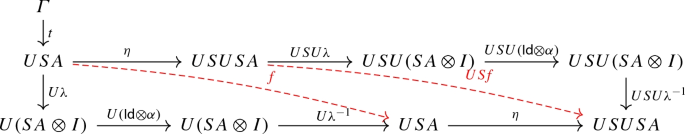
The sum in Lambda-\({\mathcal {S}}^{*}\) will be implemented internally by the map \(\nabla \) issued from the universal property of \(\oplus \). This way, we define a sum \(\hat{+}\) in \(\mathcal C\) as follows.
Definition 4.4
The map \(\hat{+}\) is defined by

where p has been defined in Definition 3.8.
The sum \(\hat{+}\) on \(USUV\times USUV\) is performed in the following way \(USUV\times USUV\xrightarrow {p} U(SUV\oplus SUV)\xrightarrow {U\nabla } USUV\). Notice that the map \(\nabla \) used in this construction is fundamentally different from the map \(\nabla \) defined over \(V\oplus V\). In order to perform all the sums at the same “level”, we would need to do \(USUV\times USUV\xrightarrow {g_1} US(UV\times UV)\xrightarrow {USp} USU(V\oplus V)\xrightarrow {USU\nabla }USUV\), where \(g_1\) factorizes the first US. We can generalize this idea to \((US)^kUV\times (US)^kUV\) with a map \(g_k\) factorizing the first k (US)s. Such a map is defined as follows.
Definition 4.5
The map \(g_k:(US)^{k}UV\times (US)^{k}UW\rightarrow (US)^k(UV\times UW)\) is defined by
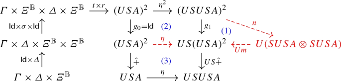
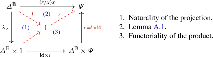
Example 4.6
We can define a map \(\mathsf {sum}\) on \(USUSUV\times USUSUV\) by using the sum \(\hat{+}\) on UV as \(USUS\hat{+}\circ g_2\), where \(g_2=(USUm)\circ (USn)\circ (Um)\circ n\). This gives the following diagram

The aim of the casting \(\Uparrow _r\) is to implement the distributivity property in \(\mathcal C\) by mapping \(USA\times B\) into \(US(A\times B)\). We want to perform such a property by using the underlying distributivity property in \(\mathcal V\).
In fact, the casting is defined more generally between \(US(USA\times B)\) and \(US(A\times B)\). A map denoting \(\Uparrow _r\) can be defined as follows.
Definition 4.7
Let \(\Uparrow _r^1\) be defined as follows

We generalize \(\Uparrow _r^1\) to the case \(US((US)^kA\times B)\) with the map \(\Uparrow ^k_r:US((US)^kA\times B)\rightarrow US(A\times B)\) is defined by
Analogously, we define \(\Uparrow ^k_\ell :US(A\times (US)^kB)\rightarrow US(A\times B)\).
Using all the previous definitions, we can finally give the interpretation of a type derivation tree in our model. If \(\varGamma \vdash t:A\) with a derivation \(\pi \), we write it generically \(\llbracket {\pi }\rrbracket \) as \(\varGamma \xrightarrow {t_A} A\). When A is clear from the context, we may write just t for \(t_A\). Also, each interpretation depends on a choice of scalars, i.e., a function \(c : \mathcal C\rightarrow \mathcal V(I,I)\); without loss of generality we denote the values \(c(\alpha )\) with the same letter \(\alpha \).
Definition 4.8
If \(\pi \) is a type derivation tree, we define \(\llbracket {\pi }\rrbracket \) inductively as follows,

4.2 Properties
In this section we prove that the given denotational semantics is sound (Theorem 4.11) and complete (Theorem 4.14).
Proposition 4.9 allows us to write the semantics of a sequent, independently of its derivation. Hence, due to this independence, we can write \(\llbracket {\varGamma \vdash t:A}\rrbracket \), without ambiguity.
Proposition 4.9
(Independence of derivation) If \(\varGamma \vdash t:A\) can be derived with two different derivations \(\pi \) and \(\pi '\), then \(\llbracket {\pi }\rrbracket =\llbracket {\pi '}\rrbracket \)
Proof
Without taking into account rules \(\Rightarrow _E\), \(\Rightarrow _{ES}\) and \(S_I\), the typing system is syntax directed. In the case of the application (rules \(\Rightarrow _E\) and \(\Rightarrow _{ES}\)), they can be interchanged only in a few specific cases.
Hence, we give a rewrite system on trees such that each time a rule \(S_I\) can be applied before or after another rule, we chose a direction to rewrite the tree to one of these forms. Similarly, we chose a direction for rules \(\Rightarrow _E\) and \(\Rightarrow _{ES}\). Then we prove that every rule preserves the semantics of the tree. This rewrite system is clearly confluent and normalizing, hence for each tree \(\pi \) we can take the semantics of its normal form, and so every sequent will have one way to calculate its semantics, i.e. as the semantics of the normal tree.
The full proof is given in the “Appendix”. \(\square \)
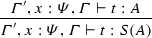
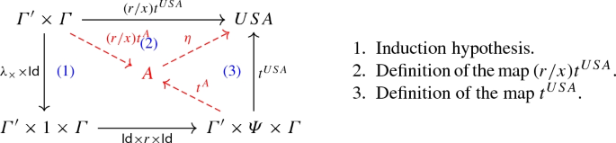
Lemma 4.10
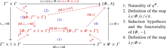
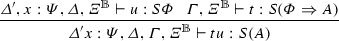
(Substitution) If \(\varGamma ',x:\varPsi ,\varGamma \vdash t:A\) and \(\vdash r:\varPsi \), then the following diagram commutes:

That is, \(\llbracket {\varGamma ',\varGamma \vdash (r/x)t:A}\rrbracket =\llbracket {\varGamma ',x:\varPsi ,\varGamma \vdash t:A}\rrbracket \circ (\llbracket {\vdash r:\varPsi }\rrbracket \times \mathsf {Id})\).
Proof
By induction on the derivation of \(\varGamma ',x:\varPsi ,\varGamma \vdash t:A\). The full proof is given in the “Appendix”. \(\square \)
Theorem 4.11
(Soundness) If \(\vdash t:A\), and \(t\longrightarrow r\), then \(\llbracket {\vdash t:A}\rrbracket = \llbracket {\vdash r:A}\rrbracket \).
Proof
By induction on the rewrite relation, using the first derivable type for each term. The full proof is given in the “Appendix”. \(\square \)
In order to prove completeness (Theorem 4.14), we use an adaptation to Lambda-\({\mathcal {S}}^{*}\) of Tait’s proof for strong normalization [20] (cf. [15, Chapter 6] for reference).
Definition 4.12
Let \(\mathcal A,\mathcal B\) be sets of closed terms. We define the following operators on them:
-
Closure by antireduction: \(\overline{\mathcal A}=\{t\mid t\longrightarrow ^*r_, \text { with }r\in \mathcal A \text { and }FV(t)=\emptyset \}\).
-
Product: \(\mathcal A\times \mathcal B=\{t\times u\mid t\in \mathcal A\text { and }u\in \mathcal B\}\).
-
Arrow: \(\mathcal A\Rightarrow \mathcal B=\{t\mid \forall u\in \mathcal A, tu\in \mathcal B\}\).
-
Span: \(S\mathcal A=\{\sum _i\alpha _ir_i\mid r_i\in \mathcal A\}\) where \(\alpha r\) is a notation for \(\alpha .r\) when \(\alpha \ne 1\), or 1.r or just r when \(\alpha =1\). Also, we use the convention that \(\sum _{i=1}^1\alpha _ir_i=\alpha _ir_i\) and \(0r=\mathbf {0}_{S(A)}\) for any r.
The set of computational closed terms of type A (denoted \(, A\)), is defined by
A substitution \(\sigma \) is valid with respect to a context \(\varGamma \) (notation \(\sigma \vDash \varGamma \)) if for each \(x:A\in \varGamma \), \(\sigma x\in , A\).
Lemma 4.13
(Adequacy) If \(\varGamma \vdash t:A\) and \(\sigma \vDash \varGamma \), then \(\sigma t\in , A\).
Proof
By induction on the derivation of \(\varGamma \vdash t:A\). The detailed proof can be found in the “Appendix”. \(\square \)
Theorem 4.14
(Completeness) If \(\llbracket {\vdash t:S({\mathbb {B}}^n)}\rrbracket =\llbracket {\vdash r:S({\mathbb {B}}^n)}\rrbracket \), then for any concrete model interpretation injective on values there exists s such that \(t\longrightarrow ^* s\) and \(r\longrightarrow ^*s\).
Proof
By Lemma 4.13, \(t\in , {S({\mathbb {B}}^n)}=\overline{S, {{\mathbb {B}}^n}}=\overline{S(\overline{{\mathbb {B}}^n})}\). Hence, \(t\longrightarrow ^*\psi \), with \(\vdash \psi :S({\mathbb {B}}^n)\) and \(\psi =\sum _i\alpha _i|b_{i1}\rangle \times \dots \times |b_{in}\rangle \). Then, by Theorem 4.11, \(\llbracket {\vdash t:S({\mathbb {B}}^n)}\rrbracket =\llbracket {\vdash \psi :S({\mathbb {B}}^n)}\rrbracket \). Analogously, \(r\longrightarrow ^*\phi \) and so by Theorem 4.11, \(\llbracket {\vdash r:S({\mathbb {B}}^n)}\rrbracket =\llbracket {\vdash \phi :S({\mathbb {B}}^n)}\rrbracket \), with \(\phi =\sum _j\beta _j|b_{j1}\rangle \times \dots \times |b_{jn}\rangle \). Therefore, since \(\llbracket {\vdash t:S({\mathbb {B}}^n)}\rrbracket =\llbracket {\vdash r:S({\mathbb {B}}^n)}\rrbracket \), we have \(\llbracket {\vdash \psi :S({\mathbb {B}}^n)}\rrbracket =\llbracket {\vdash \phi :S({\mathbb {B}}^n)}\rrbracket \), and so, since the model is injective on values, we have \(\psi =\phi =s\). \(\square \)
Remark 4.15
It is easy to verify that the model from Example 3.10 is injective on values, and hence, the model is Complete (Theorem 4.14).
On the other hand, there exist non injective concrete models. An easy example is the degenerated concrete model where both \(\mathcal C\) and \(\mathcal V\) are the terminal category (the category with a unique object and morphism), which is trivially both, Cartesian closed, and additive symmetric monoidal closed, and both axioms are satisfied trivially.
5 Conclusion
In this paper, we have given an abstract categorical semantics of Lambda-\({\mathcal {S}}^{*}\), a fragment of Lambda-\({\mathcal {S}}\) without measurements, and we have proved that it is sound (Theorem 4.11) and complete (Theorem 4.14). Such a semantics highlights the dynamics of the calculus: The algebraic rewriting (linear distribution, vector space axioms, and typing casts rules) emphasize the standard behavior of vector spaces, in a computational way: the vector space axioms give rise to computational steps. We have enforced this computational steps by interpreting the calculus into a Cartesian category \(\mathcal C\), without distributivity properties, and defining and using an adjunction for algebraic manipulation between this category \(\mathcal C\) and an additive symmetric monoidal closed category \(\mathcal V\) with all the properties needed for the vectorial space axioms. This way, in order to transform an element from the category \(\mathcal C\), we use the adjunction to carry these elements to \(\mathcal V\), where the proper transformation properties are in place.
As an immediate future work, we are willing to pursue a complete semantics for quantum computing, for which we need to add back the measurement operator, and define a notion of a norm, maybe following [9].
Notes
The CNOT quantum gate is such that CNOT\(|0x\rangle =|0x\rangle \) and CNOT\(|1x\rangle =|1\overline{x}\rangle \). Therefore, \(\mathrm {CNOT}(\alpha .|0\rangle +\beta .|1\rangle )|0\rangle =\alpha .\mathrm {CNOT}|00\rangle +\beta .\mathrm {CNOT}|10\rangle =\alpha .|00\rangle +\beta .|11\rangle \).
The Hadamard quantum gate is such that \(H|0\rangle =\frac{1}{\sqrt{2}}(|0\rangle +|1\rangle )\) and \(H|1\rangle =\frac{1}{\sqrt{2}}(|0\rangle -|1\rangle )\).
References
Altenkirch, T., Grattage, J.: A functional quantum programming language. In: Proceedings of the 20th Annual IEEE Symposium on Logic in Computer Science (LICS), pp. 249–258. IEEE (2005)
Arrighi, P., Dowek, G.: Lineal: a linear-algebraic lambda-calculus. Logical Methods in Computer Science 13(1:8) (2017)
Assaf, A., Díaz-Caro, A., Perdrix, S., Tasson, C., Valiron, B.: Call-by-value, call-by-name and the vectorial behaviour of the algebraic \(\lambda \)-calculus. Logical Methods in Computer Science 10(4:8) (2014)
Benton, N.: A mixed linear and non-linear logic: proofs, terms and models. In: Pacholski, L., Tiuryn, J. (eds.) Computer Science Logic (CSL 1994). Lecture Notes in Computer Science, vol. 933, pp. 121–135. Springer, Berlin (1994)
Borceux, F.: Handbook of Categorical Algebra, Encyclopedia of Mathematics and Applications, vol. 50. Cambridge University Press, Cambridge (2008)
Dascalescu, S., Nastasescu, C., Raianu, S.: Hopf Algebras: an Introduction. Pure and Applied Mathematics. A Series of Monographs and Textbooks. CRC Press, Boca Raton (2000)
Díaz-Caro, A., Dowek, G.: Typing quantum superpositions and measurement. Theory and Practice of Natural Computing (TPNC 2017). Lecture Notes in Computer Science, vol. 10687, pp. 281–293. Springer, Cham (2017)
Díaz-Caro, A., Dowek, G., Rinaldi, J.: Two linearities for quantum computing in the lambda calculus. BioSystems 186, 104012 (2019)
Díaz-Caro, A., Guillermo, M., Miquel, A., Valiron, B.: Realizability in the unitary sphere. In: Proceedings of the 34th Annual ACM/IEEE Symposium on Logic in Computer Science (LICS 2019), pp. 1–13 (2019)
Díaz-Caro, A., Malherbe, O.: A concrete categorical semantics for Lambda-\({\cal{S}}\). In: Logical and Semantic Frameworks with Applications (LSFA’18), Electronic Notes in Theoretical Computer Science, vol. 344, pp. 83–100 (2019)
Díaz-Caro, A., Malherbe, O.: A fully abstract model for quantum controlled lambda calculus. Draft at arXiv:1806.09236 (2020)
Díaz-Caro, A., Martínez, G.: Confluence in probabilistic rewriting. In: Logical and Semantic Frameworks with Applications (LSFA 2017), Electronic Notes in Teoretical Computer Science, vol. 338, pp. 115–131 (2018)
Ehrhard, T., Regnier, L.: The differential lambda-calculus. Theor. Comput. Sci. 309(1), 1–41 (2003)
Girard, J.Y.: Linear logic. Theor. Comput. Sci. 50, 1–102 (1987)
Girard, J.Y., Taylor, P., Lafont, Y.: Proofs and Types. Cambridge University Press, Cambridge (1989)
Grunenfelder, L., Paré, R.: Families parametrized by coalgebras. J. Algebra 107(2), 316–375 (1987)
Haim, M., Malherbe, O.: Linear hyperdoctrines and comodules. arXiv:1612.06602 (2016)
Kelly, G.: Doctrinal Adjunction. Category Seminar, Lectures Notes in Mathematics 420, 257–280 (1974)
Mac Lane, S.: Categories for the Working Mathematician, 2nd edn. Springer, Berlin (1998)
Tait, W.W.: Intensional interpretations of functionals of finite type I. J. Symb. Log. 32(2), 198–212 (1967)
Vaux, L.: The algebraic lambda calculus. Math. Struct. Comput. Sci. 19, 1029–1059 (2009)
Acknowledgements
We thank the anonymous reviewer for the suggestion with some examples on concrete models.
Author information
Authors and Affiliations
Corresponding author
Additional information
Communicated by Thomas Streicher.
Publisher's Note
Springer Nature remains neutral with regard to jurisdictional claims in published maps and institutional affiliations.
A. Díaz-Caro has been partially supported by PICT 2015 1208, ECOS-Sud A17C03 QuCa and PEDECIBA. O. Malherbe has been partially supported by MIA CSIC UdelaR.
A Detailed Proofs
A Detailed Proofs
Proposition 4.9
(Independence of derivation) If \(\varGamma \vdash t:A\) can be derived with two different derivations \(\pi \) and \(\pi '\), then \(\llbracket {\pi }\rrbracket =\llbracket {\pi '}\rrbracket \)
Proof
Without taking into account rules \(\Rightarrow _E\), \(\Rightarrow _{SE}\) and \(S_I\), the typing system is syntax directed. In the case of the application (rules \(\Rightarrow _E\) and \(\Rightarrow _{SE}\)), they can be interchanged only in few specific cases.
Hence, we give a rewrite system on trees such that each time a rule \(S_I\) can be applied before or after another rule, we chose a direction to rewrite the three to one of these forms. Similarly we chose a direction for rules \(\Rightarrow _E\) and \(\Rightarrow _{ES}\). Then we prove that every rule preserves the semantics of the tree. This rewrite system is clearly confluent and normalizing, hence for each tree \(\pi \) we can take the semantics of its normal form, and so every sequent will have one way to calculate its semantics: as the semantics of the normal tree.
In order to define the rewrite system, we first analyze the typing rules containing only one premise, and check whether these rules allow for a previous and posterior rule \(S_I\). If both are allowed, we choose a direction for the rewrite rule. Then we continue with rules with more than one premise and check under which conditions a commutation of rules is possible, choosing also a direction.
Rules with one premise:
-
Rule \(\alpha _I\):
 (A.1)
(A.1) -
Rules \(\Rightarrow _I\), \(\times _{E_r}\), \(\times _{E_l}\), \(\Uparrow _r\), and \(\Uparrow _\ell \): These rules end with a specific types not admitting two S in the head position (i.e. \({\mathbb {B}}^j\times S({\mathbb {B}}^{n-j})\), \(\varPsi \Rightarrow A\), \({\mathbb {B}}\), \({\mathbb {B}}^{n-1}\), and \(S(\varPsi \times \varPhi )\)) hence removing an S or adding an S would not allow the rule to be applied, and hence, these rules followed or preceded by \(S_I\) cannot commute.

Rules with more than one premise:
-
Rule \(+_I\):
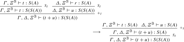 (A.2)
(A.2) -
Rules \(\Rightarrow _E\) and \(\Rightarrow _{ES}\):
 (A.3)
(A.3) -
Rules If and \(\times _I\): These rules end with a specific types not admitting two S in the head position (i.e. \({\mathbb {B}}\Rightarrow A\) and \(\varPsi \times \varPhi \)), hence removing an S or adding an S would not allow the rule to be applied, and hence, these rules followed or preceded by \(S_I\) cannot commute.


The confluence of this rewrite system is easily inferred from the fact that there are not critical pairs. The strong normalization follows from the fact that the trees are finite and all the rewrite rules push the \(S_I\) to the root of the trees.
It only remains to check that each rule preserves the semantics.
-
Rule (A.1): The following diagram gives the semantics of both trees (we only treat, without lost of generality, the case where \(A\ne S(A')\)).
Let \(h = \lambda ^{-1}\circ (\mathsf {Id}\otimes \alpha )\circ \lambda \) and \(f=Uh\). The diagram commutes by naturality of \(\eta \) with respect to f.
-
Rule (A.2): The following diagram gives the semantics of both trees (we only treat, without lost of generality, the case where \(A\ne S(A')\)).
-
1.
Definition of \(g_1\).
-
2.
\(\eta \) is a monoidal natural transformation.
-
3.
Naturality of \(\eta \) with respect to \(\hat{+}\).
-
1.
-
Rule (A.3): The following diagram gives the semantics of both trees.


-
1.
Naturality of \(\eta \) with respect to \(\varepsilon ^\varPsi \).
-
2.
\(\eta \) is a monoidal natural transformation.
\(\square \)
Lemma A.1
(Weakening) If \(\varGamma \vdash t:A\), then \(\varGamma ,\varDelta ^{\mathbb {B}}\vdash t:A\). Moreover, \(\llbracket {\varGamma ,\varDelta ^{\mathbb {B}}\vdash t:A}\rrbracket =\llbracket {\varGamma \vdash t:A}\rrbracket \circ (\mathsf {Id}\times {!})\).
Proof
It is easy to show that a tree deriving \(\varGamma \vdash t:A\) can be transformed into a tree deriving \(\varGamma ,\varDelta ^{\mathbb {B}}\vdash t:A\) just by adding \(\varDelta ^{\mathbb {B}}\) to the contexts in its axioms. Moreover, since \(FV(t)\cap \varDelta ^{\mathbb {B}}=\emptyset \), we have \(\llbracket {\varGamma ,\varDelta ^{\mathbb {B}}\vdash t:A}\rrbracket =\llbracket {\varGamma \vdash t:A}\rrbracket \circ (\mathsf {Id}\times {!})\). \(\square \)
Lemma 4.10
(Substitution) If \(\varGamma ',x:\varPsi ,\varGamma \vdash t:A\) and \(\vdash r:\varPsi \), then the following diagram commutes:

That is, \(\llbracket {\varGamma '\times \varGamma \vdash (r/x)t:A}\rrbracket =\llbracket {\varGamma ,x:\varPsi ,\varGamma '\vdash t:A}\rrbracket \circ (\mathsf {Id}\times \llbracket {\vdash r:\varPsi }\rrbracket \times \mathsf {Id})\).
Proof
By induction on the derivation of \(\varGamma ',x:\varPsi ,\varGamma \vdash t:A\). Also, we take the rules \(\alpha _I\) and \(+_I\) with \(m=1\), the generalization is straightforward.
-

-
-
 We only treat the case when \(x\in FV(t)\), the cases \(x\in FV(u)\) and \(x\in FV(u)\cap FV(t)\) are analogous.
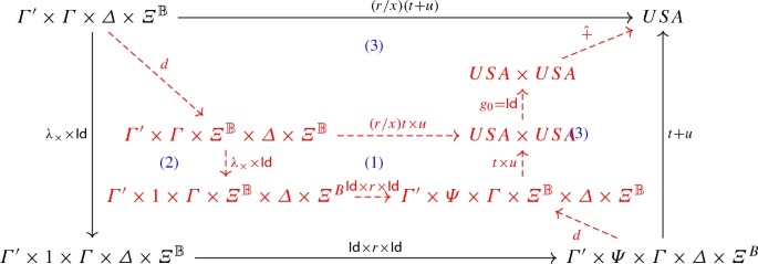
-
1.
Induction hypothesis.
-
2.
Naturality of d.
-
3.
Definition of \(+\).
-
1.
-
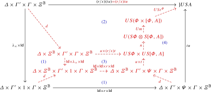
-

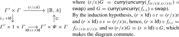
-

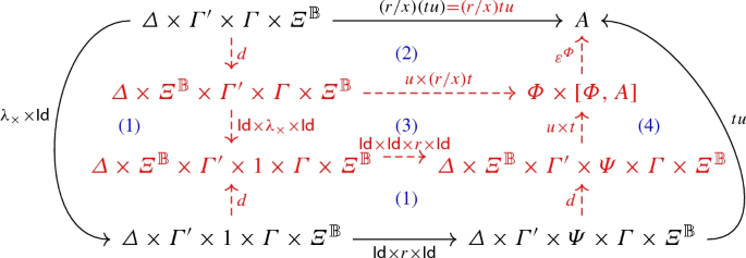
-
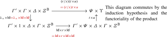
1.
Naturality of d.
-
2.
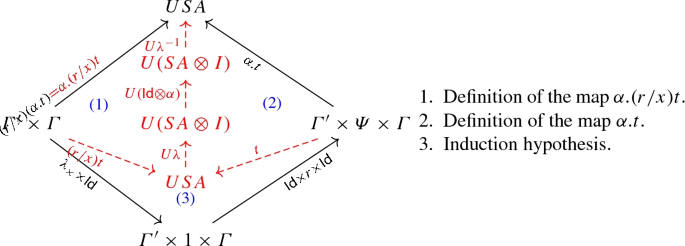
Definition of the map (r/x)tu.
-
3.
Induction hypothesis and functoriality of the product.
-
4.
Definition of the map tu.
-
1.
-
 Analogous to previous case.
 -

-
1.
Naturality of d.
-
2.
Definition of the map (r/x)tu.
-
3.
Induction hypothesis and functoriality of the product.
-
4.
Definition of the map tu.
-
1.
-
 Analogous to previous case.
 -

-
 Analogous to previous case.
 -

-

-

-
 Analogous to previous case.
 -


 We only treat the case when


 Analogous to previous case.

 Analogous to previous case.

 Analogous to previous case.


 Analogous to previous case.

\(\square \)
Theorem 4.11
(Soundness) If \(\vdash t:A\), and \(t\longrightarrow r\), then \(\llbracket {\vdash t:A}\rrbracket = \llbracket {\vdash r:A}\rrbracket \).
Proof
By induction on the rewrite relation, using the first derivable type for each term. We take the rules \(\alpha _I\) and \(+_I\) with \(m=1\), the generalization is straightforward.
- \((\mathsf {comm})\):
-
\((t+r)=(r+t)\). We have


Then,

Where \(\gamma \) is the symmetry on \(\times \) and \(\sigma \) the symmetry on \(\oplus \).
- \((\mathsf {asso})\):
-
\(((t+r)+s)=(t+(r+s))\). We have


Then

-
1.
Naturality of \(\alpha _\times \).
-
2.
Definition of \(\hat{+}\).
-
3.
U monoidal functor.
-
4.
Naturality of p with respect to \(\nabla \).
-
5.
Associativity property of \(\oplus \).
- (\(\beta _b\)):
-
If b has type \({\mathbb {B}}^n\) and \(b\in \mathsf B\), then \((\lambda x{:}{{\mathbb {B}}^n}.t)b\longrightarrow (b/x)t\). We have,


Then,

This diagram commutes because of Lemma 4.10.
- (\(\beta _n\)):
-
If u has type \(S\varPsi \), then \((\lambda x{:}{S\varPsi }.t)u\longrightarrow (u/x)t\). We have,


Then,

This diagram commutes because of Lemma 4.10.
- (\(\mathsf {If}_1\)):
-
\({|1\rangle }?{t}\mathord {\cdot }{r}\longrightarrow t\). We have,

Then,

Notice that \(\mathsf {curry}(\mathsf {uncurry}(f_{t,r})\circ \mathsf {swap})\) transforms the arrow \({\mathbb {B}}\xrightarrow {f_{t,r}}[1,A]\) (which is the arrow \(|0\rangle \mapsto r\), \(|1\rangle \mapsto t\)) into an arrow \({1}\xrightarrow {}[{\mathbb {B}},A]\), and hence, \(\varepsilon \circ (i_2\times \mathsf {curry}(\mathsf {uncurry}(f_{t,r})\circ \mathsf {swap}))=t\).
- (\(\mathsf {If}_0\)):
-
Analogous to (\(\mathsf {If}_1\)).
- (\(\mathsf {lin}_r^+\)):
-
If t has type \({\mathbb {B}}^n\Rightarrow A\), then \(t(u+v)\longrightarrow tu+tv\). We have,

and


-
1.
Definition of \(\hat{+}\).
-
2.
Naturality of \(\nabla \).
-
3.
Axiom\(_{{}_{\mathsf {Dist}}}\).
-
4.
Let \(f=\pi _1\otimes \mathsf {Id}\), \(g=\pi _2\otimes \mathsf {Id}\), and \(A=B=S{\mathbb {B}}^n\otimes [{\mathbb {B}}^n,A]\). Hence,
$$\begin{aligned} \nabla \circ \delta= & {} [\mathsf {Id},\mathsf {Id}]\circ \langle f,g\rangle \\= & {} [\mathsf {Id},\mathsf {Id}]\circ \mathsf {Id}\circ \langle f,g \rangle \\= & {} [\mathsf {Id},\mathsf {Id}]\circ (i_A\circ \pi _A+i_B\circ \pi _B)\circ \langle f,g \rangle \\= & {} (([\mathsf {Id},\mathsf {Id}]\circ i_A\circ \pi _A)+([\mathsf {Id},\mathsf {Id}]\circ i_B\circ \pi _B))\circ \langle f,g \rangle \\= & {} (\pi _A+\pi _B)\circ \langle f,g \rangle \\= & {} \pi _A\circ \langle f,g \rangle +\pi _B\circ \langle f,g \rangle \\= & {} f+g\\= & {} \pi _1\otimes \mathsf {Id}+\pi _2\otimes \mathsf {Id}\\= & {} \nabla \otimes \mathsf {Id}\end{aligned}$$ -
5.
Naturality of \(\hat{+}\).
-
6.
Naturality of \(\varDelta \).
-
7.
Definition of d.
-
8.
Naturality of \(\sigma \).
- \((\mathsf {lin}_r^ \alpha )\):
-
If t has type \({\mathbb {B}}^n\Rightarrow A\), then \(t(\alpha .u)\longrightarrow \alpha .(tu)\). We have,

Then,

-
1.
Functoriality of \(\times \).
-
2.
Naturality of n.
-
3.
Coherence of \(\sigma \).
-
4.
Naturality of \(\lambda \) with respect to m.
-
5.
Functoriality of \(\otimes \).
-
6.
Naturality of \(\lambda \) with respect to \(S\varepsilon ^{{\mathbb {B}}^n}\).
-
7.
Naturality of \(\lambda ^{-1}\) with respect to m.
- \((\mathsf {lin}^0_r)\):
-
If t has type \({\mathbb {B}}^n\Rightarrow A\), then \(t\mathbf {0}_{S({\mathbb {B}}^n)}\longrightarrow \mathbf {0}_{S(A)}\). We have,


Then,

-
1.
Naturality of \(\eta \) and functoriality of the product.
-
2.
Naturality of n.
-
3.
Property of monoidal adjunctions.
-
4.
Notice that \(\mathbf 0\otimes (St\circ m_I)=\mathbf 0\), hence, this diagram commutes by property of \(\mathbf 0\).
-
5.
Property of the morphism \(\mathbf 0\).
-
6.
Property of monoidal categories.
-
7.
Naturality of \(\lambda _\times \).
- \((\mathsf {lin}^+_l)\):
-
\((t+u)v\longrightarrow (tv+uv)\). This case is analogous to \((\mathsf {lin}^+_r)\). Notice that the axiom is valid only for \(\hat{+}\times \mathsf {Id}\), not for \(\mathsf {Id}\times \hat{+}\), however, one can be transformed into the other by using a swap.
- \((\mathsf {lin}^\alpha _l)\):
-
\((\alpha .t)u\longrightarrow \alpha .(tu)\). This case is analogous to \((\mathsf {lin}^\alpha _r)\).
- \((\mathsf {lin}^0_l)\):
-
\(\mathbf {0}_{S({\mathbb {B}}^n\Rightarrow A)}t\longrightarrow \mathbf {0}_{S(A)}\). This case is analogous to \((\mathsf {lin}^0_r)\).
- \((\mathsf {neutral})\):
-
\((\mathbf {0}_{S(A)}+t)\longrightarrow t\). We have


Then,

-
1.
By Axiom\(_{{}_0}\) and functoriality of product.
-
2.
Naturality of p.
-
3.
Definition of \(\hat{+}\).
-
4.
Naturality of \(\varDelta \).
-
5.
U preserves product.
-
6.
Property of sum in an additive category.
-
7.
The map \(\mathbf 0\) is neutral with respect to the sum.
- \((\mathsf {unit})\):
-
\(1.t\longrightarrow t\). We have


Then,

- \((\mathsf {zero}_\alpha )\):
-
If t has type A, \(0.t\longrightarrow \mathbf {0}_{S(A)}\). We have


Then,

-
1.
Axiom\(_{{}_0}\).
-
2.
Property of the map \(\mathbf 0\).
- \((\mathsf {zero})\):
-
\(\alpha .\mathbf {0}_{S(A)}\longrightarrow \mathbf {0}_{S(A)}\). We have

Then

-
1.
Same arrows.
-
2.
Property of the morphism \(\mathbf 0\).
- \((\mathsf {prod})\):
-
\(\alpha .(\beta .t)\longrightarrow (\alpha \beta ).t\). We have

Then

This diagram commutes by functoriality of \(\otimes \).
- \((\alpha \mathsf {dist})\):
-
\(\alpha .(t+u)\longrightarrow \alpha .t+\alpha .u\). We have


Then

The three subdiagrams are valid by the naturality of \(\hat{+}\).
- \((\mathsf {fact})\):
-
\((\alpha .t+\beta .t)\longrightarrow (\alpha +\beta ).t\). We have

Then

-
1.
Naturality of \(\varDelta \).
-
2.
Functor U preserves product.
-
3.
Distributivity property given by the fact that the tensor is a left adjoint.
-
4.
Naturality of \(p^{-1}\).
-
5.
Additivity of the category.
-
6.
Definition of \(\hat{+}\).
-
7.
Naturality of \(\hat{+}\).
- \((\mathsf {fact}^1)\):
-
\((\alpha .t+t)\longrightarrow (\alpha +1).t\). This case is a particular case of \(\mathsf {fact}\).
- \((\mathsf {fact}^2)\):
-
\((t+t)\longrightarrow 2.t\). This case is a particular case of \(\mathsf {fact}\).
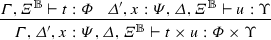
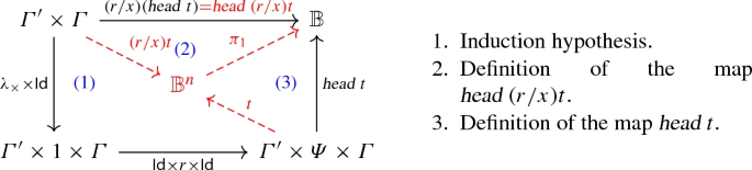
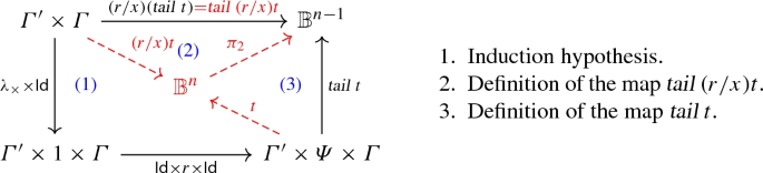
- \((\mathsf {head})\):
-
If \(h\ne u\times v\), and \(h\in \mathsf B\), \(\text { head}\ h\times t\longrightarrow h\). We have


Then

This diagram commutes since \(\pi _1\) is just the projection.
- \((\mathsf {tail})\):
-
If \(h\ne u\times v\), and \(h\in \mathsf B\), \(\text { tail}\ h\times t\longrightarrow t\). We have


Then

This diagram commutes since \(\pi _2\) is just the projection.
- (\(\mathsf {dist}_r^+\)):
-
\(\Uparrow _r ((r+s)\times u)\longrightarrow \Uparrow _r (r\times u)+\Uparrow _r (s\times u)\). We have,


Then

-
1.
Functoriality of the product.
-
2.
Naturality of \(\eta \).
-
3.
Naturality of \(\eta \) (remark that by the axioms of monads, \(\mu \circ \eta =\mathsf {Id}\)).
-
4.
Naturality of d.
-
5.
Axiom\(_{{}_{\mathsf {Dist}}}\) and definition of \(\hat{+}\).
-
6.
Naturality of \(\hat{+}\).
- (\(\mathsf {dist}_l^+\)):
-
\(\Uparrow _\ell u\times (r+s)\longrightarrow \Uparrow _\ell (u\times r)+\Uparrow _\ell (u\times s)\). Analogous to case \((\mathsf {dist}_r^+)\)
- \(({{\mathsf {dist}}^{\alpha }_{\mathsf {r}}})\):
-
\(\Uparrow _r (\alpha .r)\times u\longrightarrow \alpha .\Uparrow _r r\times u\). We have,

Then

-
1.
See next diagram.
-
2.
Naturality of \(\eta \).
-
3.
Functoriality of product.
-
4.
Naturality of n.
-
5.
Coherence.
-
6.
Naturality of \(\lambda \).

-
1.
Naturality of \(\eta \).
-
2.
Functoriality of the product.
-
3.
Naturality of n.
-
4.
Coherence
-
5.
Naturality of \(\lambda \) and functoriality of USU.
-
6.
Naturality of \(\sigma \).
-
7.
Functoriality of the tensor.
- \(({{\mathsf {dist}}^{\alpha }_{\mathsf {l}}})\):
-
\(\Uparrow _\ell u\times (\alpha .r)\longrightarrow \alpha .\Uparrow _\ell u\times r\). Analogous to case \(({{\mathsf {dist}}^{\alpha }_{\mathsf {r}}})\).
- \((\mathsf {dist}^0_{\mathsf {r}})\):
-
If u has type \(\varPhi \), \(\Uparrow _r\mathbf {0}_{S(\varPsi )}\times u\longrightarrow \mathbf {0}_{S(\varPsi \times \varPhi )}\). We have

Then

-
1.
Naturality of \(\eta \).
-
2.
Functoriality of the product.
-
3.
Naturality of \(\varDelta \).
-
4.
\(U(\mathbf{0}\otimes Su)=U\mathbf{0}\), hence, we conclude by Axiom\(_{{}_0}\) with the maps \(n\circ \varDelta \) and \(\mathsf {Id}\).
-
5.
Naturality of n.
-
6.
Property of map \(\mathbf{0}\).
- \((\mathsf {dist}^0_{\mathsf {l}})\):
-
If u has type \(\varPsi \), \(\Uparrow _\ell u\times \mathbf {0}_{S(\varPhi )}\longrightarrow \mathbf {0}_{S(\varPsi \times \varPhi )}\). Analogous to case \((\mathsf {dist}^0_{\mathsf {r}})\).
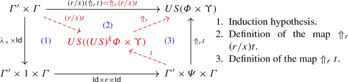
- (\(\mathsf {dist}_\Uparrow ^+\)):
-
\(\Uparrow (t+u)\longrightarrow (\Uparrow t+\Uparrow u)\). We only give the details for \(\Uparrow _r\), the case \(\Uparrow _\ell \) is analogous.


Then

This diagram commutes by naturality of \(\hat{+}\).
- (\(\mathsf {dist}_\Uparrow ^\alpha \)):
-
\(\Uparrow (\alpha .t)\longrightarrow \alpha .\Uparrow t\). We only give the details for \(\Uparrow _r\), the case \(\Uparrow _\ell \) is similar.

Then

-
1.
Naturality of \(\lambda \).
-
2.
Naturality of \(\lambda \) and the definition of monad given by an adjunction.
-
3.
Functoriality of tensor.
-
4.
Naturality of \(\lambda ^{-1}\).
-
5.
Naturality of \(\lambda ^{-1}\) and the definition of monad given by an adjunction.
- \(({\mathsf {dist}}^{\mathsf {0}}_{\Uparrow _{\mathsf {r}}})\):
-
\(\Uparrow _r\mathbf {0}_{S(S(S\varPsi )\times \varPhi )}\longrightarrow \Uparrow _r\mathbf {0}_{S(S\varPsi \times \varPhi )}\). We have


Then,

This diagram commutes by the property of the map \(\mathbf{0}\).
- \(({\mathsf {dist}}^{\mathsf {0}}_{\Uparrow _\ell })\):
-
\(\Uparrow _\ell \mathbf {0}_{S(\varPhi \times S(S\varPsi ))}\longrightarrow \Uparrow _\ell \mathbf {0}_{S(\varPhi \times S\varPsi )}\). Analogous to case \(({\mathsf {dist}}^{\mathsf {0}}_{\Uparrow _{\mathsf {r}}})\).
- \(({\mathsf {neut}}^\Uparrow _{\mathsf {r}})\):
-
If \(u\in \mathsf B\), \(\Uparrow _r u\times v\longrightarrow u\times v\). We have


Then

-
1.
Naturality of \(\eta \).
-
2.
Functoriality of product.
-
3.
Remark that \(\mu \circ US\eta = \mathsf {Id}\).
-
4.
\(\eta \) is a monoidal linear transformation.
- \(({\mathsf {neut}}^{\Uparrow }_{\ell })\):
-
If \(v\in \mathsf B\), \(\Uparrow _\ell u\times v\longrightarrow u\times v\). Analogous to case \(({\mathsf {neut}}^\Uparrow _{\mathsf {r}})\).
- \(({\mathsf {neut}}^\Uparrow _{\mathsf {0r}})\):
-
\(\Uparrow _r\mathbf {0}_{S(S({\mathbb {B}}^n)\times \varPhi )}\longrightarrow \mathbf {0}_{S({\mathbb {B}}^n\times \varPhi )}\). We have


Then,

Remark that \(\mathbf{0} = f\circ \mathbf{0}\) for any f.
- \(({\mathsf {neut}}^\Uparrow _{{\mathsf {0}}\ell })\):
-
\(\Uparrow _\ell \mathbf {0}_{S(\varPhi \times S({\mathbb {B}}^n))}\longrightarrow \mathbf {0}_{S(\varPhi \times {\mathbb {B}}^n)}\). Analogous to case \(({\mathsf {neut}}^\Uparrow _{\mathsf {0r}})\).
- Contextual rules:
-
Trivial by composition law.
\(\square \)
Lemma 4.13
(Adequacy) If \(\varGamma \vdash t:A\) and \(\sigma \vDash \varGamma \), then \(\sigma t\in , A\).
Proof
We proceed by structural induction on the derivation of \(\varGamma \vdash t:A\).
-
 Since \(\sigma \vDash \varGamma ^{\mathbb {B}},x:\varPsi \), we have \(\sigma x\in , \varPsi \).
 -
 By definition, \(\sigma \mathbf {0}_{S(A)}=\mathbf {0}_{S(A)}\in , {S(A)}\).
 -
 By definition, \(\sigma |0\rangle =|0\rangle \in , {{\mathbb {B}}}\).
 -
 By definition, \(\sigma |1\rangle =|1\rangle \in , {{\mathbb {B}}}\).
 -
By the induction hypothesis, \(\sigma t\in , {S(A)}\), hence, one of the following cases occur:
-
\(t\in \mathcal S, A\), then \(t=\sum _i\beta _ir_i\) with \(r_i\in , A\). Since \(\alpha .\sum _i\beta _ir_i\longrightarrow ^*\sum _i(\alpha \times \beta _i)r_i\), we have \(\alpha .t\in , {S(A)}\).
-
\(t\longrightarrow ^* r\) with \(r\in \mathcal S, A\), then \(t\in \overline{\mathcal S, A}\subset , {S(A)}\).
-
-
By the induction hypothesis, \(\sigma _1\sigma t,\sigma _2\sigma u\in , {S(A)}\), where \(\sigma _1\vDash \varGamma \), \(\sigma _2\vDash \varDelta \), and \(\sigma \vDash \varXi ^{\mathbb {B}}\).
By definition \(\sigma _1\sigma t+\sigma _2\sigma u=\sigma _1\sigma _2\sigma (t+u)\in , {S(A)}\).
-

By the induction hypothesis, \(\sigma t\in , A\) and \(\sigma r\in , A\). Hence, for any \(s\in , {\mathbb {B}}\), \({s}?{\sigma t}\mathord {\cdot }{\sigma r}\) reduces either to \(\sigma t\) or to \(\sigma r\), hence it is in \(, A\), therefore, \({}?{\sigma t}\mathord {\cdot }{\sigma r}\in , {{\mathbb {B}}\Rightarrow A}\).
-

Let \(r\in , \varPsi \). Then, \(\sigma (\lambda x{:}\varPsi .t)r=(\lambda x{:}\varPsi .\sigma t)r\rightarrow (r/x)\sigma t\). Since \((r/x)\sigma \vDash \varGamma ,x:\varPsi \), we have, by the induction hypothesis, that \((r/x)\sigma t\in , A\). Therefore, \(\lambda x{:}\varPsi .t\in , {\varPsi \Rightarrow A}\).
-

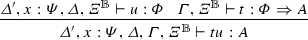
By the induction hypothesis, \(\sigma _1\sigma u\in , \varPsi \) and \(\sigma _2\sigma t\in , {\varPsi \Rightarrow A}\), where \(\sigma _1\vDash \varDelta \), \(\sigma _2\vDash \varGamma \), and \(\sigma \vDash \varXi ^{\mathbb {B}}\). Then, by definition, \(\sigma _1\sigma t\sigma _2\sigma r=\sigma _1\sigma _2\sigma (tr)\in , A\).
-

By the induction hypothesis \(\sigma _1\sigma t\in , {S(\varPsi \Rightarrow A)}=\overline{S, {\varPsi \Rightarrow A}}\) and \(\sigma _2\sigma u\in , {S\varPsi }=\overline{S, \varPsi }\), where \(\sigma _1\vDash \varGamma \), \(\sigma _2\vDash \varDelta \), and \(\sigma \vDash \varXi ^{\mathbb {B}}\).
Let \(\sigma _1\sigma t\longrightarrow ^*\sum _i\alpha _it_i\) with \(t_i\in , {\varPsi \Rightarrow A}\) and \(\sigma _2\sigma u\longrightarrow \sum _j\beta _ju_j\), with \(u_j\in , \varPsi \). Then \(\sigma _1\sigma _2\sigma (tu)=(\sigma _1\sigma t)(\sigma _2\sigma u)\longrightarrow ^*\sum _{ij}\alpha _i\beta _jt_iu_j\) with \(t_iu_j\in , A\), therefore, \(\sigma _1\sigma _2\sigma (tu)\in , {S(A)}\).
-

By the induction hypothesis, \(\sigma t\in , A\subseteq S, A\subseteq , {S(A)}\).
-
By the induction hypothesis, \(\sigma _1\sigma t\in , \varPsi \) and \(\sigma _2\sigma u\in , \varPhi \), hence, \(\sigma _1\sigma t\times \sigma _2\sigma u=\sigma _1\sigma _2\sigma (t\times u)\in , \varPsi \times , \varPhi \subseteq , {\varPsi \times \varPhi }\).
-

By the induction hypothesis, \(\sigma t\in , {{\mathbb {B}}^n}=\overline{, {\mathbb {B}}\times , {{\mathbb {B}}^{n-1}}}=\{u\mid u\longrightarrow ^*u_1\times u_2\text { with }u_1\in , {\mathbb {B}}\text { and }u_2\in , {{\mathbb {B}}^{n-1}}\}\). Hence, \(\sigma (\text { head}\ t)=\text { head}\ \sigma t\longrightarrow ^*\text { head}(u_1\times u_2)\longrightarrow u_1\in , {\mathbb {B}}\).
-

By the induction hypothesis, \(\sigma t\in , {{\mathbb {B}}^n}=\overline{, {\mathbb {B}}\times , {{\mathbb {B}}^{n-1}}}=\{u\mid u\longrightarrow ^*u_1\times u_2\text { with }u_1\in , {\mathbb {B}}\text { and }u_2\in , {{\mathbb {B}}^{n-1}}\}\). Hence, \(\sigma (\text { tail}\ t)=\text { tail}\ \sigma t\longrightarrow ^*\text { tail}(u_1\times u_2)\rightarrow u_2\in , {{\mathbb {B}}^{n-1}}\).
-

By the induction hypothesis, we have that \(\sigma t\in , {S(S\varPsi \times \varPhi )}\). Therefore, \(\sigma t\in \overline{S(\overline{\overline{S, \varPsi }\times , \varPhi })}\).
Hence, \(\sigma t\longrightarrow ^*\sum _i\alpha _i ( (\sum _{j_i}\beta _{ij_i}r_{ij_i}) \times u_i)\) with \(u_i\in , \varPhi \) and \(r_{ij_i}\in , \varPsi \).
Hence, \(\Uparrow _r t\longrightarrow ^*\sum _{j_i}(\alpha _i\beta _{ij_i})\Uparrow _r(r_{ij_i}\times u_i)\in , {S(\varPsi \times \varPhi )}\).
-
 Analogous to previous case.
 Since
Since  By definition,
  By definition,
  By definition,


 Analogous to previous case.
\(\square \)
Rights and permissions
About this article

Cite this article
Díaz-Caro, A., Malherbe, O. A Categorical Construction for the Computational Definition of Vector Spaces. Appl Categor Struct 28, 807–844 (2020). https://doi.org/10.1007/s10485-020-09598-7
Received:
Accepted:
Published:
Issue Date:
DOI: https://doi.org/10.1007/s10485-020-09598-7