

Abstract
The measurement of trace moisture is important in industry to maintain the quality and yield of products, such as semiconductors, lithium-ion batteries, and organic electroluminescence devices. In the field, on-site calibration of a trace moisture analyzer is required to maintain its reliability. Given these circumstances, we previously developed a ball surface acoustic wave (SAW) sensor using SAW on spherical piezoelectric elements and reported its quick response as its advantage over other trace moisture analyzers. However, the ultimately short response time of less than 1 s has not been verified, and it has not yet been calibrated on-site. In this study, we developed a system for the injection of saturated water vapor to evaluate the quick response of a trace moisture analyzer, and we verified the quick response time of as short as 0.64 s. It is the shortest response time reported so far. In addition, to realize its on-site calibration, we developed a dynamic calibration method, which takes only 10 min, by the injection of saturated water vapor, in contrast to the presently available static calibration method that takes 10 h. Since this system consists of simple components, it can be downsized. Moreover, because it uses a small amount of saturated water vapor as the calibration gas, it is easy to prepare calibration gases in the field and may be applied to on-site calibration.
Export citation and abstract BibTeX RIS

Original content from this work may be used under the terms of the Creative Commons Attribution 4.0 license. Any further distribution of this work must maintain attribution to the author(s) and the title of the work, journal citation and DOI.
1. Introduction
In the manufacturing of semiconductors and materials that react easily with water, such as lithium-ion batteries and organic electroluminescence, trace levels of moisture can seriously degrade device yields and performance [1–5]. Therefore, various types of trace moisture analyzer [6] are used for monitoring the trace moisture in process gases. However, they have a problem in response time, and a quick response time of less than 1 s has not been reported. In addition, on-site calibration is required to maintain the reliability of the products in the field. Generally, the calibration is performed where the sensor response to trace moisture has reached a sufficient equilibrium by maintaining the moisture concentration in the sensor cell for several hours. However, while such a static calibration method enables accurate calibration, it is difficult to apply it to on-site calibration because the calibration system is huge and the calibration takes as long as 10 h.
On the other hand, on the basis of a finding of a surface acoustic wave (SAW) that makes multiple roundtrips on spherical piezoelectric elements [7, 8], we have developed a ball SAW sensor [9–19] and applied it to a trace moisture analyzer with a sol–gel silica-based sensitive film [20–23]. Although conventional SAW sensors require a thick sensitive film to achieve high sensitivity [24], a ball SAW sensor achieves high sensitivity owing to its large propagation length realized by multiple roundtrips of the SAW, and a thin sensitive film can be employed. Since a thin sensitive film immediately equilibrates to the concentration of an ambient gas, it can respond quickly. We have reported the quick response of the ball SAW sensor as its advantage over other trace moisture analyzers [20, 21, 23]. However, its ultimately short response time of less than 1 s has not yet been verified. In addition, similarly to other trace moisture analyzers, the ball SAW trace moisture analyzer has not been calibrated on-site.
In this work, we developed a system for the injection of saturated water vapor, which enables the evaluation of the quick response of a trace moisture analyzer and on-site calibration. Using this system, we evaluated the response time of a ball SAW trace moisture analyzer and demonstrated a dynamic calibration method that can be performed in as short as 10 min and is applicable to on-site calibration.
2. Static calibration method
2.1. Static calibration system
Figure 1(a) shows a schematic diagram of the static calibration system. The calibration gas is prepared by two-step dilution of saturated water vapor generated in a saturator. The saturator is controlled at the pressure of 400 kPa and the temperature of 25 °C. First, the flow ratio between wet gas passing through the saturator and dry gas is controlled by a mass flow controller (MFC) 1 and MFC 2 to dilute the wet gas in the range of 1–200 times. Next, the diluent gas is further diluted in the range of 1–200 times by MFC 3 and MFC 4. Then, the conditioned gas is introduced into a sensor cell at a flow rate controlled by MFC 5. Here, the pressure in the sensor cell is 100 kPa. The flow rate of gas passing through MFC 3 should not be larger than total amount of gas passing through MFC 1 and MFC 2, and the excess gas is exhausted by an automatic pressure regulator (APR) 1. Similarly, the flow rate of gas passing through MFC 5 should not be larger than total amount of gas passing through MFC 3 and MFC 4, and the excess gas is exhausted by APR 2. In this way, this system can change the moisture concentration around the sensor and calibrate in the range of frost point from −87 to 4 °C.
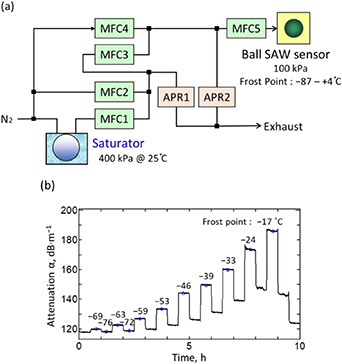
Figure 1. Static calibration method. (a) Schematic diagram of static calibration system. (b) Sensor response during static calibration.
Download figure:
Standard image High-resolution imageFigure 1(b) is an example of the ball SAW sensor response when the moisture concentration is changed stepwise using this system. This graph shows the temporal variation of the attenuation α as the response of the ball SAW sensor in 10 h when the moisture concentration evaluated as the frost point (FP) was changed in steps from −76 °C to −17 °C. From this data, a calibration curve of the relationship between the FP and the attenuation α can be obtained.
2.2. Result of static calibration
In figure 2(a), the relationships between the FP and the attenuation α of the ball SAW sensor obtained by the static calibration system are plotted as open circles. Here, we found that the relationship indicated as a dotted curve can be expressed as a function of α given by

where A, B, C, and D are coefficients, which are characteristics of each sensor. That is, the calibration of the ball SAW sensor means the determination of these coefficients. When the FP is above −25 °C, the FP can be approximated to be almost linear to α neglecting the exponential term of equation (1) as


Figure 2. Calibration curve of ball SAW sensor. (a) Relationship between attenuation of SAW (α) and frost point (FP). (b) Relationship between α and FP in the low concentration range determined using equation (3).
Download figure:
Standard image High-resolution imageTherefore, the coefficients A and B can be determined by a least squares fitting of the data in the high concentration range. Furthermore, equation (1) can be transformed to

expressing the exponential term of equation (1) as a linear function. Figure 2(b) shows the relationship between α and the values on the left-hand side of equation (3) using data in the low FP range. Therefore, the coefficients C and D can be determined by a least squares fitting. By using these coefficients, we can obtain the calibration curve for this sensor as

Furthermore, since it was found that each coefficient is almost linear to the sensor temperature near room temperature, it can be expressed by a linear function of the sensor temperature. Therefore, the coefficients for temperature compensation can be determined by fitting each coefficient from the relationship between the FP and the attenuation by changing the sensor temperature. In this paper, since the measurement was performed at a constant temperature, the explanation for the coefficient related to temperature compensation is omitted.
3. Measurement of quick response of the ball SAW trace moisture analyzer
3.1. System for evaluation of quick response and dynamic calibration
A schematic diagram of the system we developed is shown in figure 3. This system is composed of a saturated water vapor generator and a flow-controlled gas line leading to a moisture sensor. This line has an inlet to inject saturated water vapor upstream of the sensor. When the saturated water vapor is injected, the water vapor is carried to the moisture sensor by diffusion and drifting through the piping, and a sensor response is obtained, which varies with time owing to the change in moisture concentration.
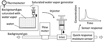
Figure 3. Schematic diagram of system for evaluation of quick response and for dynamic calibration.
Download figure:
Standard image High-resolution imageAs a saturated water vapor generator, we use a sampling gas bag for gas analysis, whose inner surface was inactivated, as shown in figure 4(a). The size of the gas bag is 1 l. After purging the gas bag with nitrogen gas, pure water is injected into the bag and the bag is saturated with water vapor at room temperature controlled by an air conditioner. As an injector, we use a gas-tight syringe, with which we can control the injection volume using its scale. The saturated water vapor is extracted from the gas bag and injected into the inlet provided 170 mm upstream of the ball SAW sensor connected to the nitrogen pipe by manual operation of the gas-tight syringe. The dry nitrogen gas line is shown in figure 4(b). The sensor is in a small cell whose volume is 1.4 ml. The nitrogen gas flow is controlled using a mass flow controller. This injection is used both for the evaluation of response time and for a dynamic calibration, which will be described in section 4.

Figure 4. Dynamic calibration system. (a) Gas bag for saturated water vapor generator and gas-tight syringe as the injector. (b) Dry nitrogen gas line.
Download figure:
Standard image High-resolution image3.2. Evaluation of response time
We installed a ball SAW sensor into the system we developed and measured the attenuation by injecting saturated water vapor. The injection volume was 1 ml and the flow rate of the background gas was 100 ml min−1. At this time, the room temperature was 21.6 °C. Response time was evaluated as the time within which a 10%–90% increase in the FP was observed after the injection of saturated water vapor.
Figure 5(a) shows a temporal variation of the FP due to the injection of saturated water vapor measured using the ball SAW sensor. The FP increased immediately after injection and then decreased gradually. The decrease took about 10 min and is considered to represent a process at which the water adsorbed on the pipe surface was gradually desorbed. The expanded view of the peak is shown in figure 5(b). The response time taken for 10%–90% of the FP change from −70 °C to 10 °C was only 0.64 s. It is considered to be the shortest response time of the trace moisture analyzer reported so far.

Figure 5. Quick response of ball SAW trace moisture analyzer. (a) Temporal variation of FP measured by ball SAW trace moisture analyzer. (b) Expanded view of peak. (c) Video (supplemental data stacks.iop.org/MST/31/094003/mmedia).
Download figure:
Standard image High-resolution imageFurthermore, since the response time is less than 1 s, it can be regarded that the equilibrium between the water concentration within the sensitive film and that in the atmosphere is rapidly reached at any instance of the dynamic calibration process, which takes 10 min. This rapid equilibrium is the basis for the validity of the dynamic calibration process.
4. Dynamic calibration method
4.1. Procedure of dynamic calibration
First, to obtain a reference data for dynamic calibration, we install a ball SAW sensor calibrated by the static method described in section 2 into the developed system and measure the temporal variation of the attenuation by the injection of saturated water vapor. The temporal variation of the FP can be obtained by substituting the attenuation α at each time in equation (4).
Next, the ball SAW sensor is replaced with a new sensor to be calibrated, and the temporal variation of the attenuation α is measured for 10 min under the same conditions as when the reference data was measured. The calibration curve of this sensor is derived as the relationship between the attenuation α and the FP of the reference data at the same time. Finally, the sensor is calibrated again by the static method and the calibration curve obtained is compared with that obtained by the dynamic calibration method.
4.2. Measurement result of dynamic calibration
The measurement result for the reference data is shown in figure 6 at a background gas flow rate of 10 ml min−1, a saturated water vapor injection volume of 1 ml, and a room temperature of 21 °C. From the temporal variation of the attenuation α after the injection of saturated water vapor, as shown in figure 6(a), that of FP was obtained using the calibration curve obtained using equation (4), as shown in figure 6(b). Since the rising part of the peak changes rapidly, it is not used for the calibration, and the gradually decreasing part of the curve shown in red is used as reference data.

Figure 6. Reference data for dynamic calibration. (a) Temporal variation of attenuation of SAW after injection of saturated water vapor and (b) the relationship between FP and time calculated using equation (4).
Download figure:
Standard image High-resolution imageThe attenuation α of a new sensor under the same condition as the measurement for the reference data is shown by the black curve in figure 7(a). Using the reference data shown by the red curve at the same time, we obtained the FP at the right axis. Figure 7(b) shows the relationship between the attenuation α and the FP in the high concentration range as shown by closed circles. Since this relationship is almost linear, the coefficients of calibration curves A and B were determined to be A = 1.188 and B = −94.41 by a least squares fitting. On the other hand, figure 7(c) shows the relationship between the attenuation α and the function on the left-hand side of equation (3) in the low concentration range as shown by open circles. Since this relationship is also linear, coefficients C and D were determined to be C = −0.1983 and D = 11.88 by a least squares fitting. Therefore, the calibration curve of this sensor obtained by the dynamic calibration method is given by


Figure 7. Procedure of dynamic calibration. (a) Reference data and response of new sensor. (b) Relationship between attenuation and frost point in high concentration range. (c) Relationship between attenuation and left-hand-side of equation (3) in low concentration range.
Download figure:
Standard image High-resolution imageOn the other hand, the calibration curve of the same sensor obtained by the static calibration method is given by

In figure 8, the result of dynamic calibration curve using equation (5) is shown as a solid curve and that of the static calibration curve using equation (6) is shown as a dotted curve. These two curves look nearly identical.
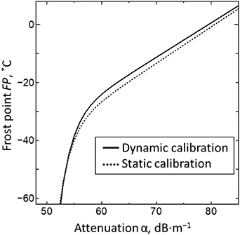
Figure 8. Calibration curves obtained by dynamic calibration and static calibration.
Download figure:
Standard image High-resolution image5. Discussion
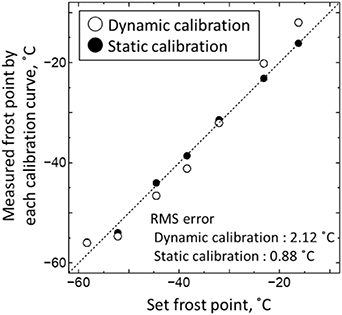
We evaluated the measurement error of FP obtained by the static and dynamic calibration methods. Figure 9 shows the error between the set FP and the measured FP calculated by the substitution of the attenuation α into each calibration curve. The horizontal axis shows the set FP and the vertical axis shows the measured FP. If there is no error, the measured FP should be plotted on the 45° line shown by the dotted line. Closed circles show results obtained by the dynamic calibration and open circles show those obtained by the static calibration. In the FP range from −59 °C to −17 °C, the RMS errors of the static and dynamic calibration methods were 0.88 °C and 2.12 °C, respectively.
Figure 9. Relationship between set FP and measured FP determined using each calibration curve.
Download figure:
Standard image High-resolution image
The RMS error of 2.12 °C of the dynamic calibration in the FP range from −59 °C to −17 °C may not be small for accurate calibration. However, the dynamic calibration will be useful for a rough estimate of the sensor condition in the field checking whether the sensor response has changed significantly. Since this error is considered to be the accumulation of errors in the calibration curve obtained using equation (4) acquired as the reference data, errors in the amount of injected saturated water vapor as the calibration gas, and subtle differences in temperature and atmospheric pressure, it can be reduced by improving the system components.
In this study, we used dry nitrogen as a background gas for the dynamic calibration system. However, when calibrating a sensor used in an environment other than nitrogen, it is necessary to use the same type of dry gas as that environment. Also, the reference data used for the dynamic calibration must be obtained under the same background gas. This is because the diffusion of the injected saturated water vapor changes depending on the background gas.
The dynamic calibration system developed in this study has a significant advantage of having a measurement time as short as 10 min, in contrast to the 10 h measurement time of the static calibration [22]. Since it consists of simple components, it is possible to downsize the calibration system and apply it to on-site calibration. In addition, since it uses a small amount of saturated water vapor as the calibration gas, it is easy to prepare calibration gases in the field and may be applied to special gases for which calibration gases are not easy to obtain in large amounts. Furthermore, this system can be applied to not only ball SAW sensors, but also the calibration of trace moisture analyzers with a quick response.
6. Conclusion
We developed a system and method for the evaluation of the quick response of a trace moisture analyzer and for dynamic calibration using saturated water vapor. We installed a ball SAW sensor in this system and measured the temporal variation of the attenuation after the injection of saturated water vapor. The 10%–90% response time for the FP change from −70 °C to 10 °C was only 0.64 s when the flow rate of the background gas was 100 ml min−1. It is the shortest response time of a trace moisture analyzer reported so far. On the basis of this quick response enabling the rapid equilibrium of water concentration, the dynamic calibration of the ball SAW sensor was performed using this system. In a 10 min measurement, which is much shorter than the 10 h of the static calibration, we succeeded in calibrating the sensor with the RMS error of 2.12 °C in the FP range of −59 °C to −17 °C. Therefore, this system can be applied to the on-site calibration of a trace moisture analyzer in the field.
Supplementary Material
Supplementary material for this article is available online