


1 Introduction
The electromotive force (EMF)  $\boldsymbol{u}\times \boldsymbol{B}$ as the vector product of flow velocity and magnetic field is the only nonlinear term in the induction equation on which the present-day mean-field electrodynamics is based on. It is the only nonlinear term in this equation if the microscopic magnetic diffusivity
  $\unicode[STIX]{x1D702}$ in the fluid is uniform. This, however, is not necessarily true. If for any reason the electric conductivity fluctuates around a certain average value then the local diffusivity fluctuates around its basal value so that the effective decay time of a large-scale electric current is changed. Below, we shall demonstrate this phenomenon – which reduces the effective eddy diffusivity of a turbulence field (Krause & Roberts Reference Krause and Roberts1973) – also with nonlinear simulations.
In convection-driven turbulent fields temperature fluctuations should produce electric-conductivity fluctuations which are correlated with the vertical component of the flow field. In this case, even a turbulent diffusivity flux vector  $\langle \unicode[STIX]{x1D702}^{\prime }\boldsymbol{u}^{\prime }\rangle$ occurs which in connection with the large-scale field and/or the large-scale electric current may form new terms in the mean-field induction equation. Pétrélis, Alexakis & Gissinger (Reference Pétrélis, Alexakis and Gissinger2016) assumed that a new sort of alpha effect arises in such systems. Our considerations confirm the existence of an alpha effect but only in the presence of global rotation. Without rotation the conductivity fluctuations will (only) lead to a reduction of the eddy diffusivity and – if correlated with one of the velocity components – to a new diamagnetic pumping term.
2 The equations
The problem is mainly described by the induction equation
 $$\begin{eqnarray}\displaystyle \frac{\unicode[STIX]{x2202}\boldsymbol{B}}{\unicode[STIX]{x2202}t}=\text{curl}(\boldsymbol{u}\times \boldsymbol{B}-\unicode[STIX]{x1D702}\,\text{curl}\,\boldsymbol{B}), & & \displaystyle\end{eqnarray}$$
 with  $\text{div}\,\boldsymbol{B}=0$ and
  $\text{div}\,\boldsymbol{u}=0$ for an incompressible fluid. Here
  $\boldsymbol{u}$ is the velocity,
  $\boldsymbol{B}$ is the magnetic field vector and
  $\unicode[STIX]{x1D702}$ the magnetic diffusivity. We consider a turbulent fluid with
  $\boldsymbol{u}=\bar{\boldsymbol{u}}+\boldsymbol{u}^{\prime }$ and with a fluctuating magnetic diffusivity
  $\unicode[STIX]{x1D702}=\bar{\unicode[STIX]{x1D702}}+\unicode[STIX]{x1D702}^{\prime }$. For the expectation values of the perturbations we shall use the notations
  $u_{\text{rms}}=\langle {\boldsymbol{u}^{\prime }}^{2}\rangle ^{1/2}$ and
  $\unicode[STIX]{x1D702}_{\text{rms}}=\langle {\unicode[STIX]{x1D702}^{\prime }}^{2}\rangle ^{1/2}$. Large-scale observables (mean values) are marked with overbars while brackets are used for the correlations of fluctuations. For finite fluctuations the high-conductivity limit
  $\bar{\unicode[STIX]{x1D702}}\rightarrow 0$ is not allowed. The fluctuations
  $\boldsymbol{u}^{\prime }$ and
  $\unicode[STIX]{x1D702}^{\prime }$ may be correlated so that a turbulence-originated diffusivity flux
 $$\begin{eqnarray}\boldsymbol{U}=\langle \unicode[STIX]{x1D702}^{\prime }\boldsymbol{u}^{\prime }\rangle\end{eqnarray}$$
 forms a vector which is polar by definition. The existence of this vector is obvious for thermal convection, when both the velocity field and the electric conductivity are due to temperature fluctuations. The correlation (2.2) can be understood as the transport of magnetic diffusivity in a preferred direction. Also the magnetic field will fluctuate, i.e.  $\boldsymbol{B}=\bar{\boldsymbol{B}}+\boldsymbol{B}^{\prime }$. The magnetic fluctuation
  $\boldsymbol{B}^{\prime }$ fulfils a nonlinear induction equation which follows from (2.1). We shall only discuss its linear version
 $$\begin{eqnarray}\displaystyle \frac{\unicode[STIX]{x2202}\boldsymbol{B}^{\prime }}{\unicode[STIX]{x2202}t}=\text{curl}(\boldsymbol{u}^{\prime }\times \bar{\boldsymbol{B}}-\bar{\unicode[STIX]{x1D702}}\,\text{curl}\,\boldsymbol{B}^{\prime }-\unicode[STIX]{x1D702}^{\prime }\,\text{curl}\,\bar{\boldsymbol{B}}) & & \displaystyle\end{eqnarray}$$
in the analytical theory of driven turbulence (Krause & Rädler Reference Krause and Rädler1980). The results of the calculations within the quasilinear first-order smoothing approximation will also be probed by targeted numerical simulations with well-established nonlinear codes.
If the fluctuations are known in their dependences on the magnetic background field and rotation then the turbulence-originated EMF  $\boldsymbol{{\mathcal{E}}}=\langle \boldsymbol{u}^{\prime }\times \boldsymbol{B}^{\prime }\rangle$ and the diffusivity–current correlation
 $$\begin{eqnarray}\boldsymbol{{\mathcal{J}}}=-\langle \unicode[STIX]{x1D702}^{\prime }\text{curl}\,\boldsymbol{B}^{\prime }\rangle\end{eqnarray}$$
can be formed which enter the induction equation for the large-scale field via
 $$\begin{eqnarray}\frac{\unicode[STIX]{x2202}\bar{\boldsymbol{B}}}{\unicode[STIX]{x2202}t}=\text{curl}(\boldsymbol{{\mathcal{E}}}+\boldsymbol{{\mathcal{J}}}-\bar{\unicode[STIX]{x1D702}}\,\text{curl}\,\bar{\boldsymbol{B}}).\end{eqnarray}$$
 To find the influence of a large-scale field and/or its gradients on the EMF  $\boldsymbol{{\mathcal{E}}}$ at linear order it is enough to solve the induction equation (2.3) where the inhomogeneous large-scale magnetic field may be written in the form
  $\bar{B}_{j}=B_{jp}x_{p}$ with
  $B_{jp}\equiv \bar{B}_{j,p}$. Without any loss of generality, the coordinate
  $\boldsymbol{x}=0$ defines the point where the background field vanishes. We also note that the global rotation here only appears in the Navier–Stokes equation for the velocity fluctuation which remains homogeneous if only expressions linear in
  $B_{jp}$ are envisaged. One can thus work with
 $$\begin{eqnarray}\left.\begin{array}{@{}c@{}}\displaystyle u_{i}^{\prime }(\boldsymbol{x},t)=\iint \hat{u} _{i}(\boldsymbol{k},\unicode[STIX]{x1D714})\text{e}^{\text{i}(\boldsymbol{k}\boldsymbol{x}-\unicode[STIX]{x1D714}t)}\,\text{d}\boldsymbol{k}\,\text{d}\unicode[STIX]{x1D714},\\ \displaystyle B_{i}^{\prime }(\boldsymbol{x},t)=\iint (\hat{B}_{i}(\boldsymbol{k},\unicode[STIX]{x1D714})+x_{l}\hat{B}_{il}(\boldsymbol{k},\unicode[STIX]{x1D714}))\text{e}^{\text{i}(\boldsymbol{k}\boldsymbol{x}-\unicode[STIX]{x1D714}t)}\,\text{d}\boldsymbol{k}\,\text{d}\unicode[STIX]{x1D714}.\end{array}\right\}\end{eqnarray}$$
The result is
 $$\begin{eqnarray}\hat{B}_{i}=\frac{\text{i}x_{l}k_{j}B_{jl}}{-\text{i}\unicode[STIX]{x1D714}+\bar{\unicode[STIX]{x1D702}}k^{2}}\hat{u} _{i}-\frac{B_{ij}+{\displaystyle \frac{2\bar{\unicode[STIX]{x1D702}}k_{l}k_{m}B_{lm}\unicode[STIX]{x1D6FF}_{ij}}{-\text{i}\unicode[STIX]{x1D714}+\bar{\unicode[STIX]{x1D702}}k^{2}}}}{-\text{i}\unicode[STIX]{x1D714}+\bar{\unicode[STIX]{x1D702}}k^{2}}\hat{u} _{j}+\frac{\text{i}k_{j}(B_{ij}-B_{ji})}{-\text{i}\unicode[STIX]{x1D714}+\bar{\unicode[STIX]{x1D702}}k^{2}}\hat{\unicode[STIX]{x1D702}}\end{eqnarray}$$
 as the spectral component of the magnetic fluctuations (Rüdiger, Kitchatinov & Hollerbach Reference Rüdiger, Kitchatinov and Hollerbach2013). The first two terms on the right-hand side of this equation describe the interaction of the turbulence with the large-scale magnetic field and its gradients. Under the assumption that the large-scale field  $\bar{\boldsymbol{B}}$ varies slowly in space and time, the electromotive force can be written as
 $$\begin{eqnarray}\displaystyle \boldsymbol{{\mathcal{E}}}=\unicode[STIX]{x1D6FC}\circ \bar{\boldsymbol{B}}-\unicode[STIX]{x1D702}_{\text{t}}\,\text{curl}\,\bar{\boldsymbol{B}}, & & \displaystyle\end{eqnarray}$$
 where the tensor  $\unicode[STIX]{x1D6FC}$ and the coefficient
  $\unicode[STIX]{x1D702}_{\text{t}}$ represent the
  $\unicode[STIX]{x1D6FC}$ effect and the turbulent magnetic diffusivity.
The last term in (2.7) directs the influence of the fluctuating diffusivity. It leads to an EMF of
 $$\begin{eqnarray}{\mathcal{E}}_{i}=\unicode[STIX]{x1D716}_{iqp}\iint \frac{\text{i}k_{j}\hat{U} _{q}}{-\text{i}\unicode[STIX]{x1D714}+\bar{\unicode[STIX]{x1D702}}k^{2}}\,\text{d}\boldsymbol{k}\,\text{d}\unicode[STIX]{x1D714}(B_{pj}-B_{jp}),\end{eqnarray}$$
 where  $\hat{\boldsymbol{U}}$ is the Fourier transform of the diffusivity–velocity correlation
  $\boldsymbol{U}$ which itself is a polar vector. The spectral vector of the correlation (2.2) can in full generality be written as
 $$\begin{eqnarray}\hat{U} _{i}=u_{1}\left[g_{i}-\frac{(\boldsymbol{g}\boldsymbol{k})k_{i}}{k^{2}}\right]+u_{2}\text{i}\unicode[STIX]{x1D716}_{ijk}k_{j}g_{k}.\end{eqnarray}$$
 The vector  $\boldsymbol{g}$ gives the unit vector of the coordinate in which direction the correlation between velocity and diffusivity is non-vanishing. The expression (2.10) must be odd in
  $\boldsymbol{g}$ and the real part must be even in the wavenumber
  $\boldsymbol{k}$. The quantity
  $u_{1}$ reflects the correlation of the velocity component
  $\boldsymbol{g}\boldsymbol{u}^{\prime }$ with
  $\unicode[STIX]{x1D702}^{\prime }$. The second term in (2.10) contains a correlation of diffusivity and vorticity where
  $u_{2}$ must be a pseudoscalar. Equations (2.9) and (2.10) lead to
 $$\begin{eqnarray}\boldsymbol{{\mathcal{E}}}=\iint \frac{\bar{\unicode[STIX]{x1D702}}k^{4}u_{2}}{\unicode[STIX]{x1D714}^{2}+\bar{\unicode[STIX]{x1D702}}^{2}k^{4}}\,\text{d}\boldsymbol{k}\,\text{d}\unicode[STIX]{x1D714}\quad \boldsymbol{g}\times \bar{\boldsymbol{J}},\end{eqnarray}$$
 with  $\bar{\boldsymbol{J}}=\text{curl}\,\bar{\boldsymbol{B}}$ and
  $(\boldsymbol{g}\times \bar{\boldsymbol{J}})_{i}=-(\boldsymbol{g}\boldsymbol{\cdot }\unicode[STIX]{x1D735})\bar{B}_{i}+\unicode[STIX]{x1D735}_{i}\ldots$, where the latter symbol represents a gradient which does not play a role in the induction equation. We note that the non-potential term only exists if the magnetic field
  $\bar{\boldsymbol{B}}$ depends on the coordinate along
  $\boldsymbol{g}$.
2.1 The diffusivity–current correlation
The diffusivity–current correlation  $\boldsymbol{{\mathcal{J}}}$ from (2.4) is now analysed in detail. Fourier transformed fluctuations of the electric current are
 $$\begin{eqnarray}\text{curl}_{i}\,\hat{\boldsymbol{B}}=-\frac{\unicode[STIX]{x1D716}_{isp}k_{j}k_{s}}{-\text{i}\unicode[STIX]{x1D714}+\bar{\unicode[STIX]{x1D702}}k^{2}}(\hat{u} _{p}B_{j}+\hat{\unicode[STIX]{x1D702}}(B_{pj}-B_{jp})).\end{eqnarray}$$
 Multiplication with the (negative) Fourier transform of the diffusivity fluctuation,  $\hat{\unicode[STIX]{x1D702}}$, leads to
 $$\begin{eqnarray}\hat{{\mathcal{J}}}_{i}=\frac{\unicode[STIX]{x1D716}_{isp}k_{j}k_{s}}{-\text{i}\unicode[STIX]{x1D714}+\bar{\unicode[STIX]{x1D702}}k^{2}}(\hat{U} _{p}B_{j}+\hat{V}(B_{pj}-B_{jp})).\end{eqnarray}$$
 Here,  $\hat{V}$ is here the spectral function of the autocorrelation function
  $V=\langle \unicode[STIX]{x1D702}^{\prime }(\boldsymbol{x},t)\unicode[STIX]{x1D702}^{\prime }(\boldsymbol{x}+\unicode[STIX]{x1D743},t+\unicode[STIX]{x1D70F})\rangle$ of the diffusivity fluctuations. Equations (2.10) and (2.13) provide
  $\boldsymbol{{\mathcal{J}}}=-\unicode[STIX]{x1D6FE}\boldsymbol{g}\times \bar{\boldsymbol{B}}$ with
 $$\begin{eqnarray}\unicode[STIX]{x1D6FE}=\frac{1}{3}\iint \frac{\bar{\unicode[STIX]{x1D702}}k^{4}u_{1}}{\unicode[STIX]{x1D714}^{2}+\bar{\unicode[STIX]{x1D702}}^{2}k^{4}}\,\text{d}\boldsymbol{k}\,\text{d}\unicode[STIX]{x1D714},\end{eqnarray}$$
 representing a turbulent transport of the magnetic background field (‘pumping’) anti-parallel to  $\boldsymbol{g}$. For positive
  $u_{1}$ (i.e. for positive correlation of
  $\unicode[STIX]{x1D702}^{\prime }$ and
  $u_{z}^{\prime }$) the pumping goes downwards as
  $\boldsymbol{g}$ is the vertical unit vector. We note that formally the integral in (2.14) also exists in the high-conductivity limit
  $\bar{\unicode[STIX]{x1D702}}\rightarrow 0$ so that for small
  $\bar{\unicode[STIX]{x1D702}}$ it does not depend on the magnetic Reynolds number
 $$\begin{eqnarray}Rm=\frac{u_{\text{rms}}\ell }{\bar{\unicode[STIX]{x1D702}}},\end{eqnarray}$$
 (with  $\ell$ as the correlation length) for large
  $Rm$. In this limit
  $\unicode[STIX]{x1D6FE}$ is linear in the correlation function
  $u_{1}$. For small
  $Rm$ the integral in (2.14) linearly grows with
  $Rm$, which follows after application of the extremely steep correlation function
  $\unicode[STIX]{x1D6FF}(\unicode[STIX]{x1D714})$ as a proxy of the low-conductivity limit.
On the other hand, the term with  $\hat{V}$ in (2.13) leads to
 $$\begin{eqnarray}\boldsymbol{{\mathcal{J}}}=\cdots +\frac{2}{3}\iint \frac{k^{2}\hat{V}}{-\text{i}\unicode[STIX]{x1D714}+\bar{\unicode[STIX]{x1D702}}k^{2}}\,\text{d}\boldsymbol{k}\,\text{d}\unicode[STIX]{x1D714}\,\text{curl}\,\bar{\boldsymbol{B}},\end{eqnarray}$$
 which provides an extra contribution to the magnetic field dissipation. The question is whether this term reduces or enhances the eddy diffusivity  $\unicode[STIX]{x1D702}_{\text{t}}$ which is due to the turbulence without
  $\unicode[STIX]{x1D702}$-fluctuations. For homogeneous turbulence one finds from (2.7)
 $$\begin{eqnarray}{\mathcal{E}}_{i}=-\unicode[STIX]{x1D716}_{ijp}\iint \left(B_{pn}\hat{Q}_{jn}+\frac{2\bar{\unicode[STIX]{x1D702}}k_{l}k_{m}}{-\text{i}\unicode[STIX]{x1D714}+\bar{\unicode[STIX]{x1D702}}k^{2}}B_{lm}\hat{Q}_{jp}\right)\frac{\text{d}\,\boldsymbol{k}\,\text{d}\unicode[STIX]{x1D714}}{-\text{i}\unicode[STIX]{x1D714}+\bar{\unicode[STIX]{x1D702}}k^{2}}.\end{eqnarray}$$
 The spectral tensor  $\hat{Q}_{ij}$ for isotropic turbulence is
 $$\begin{eqnarray}\hat{Q}_{ij}(\boldsymbol{k},\unicode[STIX]{x1D714})=\frac{E(k,\unicode[STIX]{x1D714})}{16\unicode[STIX]{x03C0}k^{2}}\left(\unicode[STIX]{x1D6FF}_{ij}-\frac{k_{i}k_{j}}{k^{2}}\right)-\text{i}\unicode[STIX]{x1D716}_{ijk}k_{k}H(k,\unicode[STIX]{x1D714}),\end{eqnarray}$$
 where the positive–definite spectrum  $E$ gives the energy
 $$\begin{eqnarray}u_{\text{rms}}^{2}=\int _{0}^{\infty }\int _{0}^{\infty }E(k,\unicode[STIX]{x1D714})\,\text{d}k\,\text{d}\unicode[STIX]{x1D714}\end{eqnarray}$$
 and  $H$ is the helical part of the turbulence field. From (2.17) follows
  $\boldsymbol{{\mathcal{E}}}=-\unicode[STIX]{x1D702}_{\text{t}}\,\text{curl}\,\bar{\boldsymbol{B}}$ with the positive eddy diffusivity
 $$\begin{eqnarray}\unicode[STIX]{x1D702}_{\text{t}}=\frac{1}{24\unicode[STIX]{x03C0}}\iint \frac{\bar{\unicode[STIX]{x1D702}}E}{\unicode[STIX]{x1D714}^{2}+\bar{\unicode[STIX]{x1D702}}^{2}k^{4}}\,\text{d}\boldsymbol{k}\,\text{d}\unicode[STIX]{x1D714}.\end{eqnarray}$$
For the sum of the turbulence-originated terms in (2.5) one obtains
 $$\begin{eqnarray}\displaystyle \boldsymbol{{\mathcal{E}}}+\boldsymbol{{\mathcal{J}}} & = & \displaystyle -\left(\frac{1}{24\unicode[STIX]{x03C0}}\iint \frac{\bar{\unicode[STIX]{x1D702}}E}{\unicode[STIX]{x1D714}^{2}+\bar{\unicode[STIX]{x1D702}}^{2}k^{4}}\,\text{d}\boldsymbol{k}\,\text{d}\unicode[STIX]{x1D714}-\frac{2}{3}\iint \frac{\bar{\unicode[STIX]{x1D702}}k^{4}\hat{V}}{\unicode[STIX]{x1D714}^{2}+\bar{\unicode[STIX]{x1D702}}^{2}k^{4}}\,\text{d}\boldsymbol{k}\,\text{d}\unicode[STIX]{x1D714}\right)\text{curl}\,\bar{\boldsymbol{B}}\nonumber\\ \displaystyle & & \displaystyle -\,\frac{1}{3}\iint \frac{\bar{\unicode[STIX]{x1D702}}k^{4}u_{1}}{\unicode[STIX]{x1D714}^{2}+\bar{\unicode[STIX]{x1D702}}^{2}k^{4}}\,\text{d}\boldsymbol{k}\,\text{d}\unicode[STIX]{x1D714}\quad \boldsymbol{g}\times \bar{\boldsymbol{B}},\end{eqnarray}$$
 indicating the total turbulent diffusivity as reduced by the conductivity fluctuations. On the other hand, the pumping term in the second line of this equations only exists if these conductivity fluctuations are correlated with the flow component in a preferred direction within the fluid. All terms in (2.21) also exist in the high-conductivity limit,  $\bar{\unicode[STIX]{x1D702}}\rightarrow 0$.
The modified eddy diffusivity is
 $$\begin{eqnarray}\displaystyle \frac{\unicode[STIX]{x1D702}_{\text{t}}^{\text{eff}}}{\bar{\unicode[STIX]{x1D702}}}=\frac{1}{24\unicode[STIX]{x03C0}}\iint \frac{E}{\unicode[STIX]{x1D714}^{2}+\bar{\unicode[STIX]{x1D702}}^{2}k^{4}}\,\text{d}\boldsymbol{k}\,\text{d}\unicode[STIX]{x1D714}-\frac{2}{3}\iint \frac{k^{4}\hat{V}}{\unicode[STIX]{x1D714}^{2}+\bar{\unicode[STIX]{x1D702}}^{2}k^{4}}\,\text{d}\boldsymbol{k}\,\text{d}\unicode[STIX]{x1D714} & & \displaystyle\end{eqnarray}$$
 (see Krause & Roberts Reference Krause and Roberts1973). For large  $Rm$ both terms grow linearly with
  $Rm$ while for small
  $Rm$ both terms formally grow with
  $Rm^{2}$. If the second expression is considered a function of
  $\unicode[STIX]{x1D702}_{\text{rms}}/\bar{\unicode[STIX]{x1D702}}$ then it runs with
  $1/Rm$ for large
  $Rm$ and with
  $Rm^{0}$ for small
  $Rm$. As it should, the reduction of the eddy diffusivity by conductivity fluctuations disappears in the high-conductivity limit.
Discussing possible dynamo effects in hot Jupiter atmospheres, Rogers & McElwaine (Reference Rogers and McElwaine2017) considered variable molecular diffusivities which form patterns in the vertical direction and the horizontal plane. In the horizontal plane the quasi-two-dimensional velocity field existed without being correlated with the diffusivity. In consequence, the effective magnetic diffusivity is also reduced as in (2.22) but the pumping term (2.14) does not appear.
2.2 Direct numerical simulations
To test theoretical predictions, we run fully nonlinear numerical simulations with the Pencil CodeFootnote 1. We solved the equations of compressible magnetohydrodynamics
 $$\begin{eqnarray}\displaystyle & \displaystyle \frac{\unicode[STIX]{x2202}\boldsymbol{A}}{\unicode[STIX]{x2202}t}=\boldsymbol{u}\times \boldsymbol{B}-(\bar{\unicode[STIX]{x1D702}}+\unicode[STIX]{x1D702}^{\prime })\unicode[STIX]{x1D707}_{0}\,\boldsymbol{J}+\boldsymbol{{\mathcal{E}}}_{0}, & \displaystyle\end{eqnarray}$$
 $$\begin{eqnarray}\displaystyle & \displaystyle \frac{\text{D}\ln \unicode[STIX]{x1D70C}}{\text{D}t}=-\text{div}\,\boldsymbol{u},\quad \frac{\text{D}\boldsymbol{u}}{\text{D}t}=-c_{\text{s}}^{2}\ln \unicode[STIX]{x1D70C}+\boldsymbol{F}^{\text{visc}}+\boldsymbol{F}^{\text{force}}, & \displaystyle\end{eqnarray}$$
 where  $\boldsymbol{A}$ is the magnetic vector potential and
  $\boldsymbol{B}=\text{curl}\,\boldsymbol{A}$ is the magnetic field,
  $\boldsymbol{J}=\unicode[STIX]{x1D707}_{0}^{-1}\text{curl}\,\boldsymbol{B}$ is the current density,
  $\text{D}/\text{D}t=\unicode[STIX]{x2202}/\unicode[STIX]{x2202}t+\boldsymbol{u}\boldsymbol{\cdot }\unicode[STIX]{x1D735}$ is the advective time derivative,
  $\unicode[STIX]{x1D70C}$ is the density and
  $c_{\text{s}}$ is the constant speed of sound. The last term of (2.23) describes an imposed EMF
  $\boldsymbol{{\mathcal{E}}}_{0}=\hat{{\mathcal{E}}}_{0}\sin (k_{1}x)\hat{\boldsymbol{e}}_{z}$, that is used to introduce a large-scale magnetic field
  $\bar{B}_{y}(x)$ to the system. Furthermore, the fluctuating component of the magnetic diffusivity is given by
  $\unicode[STIX]{x1D702}^{\prime }=c_{u}u_{z}$, where
  $c_{u}$ is used to control the strength of the correlation. We use
  $\unicode[STIX]{x1D702}_{\text{rms}}=c_{u}u_{z,\text{rms}}$ to quantify the amplitude of the fluctuating part of the diffusivity.
The viscous force is given by the standard expression
 $$\begin{eqnarray}\displaystyle \boldsymbol{F}^{\text{visc}}=\unicode[STIX]{x1D708}\left(\unicode[STIX]{x1D6FB}^{2}\boldsymbol{u}+{\textstyle \frac{1}{3}}\unicode[STIX]{x1D735}\unicode[STIX]{x1D735}\boldsymbol{\cdot }\boldsymbol{u}\right), & & \displaystyle\end{eqnarray}$$
 where  $\unicode[STIX]{x1D708}$ is the kinematic viscosity. The fluid is forced with an external body force
  $\boldsymbol{F}^{\text{force}}(\boldsymbol{x},t)=Re\{N\boldsymbol{f}_{\boldsymbol{k}(t)}\exp [\text{i}\boldsymbol{k}(t)\boldsymbol{\cdot }\boldsymbol{x}-\text{i}\unicode[STIX]{x1D719}(t)]\}$, where
  $\boldsymbol{x}$ is the position vector,
  $N=f_{0}c_{\text{s}}(kc_{\text{s}}/\unicode[STIX]{x1D6FF}t)^{1/2}$ is a normalization factor where
  $f_{0}$ is the non-dimensional amplitude,
  $k=|\boldsymbol{k}|$,
  $\unicode[STIX]{x1D6FF}t$ is the length of the time step and
  $-\unicode[STIX]{x03C0}<\unicode[STIX]{x1D719}(t)<\unicode[STIX]{x03C0}$ is a random delta-correlated phase. The vector
  $\boldsymbol{f}_{\boldsymbol{k}}$ describes non-helical transversal waves.
The simulation domain is a fully periodic cube with volume  $(2\unicode[STIX]{x03C0})^{3}$. The units of length and time are
  $[x]=k_{1}^{-1},[t]=(c_{\text{s}}k_{1})^{-1}$ where
  $k_{1}$ is the wavenumber corresponding to the system size. The simulations are characterized by the magnetic Reynolds number (2.15) with
  $u_{\text{rms}}$ volume averaged and
  $\ell =(k_{\text{f}})^{-1}$. The flows under consideration are weakly compressible with Mach number
  $Ma=u_{\text{rms}}/c_{\text{s}}\approx 0.1$. All of the simulations use
  $k_{\text{f}}/k_{1}=30$ and a grid resolution of
  $288^{3}$.
We first run the simulations with each  $Rm$ with
  $\unicode[STIX]{x1D702}^{\prime }=0$ sufficiently long that a stationary large-scale magnetic field
  $\bar{B}_{y}(x)$ due to the imposed
  $\boldsymbol{{\mathcal{E}}}_{0}$ is established. The amplitude of the resulting magnetic field is typically of the order of
  $10^{-3}$ of the equipartition strength such that its influence on the flow is negligible. Then we branch new simulations from snapshots of these runs with different levels of diffusivity fluctuations
  $\unicode[STIX]{x1D702}^{\prime }$ and switch off the imposed EMF, i.e.
  $\boldsymbol{{\mathcal{E}}}_{0}=0$. Without the EMF the large-scale magnetic field decays. Measuring the decay rate of the magnetic field, the effective turbulent diffusion can be computed. At least five decay experiments with each value of
  $Rm$ and
  $\unicode[STIX]{x1D702}^{\prime }$ were made and the averaged decay rate was used in the computation of
  $\unicode[STIX]{x1D702}_{\text{t}}^{\text{eff}}/\bar{\unicode[STIX]{x1D702}}$. The error bars in figure 1 indicate the standard deviation divided by the square root of the number of experiments.
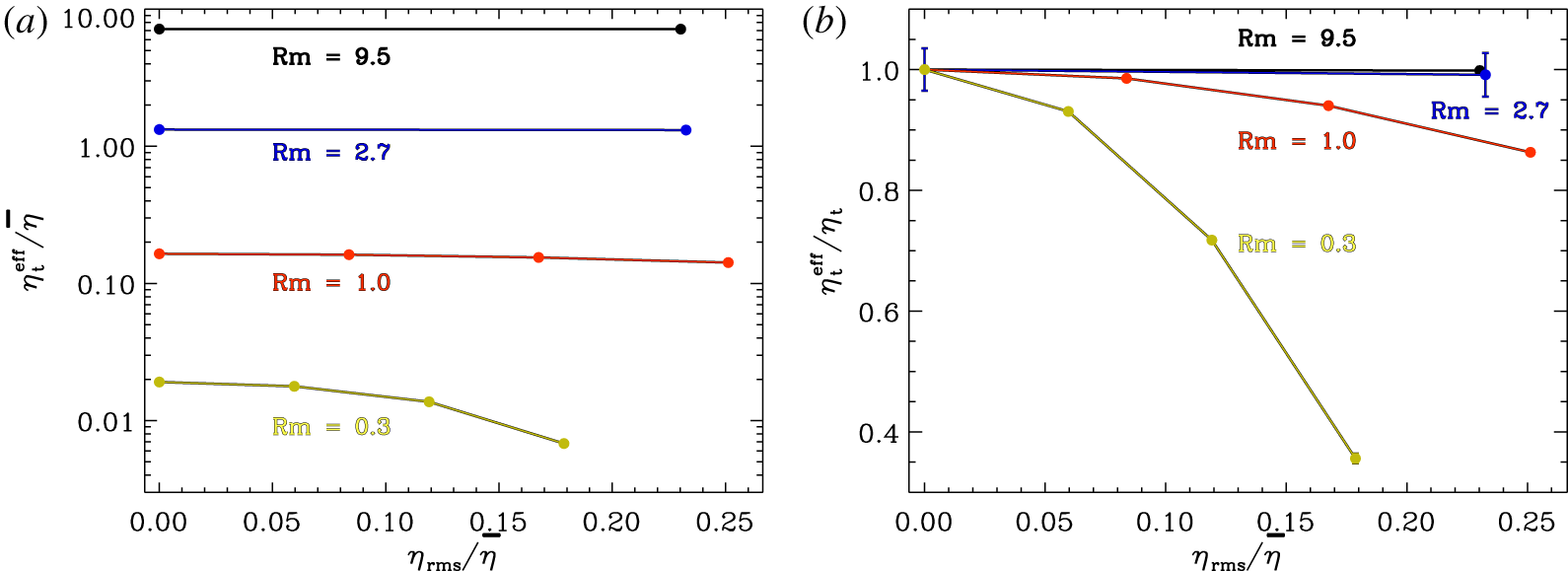
Figure 1. The specific diffusivity  $\unicode[STIX]{x1D702}_{\text{t}}^{\text{eff}}/\bar{\unicode[STIX]{x1D702}}$ (a) and the eddy diffusivity ratio
  $\unicode[STIX]{x1D702}_{\text{t}}^{\text{eff}}/\unicode[STIX]{x1D702}_{\text{t}}$ (b) as functions of the normalized diffusivity fluctuation
  $\unicode[STIX]{x1D702}_{\text{rms}}/\bar{\unicode[STIX]{x1D702}}$. In the high-conductivity limit (
 $Rm\gg 1$) the influence of the conductivity fluctuations disappears.
Going back to (2.22), we note that if the second expression is considered then its argument  $(\unicode[STIX]{x1D702}_{\text{rms}}/\bar{\unicode[STIX]{x1D702}})^{2}$ must be multiplied with
  $1/Rm$ for large
  $Rm$ and with
  $Rm^{0}$ for small
  $Rm$. It is thus clear that the diffusivity reduction by conductivity fluctuations disappears in the high-conductivity limit, which is confirmed by the numerical results, see figure 1(a). Figure 1(b) shows the numerical results for the ratio
  $\unicode[STIX]{x1D702}_{\text{t}}^{\text{eff}}/\unicode[STIX]{x1D702}_{\text{t}}$ of the terms in (2.22) which, of course, is unity for vanishing
  $\unicode[STIX]{x1D702}_{\text{rms}}$. It is also unity for large
  $Rm$ as the
  $\unicode[STIX]{x1D702}$-fluctuation-induced second term in (2.22) vanishes with
  $1/Rm$. Its role, however, becomes more important for small
  $Rm$. In this case, the first term loses its dominance and the total diffusivity
  $\unicode[STIX]{x1D702}_{\text{t}}^{\text{eff}}$ is reduced. If the numbers of figure 1(b) are multiplied with
  $\unicode[STIX]{x1D702}_{\text{t}}/\bar{\unicode[STIX]{x1D702}}$ then panel (a) results where the total magnetic diffusivity normalized with the microscopic value
  $\bar{\unicode[STIX]{x1D702}}$ is given. The influence of the conductivity fluctuations vanishes for large
  $Rm$ while the fluctuations provide smaller effective diffusivities
  $\unicode[STIX]{x1D702}_{\text{t}}^{\text{eff}}$ so that the cycle frequencies of oscillating dynamo models are reduced (Roberts Reference Roberts1972), also characteristic growth and decay times become longer.
3 Alpha effect
All turbulent flows which are known to possess an alpha effect are helical due to an inhomogeneity in the rotating turbulence field subject to the influence of a density and/or turbulence-intensity stratificationFootnote 2. The product  $\boldsymbol{g}\boldsymbol{\cdot }\unicode[STIX]{x1D734}$ forms the pseudo-scalar on which the pseudo-tensor
  $\unicode[STIX]{x1D6FC}$ in the relation (2.8) bases. However, the turbulence model considered in this paper is homogeneous and anisotropic. As the anisotropy is only implicit, it is not trivial whether the influence of global rotation will lead to an alpha effect or not.
3.1 Quasilinear approximation
We start with (2.12) and include the influence of rotation by the transformation  $\hat{u} _{p}=D_{pq}\hat{u} _{q}$ with the rotation operator
 $$\begin{eqnarray}D_{ij}=\unicode[STIX]{x1D6FF}_{ij}+\frac{(2\boldsymbol{k}\boldsymbol{\cdot }\unicode[STIX]{x1D734}/k)}{-\text{i}\unicode[STIX]{x1D714}+\unicode[STIX]{x1D708}k^{2}}\unicode[STIX]{x1D716}_{ijp}\frac{k_{p}}{k}\end{eqnarray}$$
 in the linear approximation (Kitchatinov, Pipin & Rüdiger Reference Kitchatinov, Pipin and Rüdiger1994). The second term gives the influence of the basic rotation in the Fourier representation. As it should be, it is even in the wavenumber and odd in the angular velocity. The Levi-Civita tensor ensures that the term is invariant with respect to the transformation of the coordinate system. It follows that  $\hat{{\mathcal{J}}}_{i}=\unicode[STIX]{x1D716}_{isp}k_{j}k_{s}D_{pq}\hat{U} _{q}B_{j}/(-\text{i}\unicode[STIX]{x1D714}+\bar{\unicode[STIX]{x1D702}}k^{2})+\cdots$, and finally
 $$\begin{eqnarray}\boldsymbol{{\mathcal{J}}}=-\unicode[STIX]{x1D6FE}\boldsymbol{g}\times \boldsymbol{B}+\unicode[STIX]{x1D6FC}(4(\boldsymbol{B}\boldsymbol{\cdot }\unicode[STIX]{x1D734})\boldsymbol{g}-(\boldsymbol{g}\boldsymbol{\cdot }\boldsymbol{B})\unicode[STIX]{x1D734}-(\boldsymbol{g}\boldsymbol{\cdot }\unicode[STIX]{x1D734})\boldsymbol{B}),\end{eqnarray}$$
 where  $\unicode[STIX]{x1D6FE}$ is given by (2.14) and for the coefficient
  $\unicode[STIX]{x1D6FC}$ (related but not identical to the tensor
  $\unicode[STIX]{x1D6FC}$ in (2.8)) one finds
 $$\begin{eqnarray}\unicode[STIX]{x1D6FC}=\frac{2}{15}\iint \frac{(\unicode[STIX]{x1D708}\bar{\unicode[STIX]{x1D702}}k^{4}-\unicode[STIX]{x1D714}^{2})k^{2}u_{1}}{(\unicode[STIX]{x1D714}^{2}+\bar{\unicode[STIX]{x1D702}}^{2}k^{4})(\unicode[STIX]{x1D714}^{2}+\unicode[STIX]{x1D708}^{2}k^{4})}\,\text{d}\boldsymbol{k}\,\text{d}\unicode[STIX]{x1D714}.\end{eqnarray}$$
 For  $\unicode[STIX]{x1D708}=\bar{\unicode[STIX]{x1D702}}$ and for frequency spectra which monotonically decrease for increasing
  $\unicode[STIX]{x1D714}$ the frequency integral in (3.3) has the same sign as
  $u_{1}$ while it vanishes a for a spectrum (‘white noise’) which does not depend on the frequency
  $\unicode[STIX]{x1D714}$. Correlations of a white-noise spectrum possess zero correlation times so that, indeed, the rotational influence should vanish. The
  $\unicode[STIX]{x1D6FC}$ effect after (3.2) is highly anisotropic, its last term is the rotation-induced standard
  $\unicode[STIX]{x1D6FC}$ expression.
Both quantities  $\unicode[STIX]{x1D6FC}$ and
  $\unicode[STIX]{x1D6FE}$ are linearly running with the ratio
  $\unicode[STIX]{x1D702}_{\text{rms}}/\bar{\unicode[STIX]{x1D702}}$. In the low-conductivity limit (
 $Rm<1$) they are
 $$\begin{eqnarray}\frac{\unicode[STIX]{x1D6FE}}{u_{\text{rms}}}\simeq \frac{\unicode[STIX]{x1D702}_{\text{rms}}}{\bar{\unicode[STIX]{x1D702}}},\quad \frac{\unicode[STIX]{x1D6FE}}{\unicode[STIX]{x1D6FC}\unicode[STIX]{x1D6FA}}\simeq \frac{1}{Rm~(\unicode[STIX]{x1D70F}_{\text{corr}}\unicode[STIX]{x1D6FA})}\end{eqnarray}$$
 while in the high-conductivity limit ( $Rm>1$)
 $$\begin{eqnarray}\frac{\unicode[STIX]{x1D6FE}}{u_{\text{rms}}}\simeq \frac{\unicode[STIX]{x1D702}_{\text{rms}}}{\bar{\unicode[STIX]{x1D702}}}\frac{1}{Rm},\quad \frac{\unicode[STIX]{x1D6FE}}{\unicode[STIX]{x1D6FC}\unicode[STIX]{x1D6FA}}\simeq \frac{1}{\unicode[STIX]{x1D70F}_{\text{corr}}\unicode[STIX]{x1D6FA}}.\end{eqnarray}$$
 Both relations for the  $\unicode[STIX]{x1D6FC}$ terms taken for all
  $Pm=\unicode[STIX]{x1D708}/\bar{\unicode[STIX]{x1D702}}\leqslant 1$. The
  $\unicode[STIX]{x1D6FC}$ effect always needs rotation; both of the given coefficients are small. The dimensionless ratio
  $\hat{\unicode[STIX]{x1D6FE}}=\unicode[STIX]{x1D6FE}/\unicode[STIX]{x1D6FC}\unicode[STIX]{x1D6FA}$ of the pumping term
  $\unicode[STIX]{x1D6FE}$ and the
  $\unicode[STIX]{x1D6FC}$ effect indicate the ratio of off-diagonal and diagonal elements in the alpha tensor. For
  $\hat{\unicode[STIX]{x1D6FE}}>1$, dynamo operation can highly be disturbed. For a standard disk dynamo Rüdiger, Elstner & Schultz (Reference Rüdiger, Elstner and Schultz1993) demonstrated with numerical simulations that large values of
  $|\hat{\unicode[STIX]{x1D6FE}}|$ suppress the dynamo action. In spherical dynamo models the
  $\unicode[STIX]{x1D738}$ term plays the role of an upward buoyancy (Moss, Tuominen & Brandenburg Reference Moss, Tuominen and Brandenburg1990) or even a strong downward turbulent pumping (Brandenburg, Moss & Tuominen Reference Brandenburg, Moss, Tuominen and Harvey1992). In order to be relevant for dynamo excitation, the
  $\unicode[STIX]{x1D6FC}$ effect should numerically exceed the value
  $\unicode[STIX]{x1D6FE}$ of the pumping term. As the pumping effect exists even for
  $\unicode[STIX]{x1D6FA}=0$, the ratio
  $\hat{\unicode[STIX]{x1D6FE}}$ should decrease for faster rotation. With extensive numerical simulations Gressel et al. (Reference Gressel, Ziegler, Elstner and Rüdiger2008) derived values of order unity for interstellar turbulence driven by collective supernova explosions. For rotating magnetoconvection Ossendrijver, Stix & Brandenburg (Reference Ossendrijver, Stix and Brandenburg2001), Ossendrijver et al. (Reference Ossendrijver, Stix, Brandenburg and Rüdiger2002) also found
  $\hat{\unicode[STIX]{x1D6FE}}\simeq 1$, where both
  $\unicode[STIX]{x1D6FC}$ and
  $\unicode[STIX]{x1D6FE}$ reached approximately 10 % of the root-mean-square value of the convective velocity. In their simulations of turbulent magnetoconvection Käpylä, Korpi & Brandenburg (Reference Käpylä, Korpi and Brandenburg2009) also reached typical values of order unity for
  $\hat{\unicode[STIX]{x1D6FE}}$.
3.2 Turbulent transport of electric current
We shall demonstrate why the existence of a diamagnetic pumping and an  $\unicode[STIX]{x1D6FC}$ effect for rotating but unstratified fluids with fluctuating diffusivity (in a fixed direction) is not too surprising. We start with the flow–current correlation
  $\langle \boldsymbol{u}^{\prime }\boldsymbol{\cdot }\text{curl}\,\boldsymbol{B}^{\prime }\rangle$ describing a turbulent transport of electric current fluctuations which after (2.12) for non-rotating turbulence certainly vanishes. This is not true for rotating turbulence as
  $\langle \boldsymbol{u}^{\prime }\boldsymbol{\cdot }\text{curl}\,\boldsymbol{B}^{\prime }\rangle \propto \bar{\boldsymbol{B}}\boldsymbol{\cdot }\unicode[STIX]{x1D734}$ is a possible construction for isotropic turbulence fields which only vanishes for
  $\bar{\boldsymbol{B}}\bot \unicode[STIX]{x1D734}$. Moreover, the tensor
  $\langle u_{i}^{\prime }\text{curl}_{j}\,\boldsymbol{B}^{\prime }\rangle$ for rotating isotropic turbulence may be written as
 $$\begin{eqnarray}\langle u_{i}^{\prime }\,\text{curl}_{j}\,\boldsymbol{B}^{\prime }\rangle =\unicode[STIX]{x1D705}_{1}\unicode[STIX]{x1D6FA}_{i}\bar{B}_{j}+\unicode[STIX]{x1D705}_{2}\unicode[STIX]{x1D6FA}_{j}\bar{B}_{i}+\unicode[STIX]{x1D705}_{3}(\unicode[STIX]{x1D734}\boldsymbol{\cdot }\bar{\boldsymbol{B}})\unicode[STIX]{x1D6FF}_{ij}.\end{eqnarray}$$
 In opposition to the tensors forming the helicity, the current helicity and the cross-helicity, the tensor (3.6) is not a pseudo-tensor and there is no reason that the dimensionless coefficients  $\unicode[STIX]{x1D705}_{i}$ identically vanish. The correlation
  $\langle u_{r}^{\prime }\,\text{curl}_{\unicode[STIX]{x1D719}}\,\boldsymbol{B}^{\prime }\rangle$ describes the up- or downward flow of azimuthal electric current fluctuations in a rotating magnetized turbulence. Imagine that
  $u_{r}^{\prime }$ is correlated (or anticorrelated) with fluctuations
  $\unicode[STIX]{x1D702}^{\prime }$ of the magnetic diffusivity, i.e.
  $\langle u_{r}^{\prime }\,\text{curl}_{\unicode[STIX]{x1D719}}\,\boldsymbol{B}^{\prime }\rangle \propto \langle \unicode[STIX]{x1D702}^{\prime }\,\text{curl}_{\unicode[STIX]{x1D719}}\,\boldsymbol{B}^{\prime }\rangle$ which is proportional to
  ${\mathcal{J}}_{\unicode[STIX]{x1D719}}$. If this quantity occurs for rotating turbulence under the influence of an azimuthal magnetic background
  $\bar{B}_{\unicode[STIX]{x1D719}}$ field then the existence of a new
  $\unicode[STIX]{x1D6FC}$ effect has been proven.
The calculation on the basis of (2.7) and (3.1) for rotating and magnetized but otherwise isotropic turbulence leads to the tensor expression
 $$\begin{eqnarray}\langle u_{i}^{\prime }\,\text{curl}_{j}\,\boldsymbol{B}^{\prime }\rangle =\unicode[STIX]{x1D705}(\unicode[STIX]{x1D6FA}_{i}\bar{B}_{j}+\unicode[STIX]{x1D6FA}_{j}\bar{B}_{i}-4(\unicode[STIX]{x1D734}\boldsymbol{\cdot }\bar{\boldsymbol{B}})\unicode[STIX]{x1D6FF}_{ij}),\end{eqnarray}$$
which is symmetric in its indices. One finds
 $$\begin{eqnarray}\unicode[STIX]{x1D705}=\frac{1}{30}\iint \frac{(\unicode[STIX]{x1D708}\bar{\unicode[STIX]{x1D702}}k^{4}-\unicode[STIX]{x1D714}^{2})k^{2}E}{(\unicode[STIX]{x1D714}^{2}+\bar{\unicode[STIX]{x1D702}}^{2}k^{4})(\unicode[STIX]{x1D714}^{2}+\unicode[STIX]{x1D708}^{2}k^{4})}\,\text{d}k\,\text{d}\unicode[STIX]{x1D714}.\end{eqnarray}$$
 The dimensionless  $\unicode[STIX]{x1D705}$ is almost identical to the integral (3.3); it is also positive for monotonically decreasing frequency spectra (at least for
  $\unicode[STIX]{x1D708}=\bar{\unicode[STIX]{x1D702}}$). For
  $\bar{\unicode[STIX]{x1D702}}\rightarrow 0$ one formally finds for the integrals
  $\unicode[STIX]{x1D705}\simeq St^{2}/15$ where the Strouhal number
  $St=u_{\text{rms}}\unicode[STIX]{x1D70F}_{\text{corr}}/\ell$, with
  $\ell$ being the correlation length. In the low-conductivity limit it runs with
  $Rm^{2}$.
On the other hand, without rotation the tensor (3.7) of the homogeneous turbulence can simply be written as  $\langle u_{i}^{\prime }\,\text{curl}_{j}\,\boldsymbol{B}^{\prime }\rangle =\unicode[STIX]{x1D705}^{\prime }\unicode[STIX]{x1D716}_{jik}\bar{B}_{k}$. As it should, the tensor is invariant against the simultaneous transformation
  $i\rightarrow j$ and
  $\bar{B}_{k}\rightarrow -\bar{B}_{k}$. Then
  $\langle (\boldsymbol{g}\boldsymbol{\cdot }\boldsymbol{u}^{\prime })\text{curl}\,\boldsymbol{B}^{\prime }\rangle =\unicode[STIX]{x1D705}^{\prime }\boldsymbol{g}\times \bar{\boldsymbol{B}}$ for all directions
  $\boldsymbol{g}$, hence
 $$\begin{eqnarray}\langle u_{r}^{\prime }\text{curl}_{\unicode[STIX]{x1D703}}\,\boldsymbol{B}^{\prime }\rangle =-\unicode[STIX]{x1D705}^{\prime }\bar{B}_{\unicode[STIX]{x1D719}}\end{eqnarray}$$
 for azimuthal background fields. After the heuristic replacement of  $u_{r}^{\prime }$ by
  $\unicode[STIX]{x1D702}^{\prime }$,
  $\unicode[STIX]{x1D705}^{\prime }$ in (3.9) stands for the new pumping term discussed above. The coefficient
 $$\begin{eqnarray}\unicode[STIX]{x1D705}^{\prime }=\frac{1}{15}\iint \frac{\bar{\unicode[STIX]{x1D702}}k^{4}E}{\unicode[STIX]{x1D714}^{2}+\bar{\unicode[STIX]{x1D702}}^{2}k^{4}}\,\text{d}k\,\text{d}\unicode[STIX]{x1D714},\end{eqnarray}$$
 which is of the dimension of the inverse of the correlation time, is positive–definite. In the formal limit  $\bar{\unicode[STIX]{x1D702}}\rightarrow 0$ the integral yields
  $\unicode[STIX]{x1D705}^{\prime }\simeq (2/15)St^{2}/\unicode[STIX]{x1D70F}_{\text{corr}}$ whereas in the low-conductivity limit it runs with
  $Rm$. We shall further demonstrate by numerical simulations that the correlations (3.7) and (3.9) indeed exist and that the coefficients
  $\unicode[STIX]{x1D705}$ and
  $\unicode[STIX]{x1D705}^{\prime }$ are positive.
3.3 Rotating magnetoconvection
A nonlinear numerical simulation with an existing code demonstrates the existence of the scalar quantities  $\unicode[STIX]{x1D705}^{\prime }$ and
  $\unicode[STIX]{x1D705}$ and, therefore, the existence of the pumping term (2.14) and the new
  $\unicode[STIX]{x1D6FC}$ effect. To this end the correlations
  $\langle u_{r}^{\prime }\text{curl}_{\unicode[STIX]{x1D703}}\,\boldsymbol{B}^{\prime }\rangle$ and
  $\langle u_{r}^{\prime }\text{curl}_{\unicode[STIX]{x1D719}}\,\boldsymbol{B}^{\prime }\rangle$ are calculated without and with rotation, yielding
  $\unicode[STIX]{x1D705}^{\prime }$ and
  $\unicode[STIX]{x1D705}$. As the latter correlation needs global rotation to exist,
  $\unicode[STIX]{x1D705}$ and, therefore, the
  $\unicode[STIX]{x1D6FC}$ effect, also need global rotation to exist.
A convectively unstable Cartesian box penetrated by an azimuthal magnetic field (fulfilling pseudo-vacuum boundary conditions at the top and bottom of the box) is considered with both density and temperature stratifications of (only) 10 %. A detailed description of the magnetoconvection code has been published earlier (Rüdiger & Küker Reference Rüdiger and Küker2016). The box is flat: two units in the vertical direction and four units in the two horizontal directions, there are  $128\times 256\times 256$ grid points. In code units the molecular diffusivity is
  $\unicode[STIX]{x1D702}\simeq 6\times 10^{-3}$ and the resulting turbulence intensity
  $u_{\text{rms}}\simeq 0.7$. The convection cells are characterized by
  $\unicode[STIX]{x1D70F}_{\text{corr}}\simeq 0.6$, hence
  $Rm\lesssim 50$. The values are not varied for the various simulation runs. After the definitions the magnetic field
  $B_{\unicode[STIX]{x1D719}}=1$ would take 40 % of the equipartition value
  $B_{\text{eq}}=\sqrt{\unicode[STIX]{x1D707}_{0}\unicode[STIX]{x1D70C}}u_{\text{rms}}$.
Figure 2(a) gives the results of a numerical simulation for a non-rotating box penetrated by an azimuthal magnetic field. We find  $\unicode[STIX]{x1D705}^{\prime }>0$ in accordance with the result (3.10) obtained within the quasi-linear approximation. If additionally
  $u_{r}^{\prime }$ and
  $\unicode[STIX]{x1D702}^{\prime }$ are (say) positively correlated then (3.10) provides positive values of
  $\unicode[STIX]{x1D6FE}$ in accordance to (2.14). Multiplication of the numerical result in figure 2(a) with the computed correlation time leads to
  $\unicode[STIX]{x1D70F}_{\text{corr}}\unicode[STIX]{x1D705}^{\prime }\simeq 0.5$, in good agreement with the analytical result (3.10).
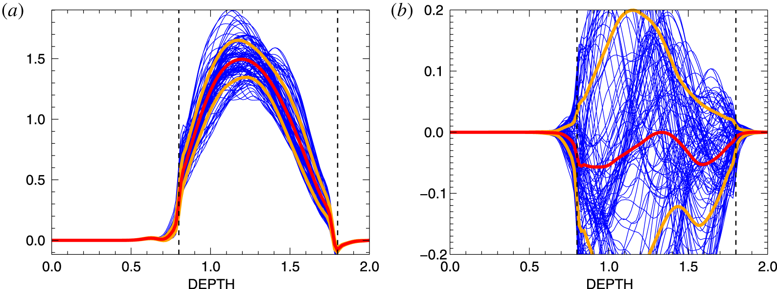
Figure 2. Snapshots of the turbulence-induced coefficients  $\unicode[STIX]{x1D705}^{\prime }$ after (3.9) (a) and the correlation (3.11) (b) from simulations of non-rotating convection with an azimuthal magnetic field. The convectively unstable region is located between the two vertical dashed lines, the red curves denote time averages and the yellow curves characterize the expectation value of the fluctuations. For non-rotating convection the correlation
  $\langle u_{r}^{\prime }\text{curl}_{\unicode[STIX]{x1D703}}\,\boldsymbol{B}^{\prime }\rangle$ exists but
  $\langle u_{r}^{\prime }\,\text{curl}_{\unicode[STIX]{x1D719}}\,\boldsymbol{B}^{\prime }\rangle$ vanishes.
  $B_{\unicode[STIX]{x1D719}}=1$,
  $\unicode[STIX]{x1D6FA}=0$,
  $Pm=0.1$.
From (3.7) it also follows that the tensor trace  $\langle \boldsymbol{u}^{\prime }\boldsymbol{\cdot }\text{curl}\,\boldsymbol{B}^{\prime }\rangle =-10\unicode[STIX]{x1D705}(\unicode[STIX]{x1D734}\boldsymbol{\cdot }\bar{\boldsymbol{B}})$ has a sign opposite to that of the correlation
  $\langle (\boldsymbol{g}\boldsymbol{\cdot }\boldsymbol{u}^{\prime })\text{curl}\,\boldsymbol{B}^{\prime }\rangle =\unicode[STIX]{x1D705}(\boldsymbol{g}\boldsymbol{\cdot }\unicode[STIX]{x1D734})\bar{\boldsymbol{B}}$, which we now consider for the hemisphere where
  $\boldsymbol{g}\boldsymbol{\cdot }\unicode[STIX]{x1D734}>0$. One finds that fluctuations of electric currents in the direction of the large-scale magnetic background field are correlated with the velocity component
  $\boldsymbol{g}\boldsymbol{\cdot }\boldsymbol{u}^{\prime }$, provided
  $\boldsymbol{g}$ is not perpendicular to the rotation axis. Hence,
 $$\begin{eqnarray}\langle u_{r}^{\prime }\,\text{curl}_{\unicode[STIX]{x1D719}}\,\boldsymbol{B}^{\prime }\rangle =\unicode[STIX]{x1D705}\cos \unicode[STIX]{x1D703}\unicode[STIX]{x1D6FA}\bar{B}_{\unicode[STIX]{x1D719}},\end{eqnarray}$$
 which means that in a rotating but otherwise isotropic turbulence with an azimuthal background field the radial flow fluctuations will always be correlated with azimuthal electric current fluctuations. The correlation (3.11) runs with  $\cos \unicode[STIX]{x1D703}$, it is thus antisymmetric with respect to the equator and it vanishes there. An upflow motion provides a positive (negative) azimuthal electric current fluctuation while a downflow motion provides a negative (positive) azimuthal electric current fluctuation so that the products of
  $u_{r}^{\prime }$ and
  $\text{curl}_{\unicode[STIX]{x1D719}}\,\boldsymbol{B}^{\prime }$ have the same sign in both cases. Replace now
  $u_{r}^{\prime }$ by
  $\unicode[STIX]{x1D702}^{\prime }$ and the existence of correlations such as
  $\langle \unicode[STIX]{x1D702}^{\prime }\text{curl}_{\unicode[STIX]{x1D719}}\,\boldsymbol{B}^{\prime }\rangle$ becomes obvious in rotating isotropic turbulence fields magnetized with an azimuthal background field. Just this finding is formulated by (2.4) and (3.2). Hence, the dimensionless coefficient
  $\unicode[STIX]{x1D705}$ in (3.11) is a proxy of an
  $\unicode[STIX]{x1D6FC}$ effect which appears when
  $u_{r}^{\prime }$ and
  $\unicode[STIX]{x1D702}^{\prime }$ are correlated or anticorrelated.
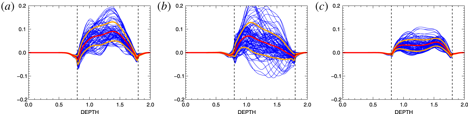
Figure 3. The values of  $\unicode[STIX]{x1D705}$ after (3.11) for rotating magnetoconvection with azimuthal magnetic field
  $B_{\unicode[STIX]{x1D719}}=\pm 1$ (a),
  $B_{\unicode[STIX]{x1D719}}=2$ (b) and
  $B_{\unicode[STIX]{x1D719}}=3$ (c).
  $\unicode[STIX]{x1D6FA}=3$,
  $Pm=0.1$,
  $\unicode[STIX]{x1D703}=45^{\circ }$.
We calculate  $\unicode[STIX]{x1D705}$ for different magnetic background fields for a fixed rotation rate. Figure 2(b) confirms that the correlation (3.11) vanishes for
  $\unicode[STIX]{x1D6FA}=0$. The three examples given in figure 3 have been computed with the rotation rate
  $\unicode[STIX]{x1D6FA}=3$ which corresponds to a Coriolis number
  $2\unicode[STIX]{x1D70F}_{\text{corr}}\unicode[STIX]{x1D6FA}=3.6$. The preferred direction
  $\boldsymbol{g}$ has been fixed to
  $\unicode[STIX]{x1D703}=45^{\circ }$ corresponding to mid-latitudes in a spherical geometry. These are natural choices as equator and poles as the two extremes are excluded. At the equator we do not expect finite correlations to exist while the simulations often meet complications at the poles. As expected, the resulting
  $\unicode[STIX]{x1D705}$ is positive and does not depend on the sign of the magnetic field. It is approximately
  ${\lesssim}0.1$ for weak magnetic fields. Due to magnetic suppression an increase of the field by a factor of three reduces the
  $\unicode[STIX]{x1D705}$ by the same factor. An estimation of the analytical result (3.8) yields
  $\unicode[STIX]{x1D705}\simeq (1/15)St^{2}$ for
  $\unicode[STIX]{x1D708}=\bar{\unicode[STIX]{x1D702}}$. Hence,
  $\unicode[STIX]{x1D705}\lesssim 0.1$ for a Strouhal number of unity derived from the analytical expressions is confirmed by numerical calculations. For the effective pumping
  $\hat{\unicode[STIX]{x1D6FE}}=\unicode[STIX]{x1D6FE}/\unicode[STIX]{x1D6FC}\unicode[STIX]{x1D6FA}$ the simulations provide the numerical value of
  $O(10)$ in (rough) accordance with the estimates (3.5).
For our argument only standard mean-field electrodynamics in turbulent media is needed. We note that the  $\unicode[STIX]{x1D6FC}$ term in (3.2) is turbulence originated but it does not need a prescribed helicity in stratified turbulent media; the helicity parameter
  $H$ from (2.18) does not occur in the calculations. In order to ensure the
  $\unicode[STIX]{x1D6FC}$ tensor is a pseudo-tensor the new
  $\unicode[STIX]{x1D6FC}$ effect only exists in rotating media which, however, are no longer required to be stratified in density and/or turbulent intensity.
The dynamo number  $C_{\unicode[STIX]{x1D6FC}}=|\unicode[STIX]{x1D6FC}|R/\unicode[STIX]{x1D702}_{\text{t}}$ for large
  $Rm$ is
 $$\begin{eqnarray}C_{\unicode[STIX]{x1D6FC}}\lesssim \frac{St}{Rm}\frac{\unicode[STIX]{x1D702}_{\text{rms}}}{\bar{\unicode[STIX]{x1D702}}}\frac{\unicode[STIX]{x1D6FA}R}{u_{\text{rms}}},\end{eqnarray}$$
 with  $R$ the characteristic size of the dynamo domain. That
  $C_{\unicode[STIX]{x1D6FC}}$ exceeds unity, which is necessary for dynamo excitation in
  $\unicode[STIX]{x1D6FC}^{2}$ models, cannot be excluded for sufficiently rapidly rotating large volumes. Applying the characteristic values of the geodynamo with
  $Rm\simeq 100$ and
  $u_{\text{rms}}\simeq 0.05~\text{cm}~\text{s}^{-1}$ would provide
  $\unicode[STIX]{x1D702}_{\text{rms}}/\bar{\unicode[STIX]{x1D702}}\gtrsim 10^{-4}$ as the excitation condition of an
  $\unicode[STIX]{x1D6FC}^{2}$-dynamo. We shall see below that in the outer core of the Earth such (large) values are not realistic. In the solar convection zone the equatorial velocity
  $\unicode[STIX]{x1D6FA}R$ slightly exceeds the maximal convection velocity but the very large
  $Rm$ will prevent sufficiently high values of
  $C_{\unicode[STIX]{x1D6FC}}$. The smallness of the presented
  $\unicode[STIX]{x1D6FC}$ effect does not prevent the operation of
  $\unicode[STIX]{x1D6FC}\unicode[STIX]{x1D6FA}$ dynamo models if sufficiently strong differential rotation exists. The standard solutions of these models, however, are oscillating with time scales of the order of the diffusion time.
Finally, it might be underlined that (3.11) describes a general turbulence-induced radial transport of azimuthal electric current fluctuations which vanishes for  $\unicode[STIX]{x1D6FA}=0$. It exists for all rotating homogeneous turbulence fields without another preferred direction beyond the rotation axis and magnetic field direction.
4 Results and discussion
We have shown analytically and with numerical simulations that the eddy diffusivity in a turbulent fluid is reduced if not only the flow speed but also the electric conductivity fluctuates. In this case the effective eddy diffusivity is smaller than that without diffusivity fluctuations. This is understandable as the large-scale electric current prefers the high-conductivity islands if they randomly exist in the fluid. For small magnetic Reynolds number  $Rm$ the large-scale diffusivity decreases with growing
  $\unicode[STIX]{x1D702}_{\text{rms}}/\bar{\unicode[STIX]{x1D702}}$ but this effect disappears for large
  $Rm$. Figure 1 demonstrates the reduction effect as a phenomenon of (say) a few 10 %.
If the fluid becomes anisotropic in the sense that one of the components of the flow vector is correlated (or anticorrelated) with the local values of the fluctuating electric conductivity then further phenomena appear. Convection may serve as an example where the downward and upward flows always have different temperatures and, therefore, different electric conductivities. If we define in positive radial direction the correlations as positive then a downward topological pumping of the magnetic field appears in the negative radial direction. In other words, if by the existence of correlations the diffusivity fluctuations are transported in one direction then the magnetic background field is transported in the opposite direction. This is despite the fact that the considered turbulence is homogeneous. Applying the diffusivity relation  $\unicode[STIX]{x1D702}\propto T^{-3/2}$ (Spitzer Reference Spitzer1962) to convection then the correlation
  $\langle \unicode[STIX]{x1D702}^{\prime }u_{r}^{\prime }\rangle$ (with
  $r$ as the radial direction in spheres) is negative. It formally describes a downward transport of diffusivity and hence the magnetic pumping should go upwards. The amplitude of the pumping velocity, however, is only a few per cent of the turbulent velocity which may be smaller by one order of magnitude than the diamagnetic effect of inhomogeneous turbulence.
The Spitzer relation yields  $\unicode[STIX]{x1D702}^{\prime }/\bar{\unicode[STIX]{x1D702}}\simeq -1.5T^{\prime }/T$, where a simple estimate provides
  $T_{\text{rms}}/T\simeq u_{\text{rms}}^{2}/g\ell$ with
  $g$ as the acceleration due to gravity. The numerical results
  $u_{\text{rms}}\simeq 0.7$ and
  $\ell \simeq 0.5$ provide
  $T_{\text{rms}}/T\simeq 5\times 10^{-4}$, in excellent agreement with the outcome of the numerical simulations (figure 4). The fluctuating diffusivity
  $\unicode[STIX]{x1D702}_{\text{rms}}/\bar{\unicode[STIX]{x1D702}}$ is of the same order, which after (3.12) is consistent with
  $C_{\unicode[STIX]{x1D6FC}}=O(1)$ if characteristics of the Earth’s core are applied. However, the very slow convection flows in the outer core of the Earth provide much smaller values of
  $\unicode[STIX]{x1D702}_{\text{rms}}/\bar{\unicode[STIX]{x1D702}}\simeq u_{\text{rms}}^{2}/g\ell \lesssim 10^{-12}$.
If the values of our local convection simulations are used to compute (3.12) then  $C_{\unicode[STIX]{x1D6FC}}\simeq 10^{-5}$, which is far from the possibility of exciting an
  $\unicode[STIX]{x1D6FC}^{2}$ dynamo.
Also, in the bulk of the solar convection zone the temperature fluctuations with  $T_{\text{rms}}/T\simeq 10^{-6}$ are small. Only the granulation pattern near the solar surface exhibits higher values of order 0.01 (Stix Reference Stix1989).
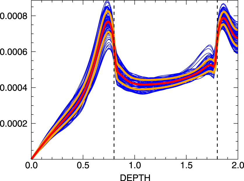
Figure 4. Similar to figure 3(a) but for the normalized temperature fluctuation  $T_{\text{rms}}/T$.
  $B_{\unicode[STIX]{x1D719}}=1$.
  $\unicode[STIX]{x1D6FA}=3$,
  $Pm=0.1$,
  $\unicode[STIX]{x1D703}=45^{\circ }$.
All previously known turbulence models which produce an  $\unicode[STIX]{x1D6FC}$ effect under the influence of rotation are inhomogeneous. The turbulence considered in the present paper is homogeneous but anisotropic if molecular diffusivity fluctuations are correlated (or anticorrelated) with the radial (better: upward and downward) velocity fluctuations. With the vector of the preferred direction (say
  $\boldsymbol{g}$) in the turbulence field one can form a pseudo-scalar
  $(\boldsymbol{g}\boldsymbol{\cdot }\unicode[STIX]{x1D734})$ which is needed for the existence of the pseudo-scalar
  $\unicode[STIX]{x1D6FC}$ in (2.8). It is thus challenging to probe our model for generation of an
  $\unicode[STIX]{x1D6FC}$ effect under the influence of rotation. Equations (3.2) and (3.3) represent the analytical results of a quasi-linear approximation. The coefficient
  $\unicode[STIX]{x1D6FC}$ has the same sign as the diffusivity–velocity correlation for
  $\unicode[STIX]{x1D6FF}$-like frequency spectra but it vanishes for white-noise (in time) spectra. The ratio
  $\hat{\unicode[STIX]{x1D6FE}}$ of the pumping term and the
  $\unicode[STIX]{x1D6FC}$ effect depends on the rotation rate. We estimate this ratio to be
  ${\lesssim}10$ for Coriolis number unity.
We have probed the properties of the diffusivity–current correlation vector  $\langle \unicode[STIX]{x1D702}^{\prime }\text{curl}\,\boldsymbol{B}^{\prime }\rangle$ by means of the proxy
  $\langle u_{r}^{\prime }\text{curl}\,\boldsymbol{B}^{\prime }\rangle$ where it is assumed that the flow component
  $u_{r}^{\prime }$ is correlated (or anticorrelated) with the diffusivity fluctuation
  $\unicode[STIX]{x1D702}^{\prime }$. To this end the turbulent flux of electric current (3.7) has been calculated under the influence of rotation and a uniform magnetic field in the azimuthal direction. With numerical simulations of rotating magnetoconvection driven by very weak density and temperature stratification, the analytical results have been verified. The interesting correlations are
  $\langle u_{r}^{\prime }\text{curl}_{\unicode[STIX]{x1D703}}\,\boldsymbol{B}^{\prime }\rangle$ for the pumping term
  $\unicode[STIX]{x1D6FE}$ and
  $\langle u_{r}^{\prime }\text{curl}_{\unicode[STIX]{x1D719}}\,\boldsymbol{B}^{\prime }\rangle$ for the
  $\unicode[STIX]{x1D6FC}$ term. We note that the considered turbulence field is non-helical. In opposition to the tensors of helicity
  $\langle u_{i}^{\prime }\text{curl}_{j}\,\boldsymbol{u}^{\prime }\rangle$ and current helicity
  $\langle B_{i}^{\prime }\text{curl}_{j}\,\boldsymbol{B}^{\prime }\rangle$, the current-flux tensor
  $\langle u_{i}^{\prime }\text{curl}_{j}\,\boldsymbol{B}^{\prime }\rangle$ is not a pseudo-tensor. Both correlations show finite values with the expected signs and with the correct symmetry properties.
Editor Steve Tobias thanks the referees for their advice in evaluating this article.


 Open access