Injection-Induced Seismic Risk Management Using Machine Learning Methodology – A Perspective Study
 Miao He
 Qi Li
Qi Li Xiaying Li1,2
- 1State Key Laboratory of Geomechanics and Geotechnical Engineering, Institute of Rock and Soil Mechanics, Chinese Academy of Sciences, Wuhan, China
- 2School of Engineering Science, University of Chinese Academy of Sciences, Beijing, China
Effective identification of induced seismicity and real-time management of seismic risks are hot topics due to increasing induced seismicity in areas related to energy exploitation. Existing decision-making tool for managing seismic risks, known as the traffic light system, is not robust enough. To meet the increasing needs for safe mining of energy at production sites, finding an advanced and efficient method to improve the traffic light system is essential. In recent years, machine learning, an advanced inductive and analytical method, has been widely used in seismology. In this context, research gaps associated with the identification and management of induced seismicity, as well as the current achievements of machine learning in addressing induced seismicity problems, are reviewed. A basic framework of using machine learning method to optimize the traffic light system in the industrial production process is first proposed. Then, its feasibility and rationality are demonstrated by similar cases. This framework may provide a reference for the development of a risk-based adaptive traffic light management system.
Highlights
– The progress and gaps in injection-induced seismicity are reviewed.
– The concepts and current challenges of traffic light systems are reviewed.
– The main methods of machine learning and their applications in induced seismicity are summarized.
– The basic framework for improving the traffic light system using machine learning method is proposed.
– The feasibility and rationality of the framework are demonstrated by similar cases.
Introduction
Earthquakes can cause the sudden release of elastic energy in the Earth. Generally, natural earthquakes are caused by crustal movements, and the majority of strong seismic events in the world are natural earthquakes and have tectonic origin. Unlike natural earthquakes, most induced seismic events are usually related to anthropogenic production activities. The mechanisms that account for induced seismicity include changes in the state of stress, pore pressure, volume, and applied forces or loads (McGarr et al., 2002). The earliest induced earthquake records can be traced back to the 1920s (Pratt and Johnson, 1926), and the most classic case of wastewater reinjection-induced seismicity occurred in Denver, Colorado, in the 1960s (Evans, 1966; Healy et al., 1968; Hsieh and Bredehoeft, 1981).
The potential of energy technologies to induce earthquakes is known (National Research Council, 2013), mainly including wastewater disposal (e.g., Pratt and Johnson, 1926; Davis and Frohlich, 1993; Currie et al., 2018), extraction and injection of natural gas (e.g., Grasso and Wittlinger, 1990; Herber and de Jager, 2014; Zbinden et al., 2017), geothermal energy exploitation (e.g., Majer and Peterson, 2007; Martínez-Garzón et al., 2016; Boyd et al., 2018), hydraulic fracturing (e.g., Rutqvist et al., 2015; Bao and Eaton, 2016; Ghofrani and Atkinson, 2016) and Carbon dioxide (CO2) geological sequestration (Goertz-Allmann et al., 2014, 2017a,b). Frequently felt earthquakes (3 ≤ M < 4.5) can create negative public sentiments and even hinder the smooth progress of industrial production. For instance, in the Basel Geothermal Field, Switzerland, enhanced geothermal system (EGS) exploitation projects induced a series of locally felt earthquake events. The damage claims in Basel amounted to more than $9 million, and these projects were temporarily suspended due to strong protests from the general public (Giardini, 2009). A similar case occurred in the Groningen gas field, the Netherlands. In the 28 years since the gas was extracted in 1991, there have been approximately 320 earthquakes with M > 1.5, including 3 M≈3.5 earthquakes. These growing seismic events have caused widespread building damage, social concern and political upheaval (Sintubin, 2018; Vlek, 2018, 2019a,b). Moderate magnitude earthquakes (4.5 ≤ M < 6) may threaten public safety and cause heavy economic losses. For instance, in the Changning shale gas block, Sichuan Basin, China, a moderate intensity earthquake (ML 5.7) occurred on 16 December 2018. In this event, 17 persons were injured, more than 390 houses were damaged, and 9 houses collapsed. The direct economic loss reached approximately 50 million CNY (Lei et al., 2019). Another famous induced earthquake is the MW 5.5 Pohang earthquake. The earthquake occurred on 15 November 2017, in Heunghae, Pohang in the North Gyeongsang Province in South Korea (Kim et al., 2018). The earthquake injured 82 people, killed one and left about 1,500 homeless, moreover, it caused serious damage to infrastructure and more than 75 million US dollars (Ellsworth et al., 2019). More cases of human-induced seismicity can be found in some reports and papers (e.g., Gibson and Sandiford, 2013; Folger and Tiemann, 2017; Foulger et al., 2018). Therefore, managing the risks of induced seismicity is of great significance for the smooth progress of industrial production and the development of energy technology.
In recent years, due to the fossil energy crisis, more resources from deeper in the Earth are needed, and in turn, the induced seismicity becomes more prominent. Although the traffic light system (TLS) has been used to manage the risk of induced seismicity, there remain two unresolved problems at present: (1) the differences between natural and induced earthquakes cannot be completely distinguished; (2) the evolving risk of deep fluid injection-induced seismicity is still difficult to manage effectively and timely, especially in the post-injection phase after shut-in. To solve these two problems, many different types of data related to injection-induced seismicity are needed, including geological data, seismicity and operational parameters (Yang et al., 2017). Unfortunately, the characteristics of the induced seismicity and their relationships with the production parameters are usually hidden in these large and disorderly data, and we cannot extract effective information from the large amount of data merely by analytical or conventional methods.
The rapid development of computer science provides technical support for big data processing, especially machine learning techniques. Machine learning (ML) was proposed in the computational model theory of neural networks in the 1940s (McCulloch and Pitts, 1943). It is a computer algorithm that can automatically improve itself through experience (Mitchell, 1997), and also a transformation chain from data to decision. ML can use mathematical and statistical methods to determine the intrinsic regulation from various data. To date, it has evolved towards more advanced learning types that are closer to the human brain, such as deep learning (Hinton and Salakhutdinov, 2006), transfer learning (Pan and Yang, 2010) and deep reinforcement learning (Mnih et al., 2015). At the same time, ML has been widely used in many fields, especially in seismology, such as for the identification and prediction of earthquake events (e.g., Asim et al., 2016; DeVries et al., 2018; Lubbers et al., 2018; Rajguru et al., 2018; Corbi et al., 2019) and the classification of seismic remote sensing images (e.g., Afonso et al., 2016; Bialas et al., 2016; Frank et al., 2017), etc. However, the achievements in solving induced seismicity by using ML-based methods are rarely reported, especially in improving traffic light systems.
In this context, we attempt to propose a basic framework for improving current traffic light system that is, using machine learning method to build a proxy model. This model could well reflect the complex relationship between seismicity magnitude and operational parameters. The paper is organized as follows. The first section briefly reviews the research progress of induced earthquakes related to fluid injection, including the explanation of the mechanism, the discrimination of induced seismicity and the concept of the traffic light system. Then, the main methods of machine learning and their research achievements in induced seismicity are summarized and reviewed systematically. Finally, the basic framework of using machine learning method to optimize the traffic light system is elaborated.
Review of Fluid-Induced Seismicity
Fault reactivation induced by fluid injection in industrial activity is one of the main causes of seismicity (Ellsworth, 2013), and Figure 1 displays this process. Identified factors affecting fault reactivation mainly include the rate and volume of fluid injection (Nicol et al., 2011), in-situ stress conditions (Rutqvist et al., 2010), type and occurrence of the fault (Macdonald et al., 2012), and physical and mechanical properties of host rocks (Figueiredo et al., 2015). Notably, the most relevant role is played by fault orientation versus dominant stress orientation. In this section, the research progress and gaps in induced seismicity related to industrial activities are reviewed briefly.
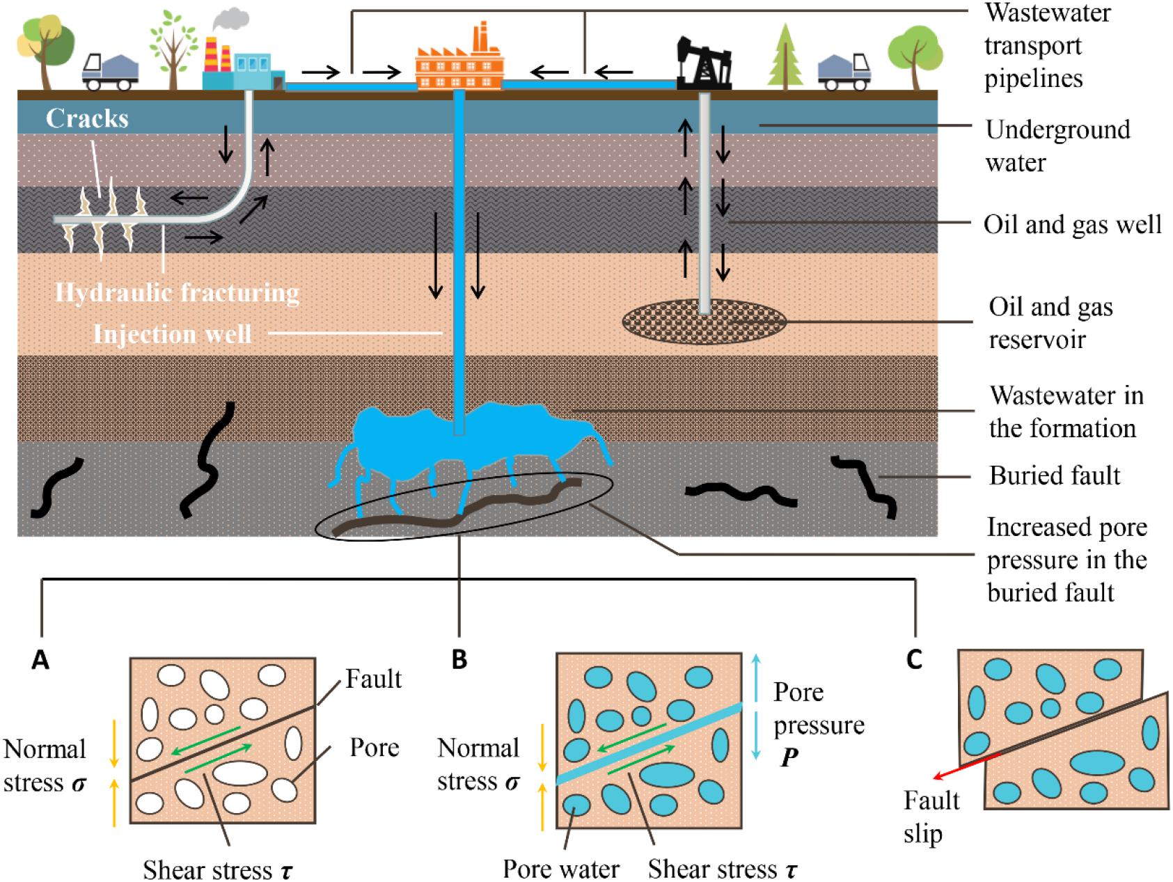
Figure 1. The whole process of fault slip induced by fluid injection in industrial production. (A) Before fluid injection, the fault is closed under the pressure of normal stress on both sides. (B) With the continuous injection of fluid during the production process, the pores and cracks in the fault are gradually filled with fluid. (C) When pore pressure increases to a certain value, the fault slips because the effective normal stress on both sides is less than the shear stress; then, an earthquake is induced.
Mechanisms of Induced Seismicity
The Coulomb failure criterion based on Mohr-Coulomb theory is commonly used to explain the mechanism of induced seismicity (Healy et al., 1968) and can be defined as:
where ΔCFS is Coulomb stress, Δτ is the shear stress change (MPa), μ is the friction coefficient on the fault, and Δσ′ is the effective normal stress change (MPa), which can be calculated according to the effective stress principle (Alcoverro, 2003):
where σ is the normal stress (MPa) and P is the pore pressure (MPa).
In Eq. (1), when ΔCFS > 0, the fault loses stability and fails; otherwise, it remains stable.
Based on different ways of fluid injection or extraction in industrial production, Doglioni (2018) further summarized four possible mechanisms, that is, fluid removal from a stratigraphic reservoir that can cause normal faults-related earthquakes (also called graviquakes), reinjection quakes, hydrofracturing quakes and load quakes, as shown in Figure 2. For a more detailed explanation of the mechanism of fluid-induced seismicity, please refer to Shapiro (2015).
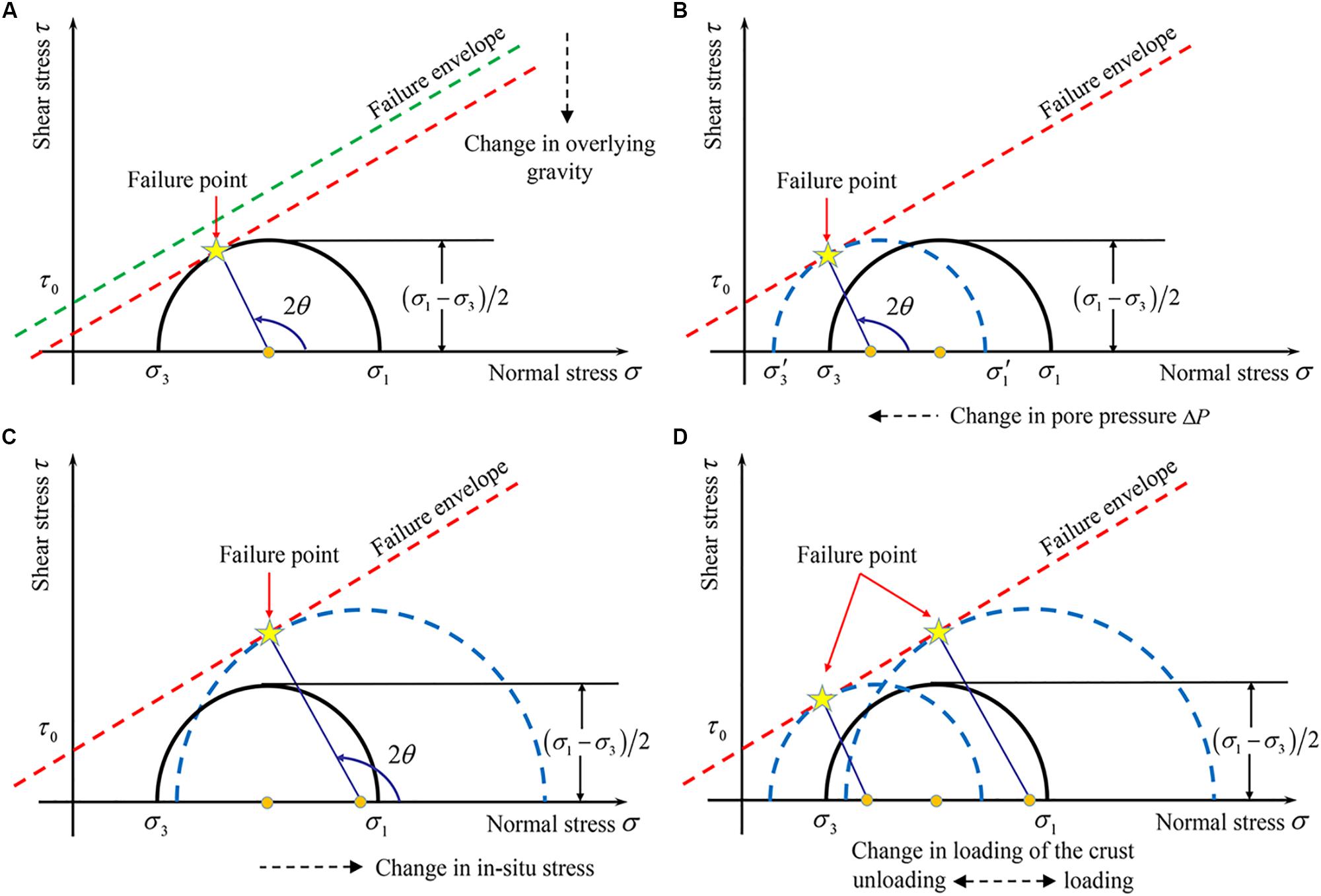
Figure 2. Fault failure is induced by four possible mechanisms: (A) graviquakes, (B) reinjection quakes, (C) hydrofracturing quakes, (D) load quakes. The black solid Mohr circles represent the in-situ stress state of the fault before industrial production, while the blue dashed circles show the stress state after different changes. The red dotted lines mark the failure envelope in the safe state, and the red corresponds to the critical state. The fault is considered to fail when the Mohr circle is tangent to the envelope (as shown by the yellow star). [Modified from Doglioni (2018)] (This work is licensed under the CC BY-NC-ND license. http://creativecommons.org/licenses/by-nc-nd/4.0/).
It is worth noting, however, that the Coulomb failure criterion can only be used to simply evaluate whether a fault is reactivated, and cannot truly reflect the entire physical process of fault failure induced by industrial activities.
Discrimination of Natural and Induced Seismicity
The first step for reducing seismic hazard is to effectively identify induced seismicity among a large number of earthquake events. Davis and Frohlich (1993) first proposed analytical approaches to discriminate between induced and natural earthquakes in industrial activity based on a set of YES or NO criteria. The analytical approaches for differentiation mainly include physics-based probabilistic models, statistics-based seismicity models and source parameter approaches (Dahm et al., 2012). Table 1 lists the basic information about these three discrimination methods, including theoretical bases, advantages, disadvantages, and application scopes.
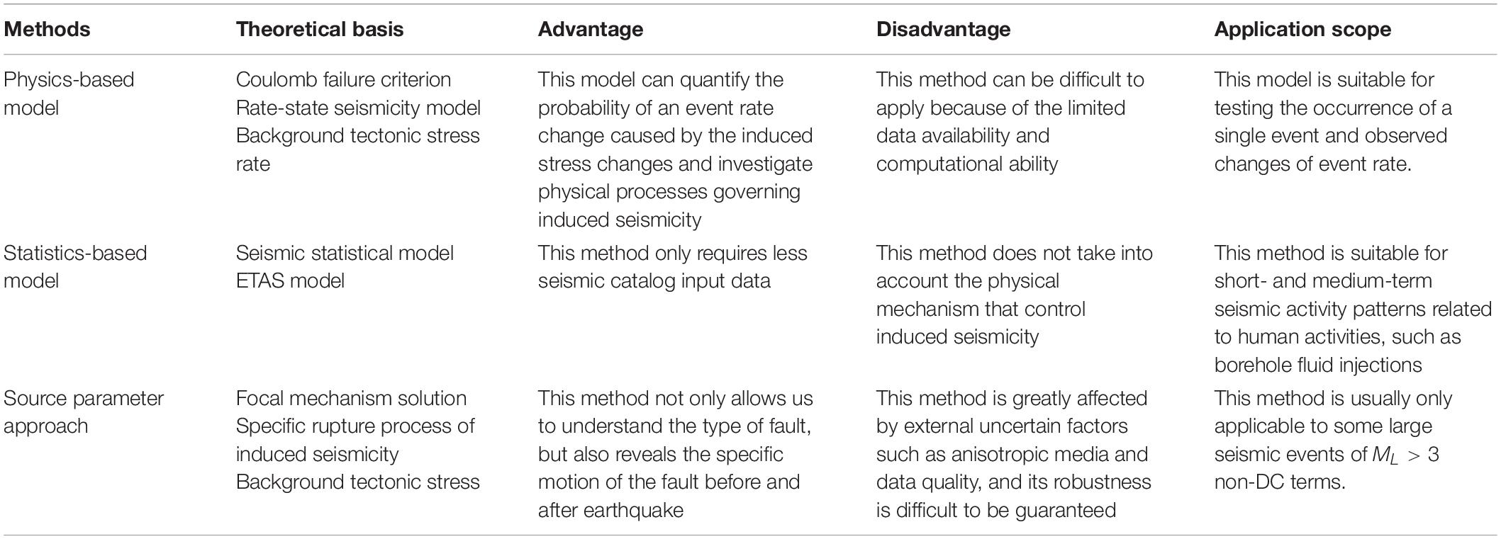
Table 1. Basic information of three different discrimination methods.
Physics-Based Probabilistic Model
The physics-based model is used to understand the complicated relationship between fluid migration and seismic activity and reveal the physical processes of induced seismicity by using laboratory and in-situ measurements and numerical simulations (e.g., Guglielmi et al., 2015; Zbinden et al., 2017). In recent years, physics-based probabilistic models have been developed, taking into account physical and statistical-stochastic factors (Dahm et al., 2015).
This model can be used to quantify the probability of event rate change induced by stress changes. However, it is not suitable in case of insufficiently detailed data, such as production/exploitation data and rock parameters (e.g., Passarelli et al., 2012; Rinaldi and Nespoli, 2017).
Statistics-Based Seismicity Model
The statistics-based seismicity model directly uses the change in statistical parameters in an earthquake catalog to determine whether the rate of stress change caused by production exceeds the change in natural stress. It is worth mentioning that the changes in these parameters are likely related to human activities. The epidemic-type aftershock sequence (ETAS) model (Hainzl and Ogata, 2005) is often used to identify artificial factors in seismicity event statistics.
The ETAS model is a combination of a constant background activity rate and the behavior of aftershock sequences according to the Omori-Utsu law (Tokuji et al., 1995). The total occurrence rate can be calculated by the sum of Omori’s law for aftershocks ν(t) and the background activity rate λ(t) (Lei et al., 2017):
where K0 is a constant, α is a constant related to the magnitude dependence, Mi is the magnitude of the i-th earthquake, Mc is the estimated cut-off magnitude of completeness, and are constants for Omori’s law.
When the background rate λ(t)≫50% and the Omori’s law aftershocks ν(t) are rare, the earthquake can be considered artificially induced (Lei et al., 2008, 2013, 2017, 2019). In recent years, improved statistical models have been proposed to forecast and discriminate induced seismicity in the space-time-magnitude domain (Gaucher et al., 2015; Zaliapin and Ben-Zion, 2016; Grigoli et al., 2017).
Statistics-based methods do not need to consider complex physical constraints, so their advantage is that few input data or detailed models are required.
Source Parameter Approach
The source parameter approach attempts to discriminate between induced and natural earthquakes by searching specific rupture processes. It is generally believed that the hypocentral locations of induced earthquakes are different in the range of human activities. The source mechanism solution obtained by moment tensor (MT) inversion helps in understanding the orientation and type of fault and obtaining the subsurface stress field disturbance caused by fluid injection (Grigoli et al., 2017).
The moment tensor inversion is an important physical quantity describing different types of earthquakes. It consists of double-couple (DC) and non-DC components, where the non-DC includes isotropic (ISO) components and compensated linear vector dipole (CLVD) components (Gilbert, 1971):
where MT is the moment tensor, which can be inversed by, Gf is Green’s function, and is the ground motion. When a high proportion of ISO and non-DC components occurs, an earthquake is likely to be induced because natural earthquakes are often characterized by a nearly pure DC source mechanism. This contrast provides an effective means to discriminate induced from natural seismicity (Cesca et al., 2012).
The moment tensor inversion is usually combined with other methods, such as waveform template matching (Skoumal et al., 2015), source spectra, and stress drop estimation (Clerc et al., 2016; Zhang et al., 2016). However, the source parameter approach requires high-quality data. If the structural model is not sufficiently accurate, a certain error appears in the analog waveform, and the results of waveform inversion may have significant deviations (Jechumtálová and Bulant, 2014).
It is worth noting that these three methods are often used in combination with detailed seismicity source parameters (Dahm et al., 2015). Some research cases and achievements in typical regions are given in Table 2.
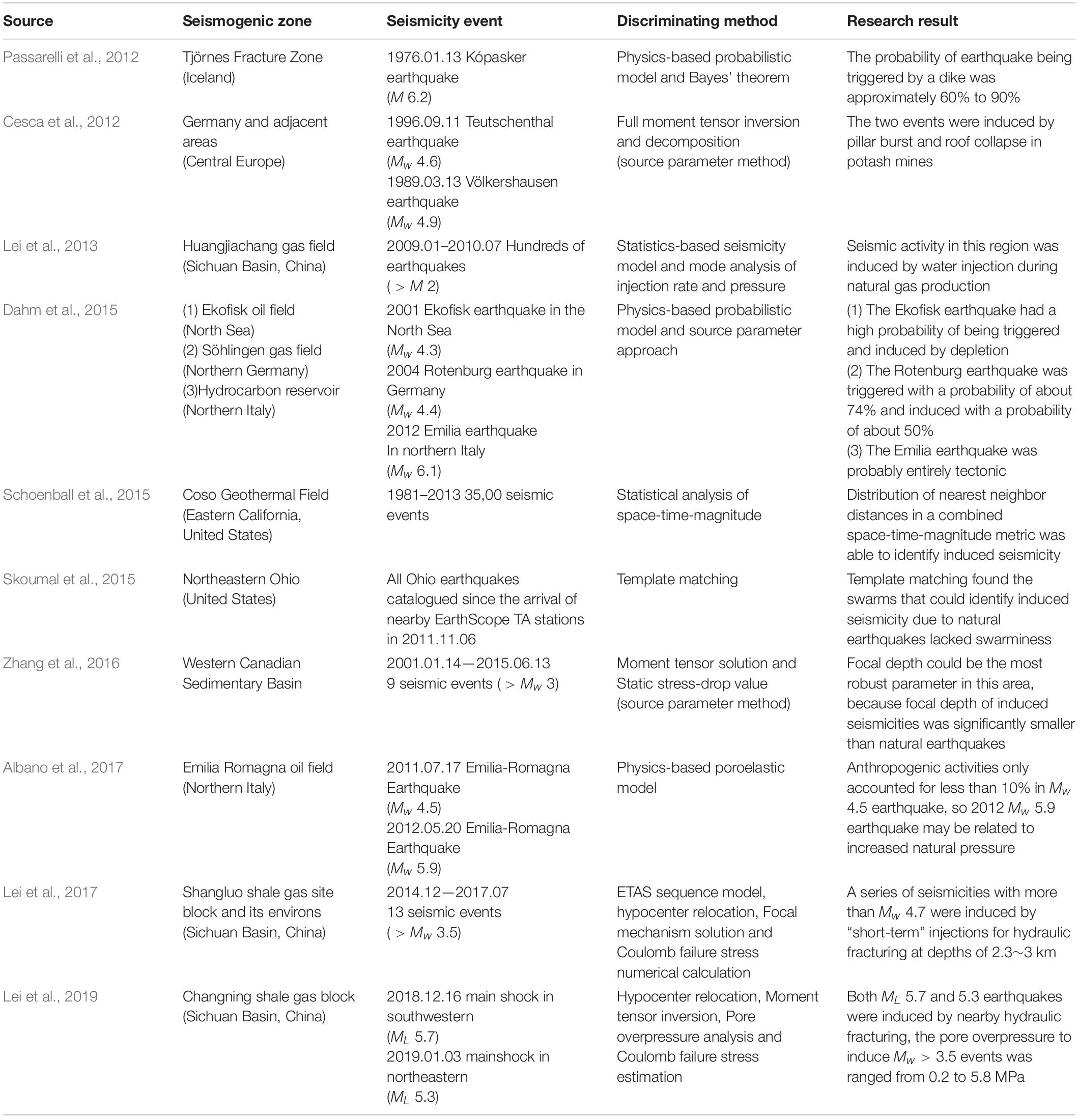
Table 2. Discrimination of natural and induced seismicity in some typical regions.
Relationship Between Operational Parameters and Seismicity Magnitude
The operational parameters of fluid injection, such as wellhead pressure, total injection volume, injection rate and injection location, are the important factors affecting fault reactivation. Understanding the relation between reservoir engineering operations and corresponding seismic response is important towards the optimization of production and mitigating seismic hazard (Hofmann et al., 2018).
Some scholars have built analytical models based on statistical methods. For instance, Nicol et al. (2011) conducted statistical analysis of water injection data and seismic data from the 30 best reported seismicity sites. They found that the magnitude was positively correlated with the fluid injection, which could be expressed as M = 0.3353lnΔV + 1.8061, where M is the earthquake magnitude and ΔV is the water injection volume. McGarr (2014) studied some earthquakes induced by unconventional oil and gas production in the central and eastern United States and found that the maximum magnitude seemed to be proportional to the total volume of the injected fluid but with an upper limit. Under some assumptions, which can be found in section 3 of McGarr (2014), the upper limit magnitude for a given fluid injection activity could be estimated as M0(max) = GΔV, where G is the shear modulus. Galis et al. (2017) analyzed a scaling relation between the largest magnitude of self-arrested earthquakes and the injected volume ΔV with an analytical model .
Numerical simulations are also used to predict the maximum seismic magnitude. Lei et al. (2017) studied the physical mechanisms of several moderate earthquake sequences in the Shangluo shale gas block and its environs (Sichuan Basin, China). They used the “TOUGH-FLAC” simulator to conduct coupled thermal-hydrological-mechanical (THM) analysis on the ΔCFS evolution patterns caused by hydraulic fracturing injection in this area. Based on it, a numerical model containing four layers of different mechanical and hydraulic properties was established, and the critical pressure at the injection wellhead that could cause fault failure was determined. Focusing on the different shale gas basins in North America, Amini and Eberhardt (2019) studied the effect of tectonic stress regime on the magnitude and its distribution of induced seismicity associated with hydraulic fracturing. They used the 3D distinct-element method to simulate the fault slip under different stress regimes, and found that both the shear displacement magnitudes and the stress drop for the thrust and reverse fault case were much larger than those for the normal and strike-slip fault case.
Notably, the prediction accuracy of these analytical models is highly dependent on the input parameters (Eaton and Igonin, 2018), and the relationship between operational parameters and seismicity magnitude may not always be simple or straight. In addition, numerical simulations might have problems with calibration when proper parameters are difficult to select.
Traffic Light System for Safe Production
The traffic light system (TLS) is a powerful decision-making tool to manage industrial activities (Bommer et al., 2006). This system has been widely used to manage a risk associated with operation-related earthquakes, often using two or more thresholds to mitigate unexpected seismic hazards (Baisch et al., 2019; Wei et al., 2020). In this section, the application and limitations of TLS in induced seismicity are reviewed.
Working Mechanisms and Application Cases
A TLS consists of decision variables (e.g., peak ground acceleration, peak ground velocity, earthquake magnitude and other parameters) and thresholds (Mignan et al., 2017). When the earthquake magnitude or ground shaking exceed the threshold, the alert levels will be automatically activated and relevant actions must be taken (e.g., stopping operations, reducing injection rate or volume) (Braun et al., 2020).
The TLS is usually divided into three alert levels to provide feedback to manage operational measures or actions. Figure 3 shows a workflow of the traffic light system. When the traffic light is green, conditions are normal, and production can continue as planned. When the light becomes orange, it means caution, and the operational parameters should be adjusted. However, if the light turns red, the production must be suspended.
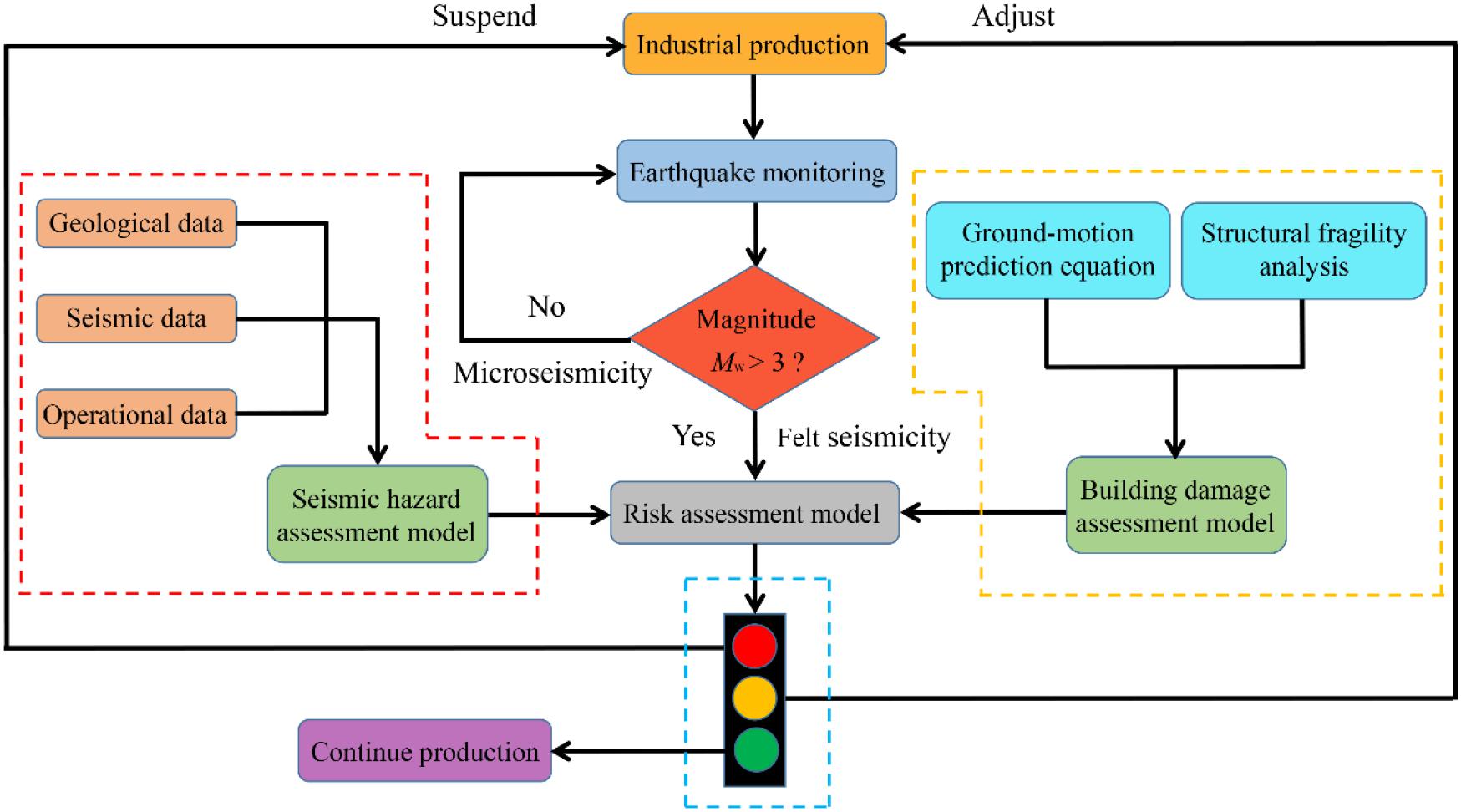
Figure 3. A complete workflow of the traffic light system. The traffic light system needs to make decisions based on the results of the risk assessment model, which consists of a seismic assessment model and a building damage assessment model. The judgment basis for the former model is magnitude, while that for the latter model is ground motion.
At present, the model of predicting piecewise induced seismic activity rateλ(t,M≥M0;θ)and the exceedance probability of risk assessment in TLS are as follows (Mignan et al., 2017):
where V(t) is the cumulative injected fluid volume (m3), is the injection flow rate (m3/day), θ(afb,bs,τr) is a set of model parameters describing the underground characteristics, afb is the activation feedback in m–3, bs is the earthquake size ratio, τr is the mean relaxation time in days, M0 is the minimum cut-off magnitude, tshut–in is the shut-in time (day), and Msaf is the given safety magnitude (i.e., threshold magnitude). Notably, Y represents the probability that the magnitude exceeds the threshold. Whenever the magnitude of an induced seismic event exceeds the threshold, Y = 1.
For different industrial activities, criteria for setting-up the TLS may be very different. Baisch et al. (2019) summarized some examples of existing TLS that correspond to different industrial activities taking place in Europe, North America and Australia, as shown in Figure 4. Notably, the wastewater disposal in the Cavone oil field is mainly used to enhance oil (or gas) production and to balance the loss of volume due to the primary production. It is within the production reservoir and is considered quite safe as regards induced seismicity (Styles et al., 2014).

Figure 4. Application cases of traffic light system (TLS) corresponding to different industrial activities in Europe, North America and Australia.
Meanwhile, Baisch et al. (2019) investigated the different effects of TLS on seismic activity caused by fluid injection and gas production based on observation data from 12 fluid-injection operations in geothermal reservoirs and gas production in 26 gas fields. Their research showed that, for an earthquake of a given strength, the effect of TLS on short-term fluid injection induced seismicity was significantly better than that of gas production-induced seismicity.
Current Limitations
Remarkably, in TLS, the decision variables such as magnitude, PGV, and possibly other parameters are linked each other, and which decision variable to choose depends on how they contribute to the risk evaluation. When the appropriate reference variables for the decision are selected, their corresponding thresholds need to be further determined. Unfortunately, there are some challenges in determining the threshold effectively and timely.
Take the threshold magnitude as an example. Threshold magnitude is the transitional magnitude between different alert levels. The relationship between threshold magnitudes and operational parameters plays a vital role in TLS. However, the current definition of threshold magnitude Msaf in Eq. (6) is mainly chosen on the basis of expert judgment and regulation (Grigoli et al., 2017; Mignan et al., 2017), which lacks objectivity and cannot reflect the full range of possible scenarios. Magnitude thresholds enforced by different jurisdictions may vary significantly. It would further result in TLS not being flexible enough to adapt to evolving risks. Therefore, at present, one of the main limitations of classical TLS is that the threshold magnitudes for different stages are difficult to reappraisal accurately and timely, especially in the post-injection phase.
An important lesson about the limitation of classical TLS has recently come from the Pohang earthquake. Notably, Woo et al. (2019) used a variety of methods including the construction of a velocity model, to conduct earthquake detection, the determination of hypocenters, magnitudes, focal mechanisms and stress inversion, and a clustering analysis, to conduct a seismic analysis on the earthquakes occurring around the EGS site in the past 10 years. It is worth noting that all those investigations were important in order to improve the seismological interpretation, which was needed for an effective application of TLS. As part of the EGS project, a clear causal relationship between the origin of the MW 5.5 Pohang earthquake and the injected fluid was discovered. That is, the earthquake initiated on the fault zone that was reactivated by fluid injection, representing a self-sustained rupture process that released a large amount of energy via tectonic loading rather than being a directly induced earthquake via fluid injection.
In the Pohang EGS project, the monitoring focus of classical TLS is the threshold magnitude. However, Ellsworth et al. (2019) and Lee et al. (2019) found that EGS stimulation could trigger large earthquakes that rupture beyond the stimulated volume, and the assumption that the maximum seismic magnitude was governed by the injection volume might no longer be true. It indicated that in addition to injection volume, more operational parameters should be considered in reappraising the threshold magnitude. Moreover, sufficient attention must be paid to post-injection seismicity after shut-in.
On the issue of post-injection earthquakes, Baisch et al. (2019) pointed out that the performance of TLS depends heavily on the prediction model that accounts for post-injection seismicity, so the post-injection phase must be considered in the design of TLS thresholds. The predicting model in Eq. (5) has the advantages of simplicity and stability, and can also consider the underground feedback in the post-injection phase. However, it assumes that the relationship between injection rate and overpressure is linear, and the fluid diffusion process at the post-injection phase is only represented by an exponential decay, which is different from the actual physical process (Mignan et al., 2017). In addition, the magnitude used in post-injection model does not change with time and cannot meet the real-time design of TLS thresholds in the post-injection phase.
Based on the 2017 Pohang earthquake experience, it is urgent to develop risk-based TLS based on the relationship between EGS and associated stimulus activities to adapt to evolving hazards. To this end, physical and statistical models of induced and triggered seismicity were also needed to further develop, as well as some advanced analyses. Machine learning methods may help us.
Machine Learning in Induced Seismicity
Artificial intelligence (AI) is considered one of the most sophisticated technologies with research prospects and strategic value in the 21st century. The cornerstone of AI is machine learning, a simulation of the learning process of the human brain. ML has become a useful tool to study earthquakes in the field of earth science in recent years. In this section, the basic algorithms of ML and their application to induced seismicity are briefly reviewed.
Basic Algorithms of Machine Learning
According to the types of available datasets, ML can be roughly divided into supervised learning and unsupervised learning (Love, 2002). Supervised learning is the most basic type of ML. The goal of supervised learning is to train data from samples with known labels and finally gain generalization capabilities. Unsupervised learning can automatically find hidden structures in unlabelled data. Some information on supervised and unsupervised learning is introduced as follows.
Supervised Learning
The basic tasks of supervised learning are regression and classification. The algorithm models include but are not limited to linear regression, logistic regression, artificial neural networks (ANNs) and support vector machines (SVMs).
Linear regression is, as the definition implies, a regression algorithm (Franklin, 2005). The basic idea is to use a linear combination of features to approximate the predicted value:
where y is a vector of predicted values, x is a matrix of features, ω is a matrix of optimizing coefficients, and b is a matrix of bias. The optimal values of ω and b can be determined by square loss:
where arg min f (x) stands for the argument of the minimum, that is to say, the set of points of the given argument for which the value of the given expression attains its minimum value.
Notably, linear regression sometimes leads to over-fitting, and adding a regularization coefficient is an effective method to address the over-fitting problem (Cawley and Talbot, 2007; Aghajanyan, 2017).
Logistic regression is actually a classification algorithm that outputs predicted values in the range of 0 to 1, which is suitable for discrete labels. Although the logistic regression model is a non-linear model, it is still based on linear regression theory. The predicted value can be expressed as:
where , and ar is the learning rate.
The ANNs are an abstraction and approximation of the biological nervous system. The purpose of ANNs is to simulate the learning function of biological neural networks (Rumelhart et al., 1986). An ANN is a network in which many logical units are organized according to different layers, and the variable of each layer is the output. Then, the variable acts as the input for the next layer. Figure 5 shows an n-layer neural network. The first layer becomes the input layer, and the last layer is called the output layer. In addition, other layers are called hidden layers. There is an activation unit on each neuron that acts to turn the input into a specific output and a weight between different layers. Furthermore, the ANNs have a powerful non-linear adaptive information processing capability and can adapt sample data (Schmidhuber, 2015).
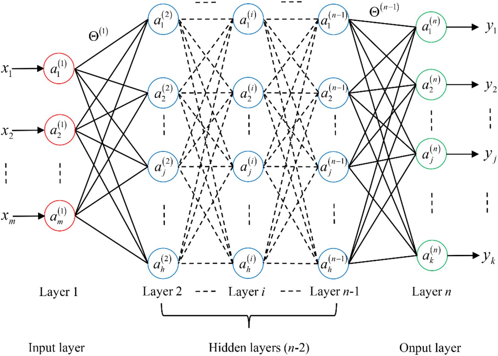
Figure 5. Diagram of an n-layer neural network. In this neural network, i is the number of layers and j is the number of units in each layer. x1,x2,…,xm represent input units, while y1,y2,…,yk represent output units. represents the j-th activation unit in the i-layer, which is responsible for mapping the input of a neuron to the output. Θ(i) represents the weight from the i-th layer to the i+1-th layer, whose function is to adjust the proportion of each input value before entering the activation function. Furthermore, we sometimes add a bias unit to each layer to reduce the error of the output value.
The core of SVMs is to find the one hyperplane with the largest margin out of many hyperplanes that divide the training set (Cortes and Vapnik, 1995). The mathematical representation is:
where mf is the number of features, ϕ(x) is the eigenvector after x mapping and f(x) = ωTϕ(x) + b is the mathematical representation of the hyperplane.
The final performance of SVMs is directly determined by the kernel function (Crammer and Singer, 2002):
where αL is the Lagrange multiplier and κ(x,xi) = ϕT(xi)ϕ(x) is the kernel. Commonly used kernel functions are shown in Table 3.
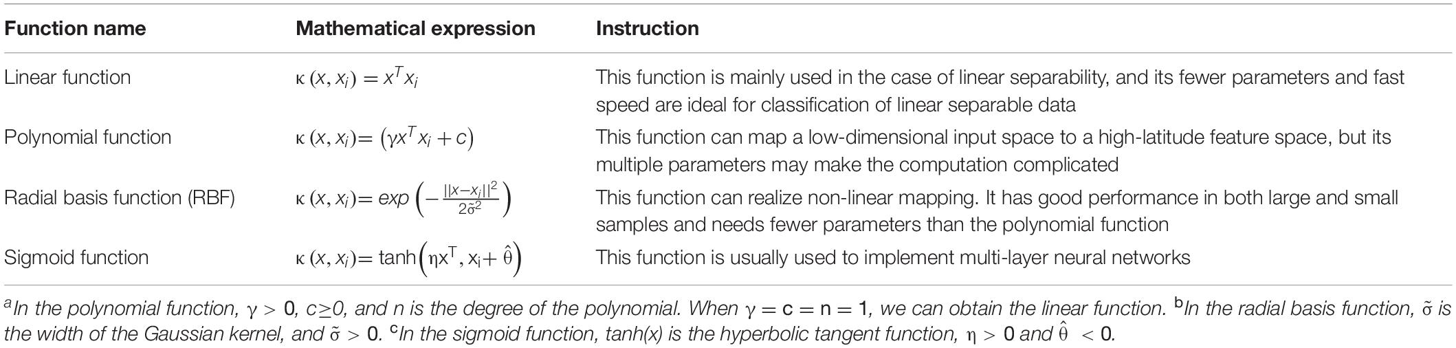
Table 3. List of commonly used kernel functions.
The linear function has the advantage of fewer parameters and fast speed but can be used only in the case of linear separability. Although the polynomial function can map a low-dimensional input space to a high-latitude feature space, its multiple parameters may make the computation complicated. In contrast, the radial basis function (RBF) has good performance in both large and small samples and requires fewer parameters than the polynomial function. Therefore, the RBF is widely used in SVMs.
Unsupervised Learning
The major task of unsupervised learning is data clustering. Clustering is one of the data mining techniques in which data are divided into groups of similar and dissimilar objects by using the intrinsic relations between data (Saroj and Kavita, 2016).
K-means clustering is the most basic clustering algorithm. The idea is to measure the similarity between different data objects by using the Euclidean distance. The similarity is inversely proportional to the Euclidean distance between different data objects. If the similarity between the data objects is greater, the Euclidean distance is smaller.
The local optimal solution of the K-means algorithm (yi) is the minimum value of the sum of distances between all data points and their associated cluster centroids. It can be calculated as:
where mt is the total number of samples, k is the total number of clusters, Cj is the j-th cluster, uj is the cluster centroid of Cj and nj is the number of samples in Cj. The workflow of the K-means clustering algorithm is shown in Figure 6.
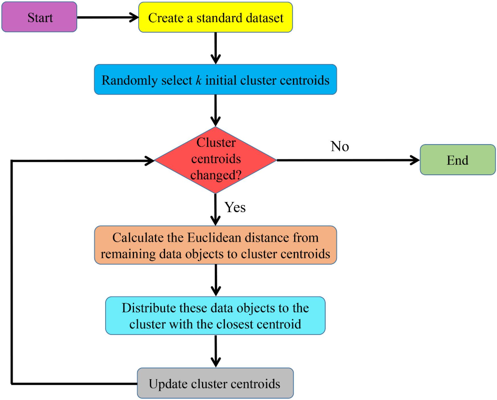
Figure 6. The workflow of the K-means clustering algorithm. This algorithm needs to select k initial cluster centroids in advance. Then, the positions of cluster centroids are continuously updated according to the similarity between data objects and these positions. When updated cluster centroids no longer change or the objective function converges, the iteration ends, and the final result can be obtained.
The K-means algorithm is very efficient when dealing with a large dataset. However, there are typically still two disadvantages: sensitivity to the initial value and ease of falling into a local optimal solution (Hung et al., 2013).
In short, these basic algorithms of ML do not have absolutely clear scopes of application. We should choose a relatively appropriate algorithm according to specific problems.
Applications of Machine Learning in Induced Seismicity
Incorporating novel ML into traditional seismological methods could provide great benefit. Kong et al. (2018) reviewed several current applications of ML in seismology, including earthquake detection and phase picking, real-time earthquake early warning, ground-motion prediction, seismic tomography and earthquake geodesy, etc. However, these applications are mainly focused on natural earthquakes. Since in the induced seismicity context one has to establish a causative connection between the human activities and detected seismicity, studying induced seismicity needs more data than studying natural earthquakes, especially operational data, which reflect the information of industrial activities. Unfortunately, some operational data are hardly available to the public. This is the main obstacle to applying ML to induced seismicity. For this reason, the current application of ML in induced seismicity is mainly focused on the laboratory study of mechanism, while the preliminary field applications are relatively rare.
Laboratory Study of the Mechanism
The seismogenic mechanism of induced seismicity is absolutely vital for managing induced seismicity, and laboratory rock testing is an important means to understand its mechanism. Energy stored in rocks is released in the form of elastic waves, which are called acoustic emissions (AEs), during micro-crack initiation, propagation and connection in the laboratory (Lei et al., 2003; Liu et al., 2019; Yue et al., 2019). The phenomena of micro-seismicity at the field scale and AEs in the laboratory are similar in nature (Sarout et al., 2017), and high-quality microseismic observations can effectively improve the statistical models that forecast expected seismic event magnitudes (Clarke et al., 2019). Therefore, the accurate identification and location of rock AE signals in the laboratory is of great significance for the study of induced seismicity.
Liu et al. (2015) used wavelet transform and ANNs to study the AE characteristics of different rock specimens during fracture under uniaxial compression. They created an efficient way to identify rock types and noise based on wavelet transform and ANNs. Rouet-Leduc et al. (2017) and Hulbert et al. (2018) applied the ML method to identify AE signals from fault shear experiments and AE signals before both slow and fast slip modes. It was found that ML could not only effectively identify AE signals that were previously considered to represent low-amplitude fault zones but also successfully predict the timing and duration of laboratory earthquakes. Rock fracture and blast events have similar waveform characteristics, and they are always mixed together. To effectively distinguish the AE signals of rocks from environmental noise and other signals, Zhou et al. (2018) proposed a new method based on signal complexity analysis and ML. This method did not seek waveform parameters of detected signals and could classify rock fracture and blast signals automatically based on the self-learning capacity of back propagation neural networks (BPNNs). On this basis, (Zhou et al., 2019a, b, 2020) further proposed an improved joint method based on discrete wavelet transform, modified energy ratio and Akaike information criterion (AIC) pickers, which effectively overcame the interference of spike noise and channel crosstalk and greatly improved the accuracy of automatic method for picking onset time of AE signals.
These results indicate that using ML method can capture more comprehensive and accurate rock fracture information at the laboratory scale, which can help us deepen understanding of the mechanism and further improve the physical and statistical models of induce seismicity.
Preliminary Exploration and Application in the Field
For seismicity induced by EGS exploitation, Holtzman et al. (2018) studied various small earthquake events in the Geysers geothermal field using the ML method, indicating that it could reveal the time-dependent spectral characteristics of seismicity signals and identify changes in the faulting process. In response to a large number of induced earthquakes in Oklahoma since 2009, Hincks et al. (2018) developed an advanced Bayesian network to model joint conditional dependencies among spatial, operational and seismic parameters, indicating that the injection depth was closely related to the release of the seismic moment. The model they proposed proved the feasibility and superiority of using ML to establish the mapping relationship between operational parameters and seismic information.
Using Machine Learning Method to Improve Adaptive Traffic Light System
The importance of TLS for managing induced seismic risks has been illustrated in section “Traffic Light System for Safe Production.” One of the ways to improve TLS is to develop a risk-based adaptive TLS. The work of Mignan et al. (2017) has great reference value. They used statistical and actuarial approaches to improve the current prediction model (mentioned in section “Traffic Light System for Safe Production”) of induced seismic activity, and further proposed an adaptive traffic light system (called ATLS) that can reflect the mapping relationship between earthquake magnitude and risk.
In this ATLS, the threshold magnitude is selected as the decision variable. They put forward a method to calculate the threshold magnitude so that it can be updated in time with the change of the planned injection scheme.
where Mth is the threshold magnitude in ATLS, and the meaning of other parameters can be found in Eq. (5) and Eq. (6).
Based on it, they then defined the ATLS as the operational threshold Mth at which the injection was stopped in order to meet the safety target, and thus obtained the following system of equations [for the meaning of the symbols, please see Eq. (5) and Eq. (6)]:
In Eq. (14), the first equation represents the situation of production safety. The probability that the magnitude exceeds the threshold is much less than 1 (i.e., Y ≪ 1), and Mth≈Msaf can be obtained according to Eq. (13). The second equation represents the first time during the production process that the magnitude exceeds the threshold (i.e., Y = 1). At this point, the injection should be stopped immediately (t = tshut−in, ), and Mth = Msaf can be obtained according to Eq. (13). In particular, m0 in Eq. (5) can be replaced by Mth to consider induced seismic activity in the post-injection phase.
The quantitative risk-based ATLS they proposed is a suite of simple closed-form expressions, with the advantages of high transparency and fast execution speed, which can provide the operator with the greatest chance of success. It is important to note, however, that the data set used to generate ATLS is relatively small (only data from 6 underground reservoir stimulation experiments were used for analysis), so its application scope needs further testing, although in principle its adoption would make any project in compliance with the safety threshold whatever the response of the underground.
The present study points the way for developing risk-based adaptive TLS and also illustrates that a large number of operational data are needed to improve TLS. In terms of big data processing, ML method is superior to traditional actuarial approach. Using ML methods to further improve the adaptive TLS has attractive potential.
Basic Framework
In order to solve the shortcomings of the ATLS proposed by Mignan et al. (2017), this section describes a basic framework for further improving the adaptive TLS by using ML method. Through the training and learning of a large number of samples, a proxy model that reflects the complex non-linear relationship between threshold magnitude and operating parameters can be obtained. The implementation process of the basic framework is shown in Figure 7.
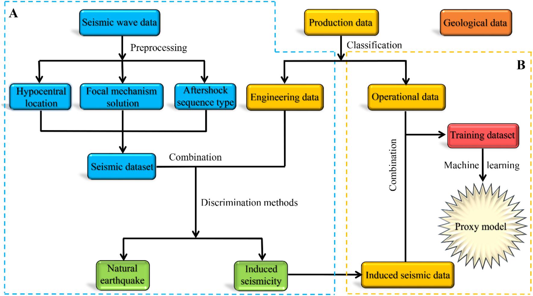
Figure 7. Flowchart for using machine learning methods to improve the adaptive TLS. (A) Identify induced seismicity and (B) Determine the proxy model.
The establishment of the proxy model requires sufficient geological, seismic and production data. Geological data include information such as geomechanical and hydraulic parameters, which can be obtained through geological exploration. Seismic data mainly contain waveform information that can be acquired by monitoring at nearby seismic stations. Production data can be divided into engineering data and operational data. The engineering data mainly include drilling information, such as drilling time, drilling position, drilling depth and the number of wells, while the operational data reflect the information about injection operational parameters, such as wellhead pressure, total injection amount, injection speed and injection position.
For a specific study region, the local geological data should be acquired in advance, which include geomechanical and hydraulic parameters. Next, we must collect seismicity wave data and the engineering dataset in this region over a relatively long period of time (e.g., 5 or 10 years) to ensure that the dataset is comparatively complete. It should be noted that the seismic wave data are mixtures of natural and induced earthquake information (i.e., unlabelled), while the engineering dataset contains some previously known drilling information (i.e., labeled). Then, the original data for earthquake events, including hypocentral location, focal mechanism solution and aftershock sequence type analysis, need to be pre-processed to obtain the seismic dataset. The seismic dataset and the engineering dataset are combined, and methods mentioned in section “Discrimination of Natural and Induced Seismicity” can be used to distinguish the induced seismic events, as shown in Figure 7A. There are some relations between induced seismicity data and engineering data. Finally, we can form a training dataset based on the relationship between the induced seismicity data and operational data. These data are taken as prior knowledge for ML. Since both induced seismicity data and operational data are labeled, we can use the supervised learning methods mentioned in section “Supervised Learning” to train this dataset and further fit a proxy model, as shown in Figure 7B.
Additionally, to ensure the generalization ability of the training model, over-fitting should be mitigated to the greatest extent. To improve the algorithms, we can divide the original dataset into three parts: training dataset, validation dataset and testing dataset before training. According to the performance of the training model on the cross-validation dataset and testing dataset, the generalization ability of this proxy model could be roughly determined (Santos et al., 2018).
Similar Cases
In this section, the theoretical feasibility of the basic framework will be demonstrated with some real cases. However, as mentioned in section “Applications of Machine Learning in Induced Seismicity,” there is almost no public report on the use of ML for injection-induced seismic risk management. To overcome this difficulty, we select some similar cases that use ML to manage reservoir-induced seismicity (RIS). At present, the application of ML in reservoir induced earthquake is mainly reflected in the prediction of earthquake magnitude based on reservoir parameters, which is very similar to the real-time evaluation of threshold magnitude in TLS.
Samui and Kim (2013) used SVM and Gaussian process regression (GPR) models in ML to predict the magnitude of RIS based on reservoir properties. At first, they collected information from 30 worldwide historical cases of RIS into dataset. These data were taken as prior knowledge for SVM and GPR models. Reservoir depth HR, reservoir capacity VR, reservoir surface SR and earthquake magnitude M were suggested to be main influential factors of RIS. In that study, they used the comprehensive parameter E to characterize the three elements (i.e., HR, VR, SR) of reservoir size, which could be expressed as E = SRHR/VR (Baoqi, 1990). These parameters could well reflect the internal and exterior causes of RIS. Then, to develop the SVM and GPR, they divided the dataset into two types: the training dataset (containing information about 24 reservoirs) and the testing dataset (containing information about 6 reservoirs). The comprehensive parameter E and the reservoir depth HR were used as input variables, while the earthquake magnitude M was output. Finally, through learning process by SVM and GPR models, the complex mapping relationship between RIS magnitude and its influence factors was established, respectively. Thus the magnitude could be controlled by adjusting the input parameters in the relationship.
It is worth noting that the correlation coefficient (R) value is the criterion for determining the success of the learning process. The closer R is to 1, the more accurate the mapping relationship (overlearning needs to be excluded). For SVM model, the penalty coefficient , the error insensitive zone and the radial basis function width should be determined. As for GPR model, the design values that need to be determined are the Gaussian noise and the radial basis function width .
Based on those studies, Samui and Kim (2014) further tested the feasibility of least square support vector machine (LSSVM) and relevance vector machine (RVM) in predicting RIS magnitude and compared the results with ANN and linear regression models. They found that the LSSVM and RVM models were more efficient and effective. Furthermore, Su (2008) also used the GPR model to predict the magnitude of RIS in western China. They considered more impact parameters in learning process, including reservoir depth, tectonic stress, lithologic character, activity background of seismicity, activity of fault, development degree of geology structure plane, connectivity between geology structure plane and reservoir water, and development degree of karst, etc. Their method has been applied to control RIS magnitude at the Three Gorges Reservoir in China. Although these achievements are limited to RIS, it provides ideas and confidence for using ML to manage the risk of injection-induced seismicity also for other kinds of activities.
Some Statements
(1) Decision variable: Since the basic framework is based on the results of Mignan et al. (2017), it takes the threshold magnitude as the decision variable for induced seismic risk control. If PGV or other parameters are selected as decision variables, they must be converted to the corresponding magnitude.
(2) Application scope: The operational parameters mentioned in the basic framework mainly involve some fluid injection information. Therefore, it is mainly applicable to injection-induced seismicity, including wastewater reinjection, hydraulic fracturing and geothermal energy exploitation, etc. Notably, for different activities, it is necessary to collect corresponding key parameters according to the characteristics of the activities and take these parameters as the prior knowledge for ML training. The combination of ML methods with specific TLS models implemented for different activities is very important.
(3) Post-injection phase: The basic framework can also consider the post-injection phase. To do this, we need to expand the time window to a period of time after shut-in and collect the data. Then, the data before and after shut-in are trained to establish their proxy models, respectively.
(4) Main challenges: The complete collection of relevant data is a major challenge, because some production data is hardly available to the public. In addition, the efficient processing of large amounts of data is also a problem faced by ML.
Conclusion
This paper provides an overview of current research progress of induced seismicity related to fluid injection, and proposes a basic framework of using ML method to improve the adaptive TLS. The implementation process of the framework has been described in detail, and its feasibility and rationality have also been demonstrated by some cases related to reservoir-induced seismicity.
The proposed framework uses the threshold magnitude as the decision variable and can also consider the post-injection phase after shut-in. Compared with the statistical and actuarial approaches, the proxy model based on ML training with a large amount of data can more comprehensively reflect the complex relationship between operational and seismic parameters. Moreover, it can be applied to various injection-induced earthquakes by collecting characteristic data of different activities. However, the complete collection of relevant data is the primary challenge.
We hope that this basic framework can provide valuable references for developing the risk-based adaptive TLS models in the future.
Author Contributions
QL designed the research project. MH and XL wrote the manuscript. All authors performed the research, analyzed the results, and finally approved the manuscript.
Funding
This work was partially supported by the National Natural Science Foundation of China (Grant Nos. 41872210 and 41902297) and Open Research Fund of State Key Laboratory of Geomechanics and Geotechnical Engineering, Institute of Rock and Soil Mechanics, Chinese Academy of Sciences (Grant No. Z017006).
Conflict of Interest
The authors declare that the research was conducted in the absence of any commercial or financial relationships that could be construed as a potential conflict of interest.
Acknowledgments
We would like to thank all the reviewers for their insightful and constructive comments on the manuscript, as these comments led us to a real improvement of the current work.
Abbreviations
AE, acoustic emission; AI, artificial intelligence; AIC, Akaike information criterion; ANN, artificial neural network; ATLS, adaptive traffic light system; BPNN, back propagation neural network; CLVD, compensated linear vector dipole; CNY, Chinese Yuan; CO2, carbon dioxide; DC, double-couple; EGS, enhanced geothermal system; ETAS, epidemic-type aftershock sequence; FLAC, fast Lagrangian analysis of continua; GPR, Gaussian process regression; Graviquakes, fluid removal from a stratigraphic reservoir that can cause normal faults-related earthquakes; ISO, isotropic; LSSVM, least square support vector machine; ML, machine learning; MT, moment tensor; PGV, peak ground velocity; RBF, radial basis function; RIS, reservoir-induced seismicity; RVM, relevance vector machine; SVM, support vector machine; THM, thermal-hydrological-mechanical; TLS, traffic light system; TOUGH, transport of unsaturated groundwater and heat; US, the United States.
References
Afonso, L., Vidal, A., Kuroda, M., Falcao, A. X., and Papa, J. P. (2016). “learning to classify seismic images with deep optimum-path forest,” in Proceedings of the 2016 29th SIBGRAPI Conference on Graphics, Patterns and Images (SIBGRAPI), São Paulo.
Aghajanyan, A. (2017). “Softtarget regularization: an effective technique to reduce over-fitting in neural networks,” in Proceedings of the 2017 3rd IEEE International Conference on Cybernetics (CYBCONF), Piscataway, NJ.
Albano, M., Barba, S., Tarabusi, G., Saroli, M., and Stramondo, S. (2017). Discriminating between natural and anthropogenic earthquakes: insights from the Emilia Romagna (Italy) 2012 seismic sequence. Sci. Rep. 7:282. doi: 10.1038/s41598-017-00379-2
Alcoverro, J. (2003). The effective stress principle. Math. Comput. Model. 37, 457–467. doi: 10.1016/s0895-7177(03)00038-4
Amini, A., and Eberhardt, E. (2019). Influence of tectonic stress regime on the magnitude distribution of induced seismicity events related to hydraulic fracturing. J. Petrol. Sci. Eng. 182:106284. doi: 10.1016/j.petrol.2019.106284
Asim, K. M., Martínez-lvarez, F., Basit, A., and Iqbal, T. (2016). Earthquake magnitude prediction in Hindukush region using machine learning techniques. Nat. Haz. 85, 471–486. doi: 10.1007/s11069-016-2579-3
Baisch, S., Koch, C., and Muntendam-Bos, A. (2019). Traffic light systems: to what extent can induced seismicity be controlled? Seismol. Res. Lett. 90, 1145–1154. doi: 10.1785/0220180337
Bao, X., and Eaton, D. W. (2016). Fault activation by hydraulic fracturing in western Canada. Science 354, 1406–1409. doi: 10.1126/science.aag2583
Baoqi, C. (1990). Preliminary study on the prediction of reservoir earthquakes. Gerlands Beiträge Zur Geophysik 99, 407–424.
Bialas, J., Oommen, T., Rebbapragada, U., and Levin, E. (2016). Object-based classification of earthquake damage from high-resolution optical imagery using machine learning. J. Appl. Remote Sens. 10:e036025.
Bommer, J. J., Oates, S., Cepeda, J. M., Lindholm, C., Bird, J., Torres, R., et al. (2006). Control of hazard due to seismicity induced by a hot fractured rock geothermal project. Eng. Geol. 83, 287–306. doi: 10.1016/j.enggeo.2005.11.002
Boyd, O. S., Dreger, D. S., Gritto, R., and Garcia, J. (2018). analysis of seismic moment tensors and in-situ stress during enhanced geothermal system development at the geysers geothermal field, California. Geophys. J. Intern. 215, 1483–1500. doi: 10.1093/gji/ggy326
Braun, T., Danesi, S., and Morelli, A. (2020). Application of monitoring guidelines to induced seismicity in Italy. J. Seismol. doi: 10.1007/s10950-019-09901-7 [Epub ahead of print].
Cawley, G. C., and Talbot, N. L. (2007). Preventing over-fitting during model selection via Bayesian regularisation of the hyper-parameters. J. Mach. Learn. Res. 8, 841–861.
Cesca, S., Rohr, A., and Dahm, T. (2012). Discrimination of induced seismicity by full moment tensor inversion and decomposition. J. Seismol. 17, 147–163. doi: 10.1007/s10950-012-9305-8
Clarke, H., Verdon, J. P., Kettlety, T., Baird, A. F., and Kendall, J. M. (2019). Real-Time imaging, forecasting, and management of human-induced seismicity at preston new road, lancashire, England. Seismol. Res. Lett. 90, 1902–1915.
Clerc, F., Harrington, R. M., Liu, Y., and Gu, Y. J. (2016). Stress drop estimates and hypocenter relocations of induced seismicity near Crooked Lake, Alberta. Geophysical Research Letters 43, 6942–6951. doi: 10.1002/2016gl069800
Corbi, F., Sandri, L., Bedford, J., Funiciello, F., Brizzi, S., Rosenau, M., et al. (2019). Machine learning can predict the timing and size of analog earthquakes. Geophys. Res. Lett. 46, 1303–1311. doi: 10.1029/2018gl081251
Crammer, K., and Singer, Y. (2002). On the algorithmic implementation of multiclass kernel–based vector machines. J. Mach. Learn. Res. 2, 265–292.
Currie, B. S., Free, J. C., Brudzinski, M. R., Leveridge, M., and Skoumal, R. J. (2018). Seismicity induced by wastewater injection in washington county, ohio: influence of preexisting structure, regional stress regime, and well operations. J. Geophys. Res. Solid Earth 123, 4123–4140. doi: 10.1002/2017jb015297
Dahm, T., Becker, D., Bischoff, M., Cesca, S., Dost, B., Fritschen, R., et al. (2012). Recommendation for the discrimination of human-related and natural seismicity. J. Seismol. 17, 197–202. doi: 10.1007/s10950-012-9295-6
Dahm, T., Cesca, S., Hainzl, S., Braun, T., and Krüger, F. (2015). Discrimination between induced, triggered, and natural earthquakes close to hydrocarbon reservoirs: a probabilistic approach based on the modeling of depletion-induced stress changes and seismological source parameters. J. Geophys. Res. Solid Earth 120, 2491–2509. doi: 10.1002/2014jb011778
Davis, S. D., and Frohlich, C. (1993). Did (or will) fluid injection cause earthquakes — Criteria for a rational assessment. Seismol. Res. Lett. 64, 207–224. doi: 10.1785/gssrl.64.3-4.207
DeVries, P. M. R., Viegas, F., Wattenberg, M., and Meade, B. J. (2018). Deep learning of aftershock patterns following? large earthquakes. Nature 560, 632–634. doi: 10.1038/s41586-018-0438-y
Doglioni, C. (2018). A classification of induced seismicity. Geosci. Front. 9, 1903–1909. doi: 10.1016/j.gsf.2017.11.015
Eaton, D. W., and Igonin, N. (2018). What controls the maximum magnitude of injection-induced earthquakes? Lead. Edge 37, 135–140. doi: 10.1190/tle37020135.1
Ellsworth, W. L. (2013). Injection-induced earthquakes. Science 341:1225942. doi: 10.1126/science.1225942
Ellsworth, W. L., Giardini, D., Townend, J., Ge, S., and Shimamoto, T. (2019). Triggering of the Pohang, Korea, Earthquake (Mw 5.5) by enhanced geothermal system stimulation. Seismol. Res. Lett. 90, 1844–1858.
Evans, D. M. (1966). The Denver area earthquakes and the rocky mountain arsenal disposal well. Mount. Geol. 3, 23–26.
Figueiredo, B., Tsang, C.-F., Rutqvist, J., Bensabat, J., and Niemi, A. (2015). Coupled hydro-mechanical processes and fault reactivation induced by CO2 Injection in a three-layer storage formation. Intern. J. Greenhouse Gas Control 39, 432–448. doi: 10.1016/j.ijggc.2015.06.008
Folger, P., and Tiemann, M. (2017). Human-Induced Earthquakes From Deep-Well Injection: A Brief Overview. Washington, DC: Congressional Research Service.
Foulger, G. R., Wilson, M. P., Gluyas, J. G., Julian, B. R., and Davies, R. J. (2018). Global review of human-induced earthquakes. Earth Sci. Rev. 178, 438–514. doi: 10.1016/j.earscirev.2017.07.008
Frank, J., Rebbapragada, U., Bialas, J., Oommen, T., and Havens, T. (2017). Effect of label noise on the machine-learned classification of earthquake damage. Remote Sens. 9:803. doi: 10.3390/rs9080803
Franklin, J. (2005). The elements of statistical learning data mining, inference, and prediction. Math. Intellig. 27, 83–85. doi: 10.1007/bf02985802
Galis, M., Ampuero, J. P., Mai, P. M., and Cappa, F. (2017). Induced seismicity provides insight into why earthquake ruptures stop. Sci. Adv. 3:7528.
Gaucher, E., Schoenball, M., Heidbach, O., Zang, A., Fokker, P. A., Van Wees, J. D., et al. (2015). Induced seismicity in geothermal reservoirs: a review of forecasting approaches. Renew. Sustain. Energy Rev. 52, 1473–1490. doi: 10.1016/j.rser.2015.08.026
Ghofrani, H., and Atkinson, G. M. (2016). A preliminary statistical model for hydraulic fracture-induced seismicity in the western canada sedimentary Basin. Geophys. Res. Lett. 43:10164.
Giardini, D. (2009). Geothermal quake risks must be faced. Nature 462, 848–849. doi: 10.1038/462848a
Gibson, G., and Sandiford, M. (2013). Seismicity & Induced Earthquakes. Background Paper to NSW Chief Scientist and Engineer (OCSE). Melbourne: University of Melbourne.
Gilbert, F. (1971). Excitation of the normal modes of the earth by earthquake sources. Geophys. J. Intern. 22, 223–226. doi: 10.1111/j.1365-246x.1971.tb03593.x
Goertz-Allmann, B. P., Gibbons, S. J., Oye, V., Bauer, R., and Will, R. (2017a). Characterization of induced seismicity patterns derived from internal structure in event clusters. J. Geophys. Res. Solid Earth 122, 3875–3894. doi: 10.1002/2016jb013731
Goertz-Allmann, B. P., Oye, V., Gibbons, S. J., and Bauer, R. (2017b). Geomechanical monitoring of CO2 storage reservoirs with microseismicity. Energy Proc. 114, 3937–3947. doi: 10.1016/j.egypro.2017.03.1525
Goertz-Allmann, B. P., Kühn, D., Oye, V., Bohloli, B., and Aker, E. (2014). Combining microseismic and geomechanical observations to interpret storage integrity at the in Salah CCS site. Geophys. J. Intern. 198, 447–461. doi: 10.1093/gji/ggu010
Grasso, J. R., and Wittlinger, G. (1990). Ten years of seismic monitoring over a gas field. Bull. Seismol. Soc. Am. 80, 450–473.
Grigoli, F., Cesca, S., Priolo, E., Rinaldi, A. P., Clinton, J. F., Stabile, T. A., et al. (2017). Current challenges in monitoring, discrimination, and management of induced seismicity related to underground industrial activities: a European perspective. Rev. Geophys. 55, 310–340. doi: 10.1002/2016rg000542
Guglielmi, Y., Cappa, F., Avouac, J. P., Henry, P., and Elsworth, D. (2015). Seismicity triggered by fluid injection-induced aseismic slip. Science 348, 1224–1226. doi: 10.1126/science.aab0476
Hainzl, S., and Ogata, Y. (2005). Detecting fluid signals in seismicity data through statistical earthquake modeling. J. Geophys. Res.Solid Earth 110: B05S07.
Healy, J. H., Rubey, W. W., Griggs, D. T., and Raleigh, C. B. (1968). the denver earthquakes. Science 161, 1301–1310. doi: 10.1126/science.161.3848.1301
Herber, R., and de Jager, J. (2014). Geoperspective oil and gas in the Netherlands – is there a future? Nether. J. Geosci. Geol. Mijnb. 89, 91–107. doi: 10.1017/s001677460000072x
Hincks, T., Aspinall, W., Cooke, R., and Gernon, T. (2018). Oklahoma’s induced seismicity strongly linked to wastewater injection depth. Science 359, 1251–1255. doi: 10.1126/science.aap7911
Hinton, G. E., and Salakhutdinov, R. R. (2006). Reducing the dimensionality of data with neural networks. Science 313, 504–507. doi: 10.1126/science.1127647
Hofmann, H., Zimmermann, G., Zang, A., and Min, K. B. (2018). Cyclic soft stimulation (CSS): a new fluid injection protocol and traffic light system to mitigate seismic risks of hydraulic stimulation treatments. Geotherm. Energy 6:27.
Holtzman, B. K., Paté, A., Paisley, J., Waldhauser, F., and Repetto, D. (2018). Machine learning reveals cyclic changes in seismic source spectra in Geysers geothermal field. Sci. Adv. 4:eaao2929. doi: 10.1126/sciadv.aao2929
Hsieh, P. A., and Bredehoeft, J. D. (1981). A reservoir analysis of the denver earthquakes: a case of induced seismicity. J. Geophys. Res. Solid Earth 86, 903–920. doi: 10.1029/jb086ib02p00903
Hulbert, C., Rouet-Leduc, B., Johnson, P. A., Ren, C. X., Rivière, J., Bolton, D. C., et al. (2018). Similarity of fast and slow earthquakes illuminated by machine learning. Nat. Geosci. 12, 69–74. doi: 10.1038/s41561-018-0272-8
Hung, C.-H., Chiou, H.-M., and Yang, W.-N. (2013). Candidate groups search for K-harmonic means data clustering. Appl. Math. Model. 37, 10123–10128. doi: 10.1016/j.apm.2013.05.052
Jechumtálová, Z., and Bulant, P. (2014). Effects of 1-D versus 3-D velocity models on moment tensor inversion in the Dobrá Voda area in the Little Carpathians region, Slovakia. J. Seismol. 18, 511–531. doi: 10.1007/s10950-014-9423-6
Kim, H. S., Sun, C. G., and Cho, H. I. (2018). Geospatial assessment of the post-earthquake hazard of the 2017 Pohang earthquake considering seismic site effects. ISPRS Intern. J. Geo Inform. 7:375. doi: 10.3390/ijgi7090375
Kong, Q., Trugman, D. T., Ross, Z. E., Bianco, M. J., Meade, B. J., and Gerstoft, P. (2018). Machine learning in seismology: turning data into insights. Seismol. Res. Lett. 90, 3–14. doi: 10.1785/0220180259
Lee, K. K., Ellsworth, W. L., Giardini, D., Townend, J., Ge, S., Shimamoto, T., et al. (2019). Managing injection-induced seismic risks. Science 364, 730–732. doi: 10.1126/science.aax1878
Lei, X., Huang, D., Su, J., Jiang, G., Wang, X., Wang, H., et al. (2017). Fault reactivation and earthquakes with magnitudes of up to Mw4.7 induced by shale-gas hydraulic fracturing in Sichuan Basin, China. Sci. Rep. 7:7971.
Lei, X., Kusunose, K., Satoh, T., and Nishizawa, O. (2003). The hierarchical rupture process of a fault: an experimental study. Phys. Earth Planet. Inter. 137, 213–228. doi: 10.1016/s0031-9201(03)00016-5
Lei, X., Ma, S., Chen, W., Pang, C., Zeng, J., and Jiang, B. (2013). A detailed view of the injection-induced seismicity in a natural gas reservoir in Zigong, southwestern Sichuan Basin, China. J. Geophys. Res. Solid Earth 118, 4296–4311. doi: 10.1002/jgrb.50310
Lei, X., Wang, Z., and Su, J. (2019). The december 2018 ML5.7 and January 2019 ML5.3 earthquakes in South Sichuan basin induced by shale gas hydraulic fracturing. Seismol. Res. Lett. 90, 1099–1110. doi: 10.1785/0220190029
Lei, X., Yu, G., Ma, S., Wen, X., and Wang, Q. (2008). Earthquakes induced by water injection at 3 km depth within the Rongchang gas field, Chongqing, China. J. Geophys. Res. Solid Earth 113:B10310.
Liu, X., Liang, Z., Zhang, Y., Wu, X., and Liao, Z. (2015). Acoustic emission signal recognition of different rocks using wavelet transform and artificial neural network. Shock Vibrat. 2015, 1–14. doi: 10.1155/2015/846308
Liu, X., Liu, Q., Liu, B., and Liu, Q. (2019). Acoustic emission characteristics of pre-cracked specimens under biaxial compression. J. Geophys. Eng. 16, 1164–1177. doi: 10.1093/jge/gxz087
Love, B. C. (2002). Comparing supervised and unsupervised category learning. Psychon. Bull. Rev. 9, 829–835. doi: 10.3758/bf03196342
Lubbers, N., Bolton, D. C., Mohd-Yusof, J., Marone, C., Barros, K., and Johnson, P. A. (2018). Earthquake catalog-based machine learning identification of laboratory fault states and the effects of magnitude of completeness. Geophys. Res. Lett. 45, 269–213.
Macdonald, J., Backé, G., King, R., Holford, S., and Hillis, R. (2012). Geomechanical modelling of fault reactivation in the Ceduna Sub-basin, Bight Basin, Australia. Geol. Soc. Lond. Spec. Public. 367, 71–89. doi: 10.1144/sp367.6
Majer, E. L., and Peterson, J. E. (2007). The impact of injection on seismicity at the geysers, California geothermal field. Intern. J. Rock Mech. Min. Sci. 44, 1079–1090. doi: 10.1016/j.ijrmms.2007.07.023
Martínez-Garzón, P., Kwiatek, G., Bohnhoff, M., and Dresen, G. (2016). Impact of fluid injection on fracture reactivation at the geysers geothermal field. J. Geophys. Res. Solid Earth 121, 7432–7449. doi: 10.1002/2016jb013137
McCulloch, W. S., and Pitts, W. (1943). A logical calculus of the ideas immanent in nervous activity. Bull. Math. Biophys. 5, 115–133. doi: 10.1007/bf02478259
McGarr, A. (2014). Maximum magnitude earthquakes induced by fluid injection. J. Geophys. Res. Solid Earth 119, 1008–1019. doi: 10.1002/2013jb010597
McGarr, A., Simpson, D., and Seeber, L. (2002). 40 Case histories of induced and triggered seismicity. Intern. Handb. Earthq. Eng. Seismol. 81, 647–661. doi: 10.1016/s0074-6142(02)80243-1
Mignan, A., Broccardo, M., Wiemer, S., and Giardini, D. (2017). Induced seismicity closed-form traffic light system for actuarial decision-making during deep fluid injections. Sci. Rep. 7, 1–10.
Mnih, V., Kavukcuoglu, K., Silver, D., Rusu, A. A., Veness, J., Bellemare, M. G., et al. (2015). Human-level control through deep reinforcement learning. Nature 518, 529–533.
National Research Council (2013). Induced Seismicity Potential In Energy Technologies. Washington, DC: National Academies Press.
Nicol, A., Carne, R., Gerstenberger, M., and Christophersen, A. (2011). Induced seismicity and its implications for CO2 storage risk. Energy Proc. 4, 3699–3706. doi: 10.1016/j.egypro.2011.02.302
Pan, S. J., and Yang, Q. A. (2010). A survey on transfer learning. IEEE Trans. Knowl. Data Eng. 22, 1345–1359.
Passarelli, L., Maccaferri, F., Rivalta, E., Dahm, T., and Abebe Boku, E. (2012). A probabilistic approach for the classification of earthquakes as ‘triggered’ or ‘not triggered’. J. Seismol. 17, 165–187. doi: 10.1007/s10950-012-9289-4
Pratt, W. E., and Johnson, D. W. (1926). Local Subsidence of the Goose Creek Oil Field. J. Geol. 34, 577–590. doi: 10.1086/623352
Rajguru, G., Bhadauria, Y. S., and Mukhopadhyay, S. (2018). “Estimation of earthquake source parameters using machine learning techniques,” in Proceedings of the International Conference on Computing, Communication and Networking Technologies, 9th IEEE, New York, NY.
Rinaldi, A. P., and Nespoli, M. (2017). TOUGH2-seed: a coupled fluid flow and mechanical-stochastic approach to model injection-induced seismicity. Comput. Geosci. 108, 86–97. doi: 10.1016/j.cageo.2016.12.003
Rouet-Leduc, B., Hulbert, C., Lubbers, N., Barros, K., Humphreys, C. J., and Johnson, P. A. (2017). Machine learning predicts laboratory earthquakes. Geophys. Res. Lett. 44, 9276–9282. doi: 10.1002/2017gl074677
Rumelhart, D. E., Hinton, G. E., and Williams, R. J. (1986). Learning representations by back-propagating errors. Nature 323, 533–536. doi: 10.1038/323533a0
Rutqvist, J., Rinaldi, A. P., Cappa, F., and Moridis, G. J. (2015). Modeling of fault activation and seismicity by injection directly into a fault zone associated with hydraulic fracturing of shale-gas reservoirs. J. Petrol. Sci. Eng. 127, 377–386. doi: 10.1016/j.petrol.2015.01.019
Rutqvist, J., Vasco, D. W., and Myer, L. (2010). Coupled reservoir-geomechanical analysis of CO2 injection and ground deformations at In Salah, Algeria. Intern. J. Greenhouse Gas Control 4, 225–230. doi: 10.1016/j.ijggc.2009.10.017
Samui, P., and Kim, D. (2013). Determination of reservoir induced earthquake using support vector machine and gaussian process regression. Appl. Geophys. 10, 229–234. doi: 10.1007/s11770-013-0381-5
Samui, P., and Kim, D. (2014). Applicability of artificial intelligence to reservoir induced earthquakes. Acta Geophys. 62, 608–619. doi: 10.2478/s11600-014-0201-1
Santos, M. S., Soares, J. P., Abreu, P. H., Araujo, H., and Santos, J. (2018). “Cross-validation for imbalanced datasets: avoiding overoptimistic and overfitting approaches [research frontier],” in Proceedings of the IEEE Computational Intelligence Magazine, Piscataway, NJ.
Saroj, and Kavita (2016). Review: study on simple k mean and modified k mean clustering technique. Intern. J. Comput. Sci. Eng. Technol. 6, 279–281.
Sarout, J., Le Gonidec, Y., Ougier-Simonin, A., Schubnel, A., Guéguen, Y., and Dewhurst, D. N. (2017). Laboratory micro-seismic signature of shear faulting and fault slip in shale. Phys. Earth Planet. Inter. 264, 47–62. doi: 10.1016/j.pepi.2016.11.005
Schmidhuber, J. (2015). Deep learning in neural networks: an overview. Neural Netw. 61, 85–117. doi: 10.1016/j.neunet.2014.09.003
Schoenball, M., Davatzes, N. C., and Glen, J. M. G. (2015). Differentiating induced and natural seismicity using space-time-magnitude statistics applied to the Coso Geothermal field. Geophys. Res. Lett. 42, 6221–6228. doi: 10.1002/2015gl064772
Sintubin, M. (2018). The groningen case: when science becomes part of the problem, not the solution. Seismol. Res. Lett. 89, 2001–2007. doi: 10.1785/0220180203
Skoumal, R. J., Brudzinski, M. R., and Currie, B. S. (2015). Earthquakes induced by hydraulic fracturing in Poland township, Ohio. Bull. Seismol. Soc. Am. 105, 189–197. doi: 10.1785/0120140168
Styles, P., Gasparini, P., Huenges, E., Scandone, P., Lasocki, S., and Terlizzese, F. (2014). Report on the Hydrocarbon Exploration and Seismicity in Emilia Region. International Commission on Hydrocarbon Exploration and Seismicity in the Emilia Region. ICHESE Report, 1–213. Available online at: http://mappegis.regione.emilia-romagna.it/gstatico/documenti/ICHESE/ICHESE_Report.pdf
Su, G. (2008). “Reservoir-induced seismicity forecast based on gaussian process machine learning,” in Proceedings of Information Technology and Environmental System Sciences: ITESS 2008, Jiaozuo.
Tokuji, U., Yosihiko, O., Ritsuko, S., and Matsu’ura (1995). The centenary of the Omori formula for a decay law of aftershock activity. J. Phys. Earth 43, 1–33. doi: 10.4294/jpe1952.43.1
Vlek, C. (2018). Induced earthquakes from long-term gas extraction in groningen, the netherlands: statistical analysis and prognosis for acceptable-risk regulation. Risk Anal. 38, 1455–1473. doi: 10.1111/risa.12967
Vlek, C. (2019a). Rise and reduction of induced earthquakes in the Groningen gas field, 1991–2018: statistical trends, social impacts, and policy change. Environ. Earth Sci. 78:59.
Vlek, C. (2019b). The groningen gasquakes: foreseeable surprises, complications of hard science, and the search for effective risk communication. Seismol. Res. Lett. 90, 1071–1077. doi: 10.1785/0220180368
Wei, X., Li, Q., Li, X., and Niu, Z. (2020). Traffic light detection method for underground CO2 injection-induced seismicity. Int. J. Geomech. 20, 04019162–04019161. doi: 10.1061/(ASCE)GM.1943-5622.0001573
Woo, J. U., Kim, M., Sheen, D. H., Kang, T. S., Rhie, J., Grigoli, F., et al. (2019). An in-depth seismological analysis revealing a causal link between the 2017 MW 5.5 Pohang earthquake and EGS project. J. Geophys. Res.Solid Earth 124, 13060–13078. doi: 10.1029/2019jb018368
Yang, H., Liu, Y., Wei, M., Zhuang, J., and Zhou, S. (2017). Induced earthquakes in the development of unconventional energy resources. Sci. China Earth Sci. 60, 1632–1644. doi: 10.1007/s11430-017-9063-0
Yue, Y., Peng, S., Liu, Y., and Xu, J. (2019). Investigation of acoustic emission response and fracture morphology of rock hydraulic fracturing under true triaxial stress. Acta Geophys. 67, 1017–1024. doi: 10.1007/s11600-019-00299-x
Zaliapin, I., and Ben-Zion, Y. (2016). Discriminating characteristics of tectonic and human-induced seismicity. Bull. Seismol. Soc. Am. 106, 846–859. doi: 10.1785/0120150211
Zbinden, D., Rinaldi, A. P., Urpi, L., and Wiemer, S. (2017). On the physics-based processes behind production-induced seismicity in natural gas fields. J. Geophys. Res. Solid Earth 122, 3792–3812. doi: 10.1002/2017jb014003
Zhang, H., Eaton, D. W., Li, G., Liu, Y., and Harrington, R. M. (2016). Discriminating induced seismicity from natural earthquakes using moment tensors and source spectra. J. Geophys. Res. Solid Earth 121, 972–993. doi: 10.1002/2015jb012603
Zhou, Z., Cheng, R., Cai, X., Ma, D., and Jiang, C. (2018). Discrimination of rock fracture and blast events based on signal complexity and machine learning. Shock Vibrat. 2018, 1–10. doi: 10.1155/2018/9753028
Zhou, Z., Cheng, R., Chen, L., Zhou, J., and Cai, X. (2019a). An improved joint method for onset picking of acoustic emission signals with noise. J. Cent. South Univ. 26, 2878–2890. doi: 10.1007/s11771-019-4221-5
Zhou, Z., Cheng, R., Rui, Y., Zhou, J., and Wang, H. (2019b). An improved automatic picking method for arrival time of acoustic emission signals. IEEE Access. 7, 75568–75576. doi: 10.1109/access.2019.2921650
Keywords: induced seismicity, machine learning, discriminating earthquakes, managing seismic risk, traffic light system
Citation: He M, Li Q and Li X (2020) Injection-Induced Seismic Risk Management Using Machine Learning Methodology – A Perspective Study. Front. Earth Sci. 8:227. doi: 10.3389/feart.2020.00227
Received: 29 February 2020; Accepted: 27 May 2020;
Published: 22 June 2020.
Edited by:
Giovanni Martinelli, National Institute of Geophysics and Volcanology, Section of Palermo, ItalyReviewed by:
Enrico Priolo, Istituto Nazionale di Oceanografia e di Geofisica Sperimentale (OGS), ItalyRuishan Cheng, Central South University, China
Copyright © 2020 He, Li and Li. This is an open-access article distributed under the terms of the Creative Commons Attribution License (CC BY). The use, distribution or reproduction in other forums is permitted, provided the original author(s) and the copyright owner(s) are credited and that the original publication in this journal is cited, in accordance with accepted academic practice. No use, distribution or reproduction is permitted which does not comply with these terms.
*Correspondence: Qi Li, qli@whrsm.ac.cn