On the Boundary of Incidence Energy and Its Extremum Structure of Tricycle Graphs

Lu, Hongyan; Zhu, Zhongxun

doi:10.3389/fphy.2020.00208

BRIEF RESEARCH REPORT article

Front. Phys., 19 June 2020
Sec. Statistical and Computational Physics
Volume 8 - 2020 | https://doi.org/10.3389/fphy.2020.00208

On the Boundary of Incidence Energy and Its Extremum Structure of Tricycle Graphs

Hongyan Lu¹^*

Zhongxun Zhu²^*

¹College of Science, Xijing University, Xi'an, China
²Faculty of Mathematics and Statistics, South Central University for Nationalities, Wuhan, China

With the wide application of graph theory in circuit layout, signal flow chart and power system, more and more attention has been paid to the network topology analysis method of graph theory. In this paper, we construct a graph transformation which can reflect the monotonicity of coefficients and reduce the number of graphs. A sharp lower bound for incidence energy in the tricyclic graphs is given and all the extremal structures are characterized. The most interesting things that we find two different classes tricyclic graphs have the same signless Laplacian characteristic polynomials and one of the extremal graphs beyond all expectations.

1. Introduction

Graph theory is a branch of discrete mathematics, Its research object is abstracted from the actual problem. For example, the geometric structure of an electrical network can be represented as a corresponding line graph. In the graph, the properties of circuit elements are ignored, the length and bending of edges are not important, but the connection between nodes and branches is highlighted. Each element in the network is replaced by a line segment, which is called a branch, and the endpoint of each element or the point connected by several elements is represented by an origin, which is called a node. The set of points and lines is called a network graph and is represented by G. Let G = (V, E) be a simple connected graph with n vertices, m edges [1]. Let P_n, C_n and S_n be the path, the cycle and the star with n vertices, respectively [1]. Let N_G(v) = {u|uv ∈ E(G)}, denote by d_G(v) = |N_G(v)| the degree of the vertex v of G. We know that L(G) = D(G) − A(G) is the Laplacian matrix of G, and A(G) is (0, 1) adjacency matrix, D(G) is degree diagonal matrix. Corresponding to the Laplacian matrix, Q(G) = D(G) + A(G) is called the signless Laplacian matrix of a graph [2]. The Laplacian characteristic polynomials and signless Laplacian characteristic are defined as the following

\begin{array}{l} L (G; λ) = d e t (λ I - L (G)) = \sum_{i = 0}^{n} {(- 1)}^{i} c_{i} (G) λ^{n - i}, \\ Q (G; λ) = d e t (λ I - Q (G)) = \sum_{i = 0}^{n} {(- 1)}^{i} φ_{i} (G) λ^{n - i} . \end{array}

For G, H, if c_i(G) ≤ c_i(H),i = 1, 2, …, n, we call that G ≼′ H. If φ_i(G) ≤ φ_i(H), i = 1, 2, …, n, we call that G ≼ H [3, 4].

Denote by $g$ _n,m the set of simple connected graphs of order n and size m. If m = n − 1 + c, G denotes a c-cyclic graph. If c = 0, 1, 2, and 3, G represents a tree, unicyclic graph, bicyclic graph and tricyclic graph, respectively [1]. Recently, with further research on the power system network, the study of the structure and properties of the partial ordering sets $(g_{n, m}, ≼^{'})$ and ( $g$ _n,m, ≼) have attracted much attention. For m = n − 1, Mohar [5] proved that there is unique maximal element and unique minimal element in $(g_{n, n - 1}, ≼^{'})$ . Since L(G; λ) = Q(G; λ) for bipartite graph, then ( $g$ _{n,n − 1}, ≼) has the same structure and properties as $(g_{n, n - 1}, ≼^{'})$ . For m = n, Stevanović and Ilić [6] showed that there is also unique maximal element and unique minimal element in $(g_{n, n}, ≼^{'})$ . But for ( $g$ _n,n, ≼), Li et al. [7] given the extremal elements in ( $g$ _n,n, ≼). He and Shan [8] obtained the unique minimal element in $(g_{n, n + 1}, ≼^{'})$ , and in Zhang and Zhang [3], two minimal elements in ( $g$ _{n,n + 1}, ≼) were determined by Zhang and Zhang. For simplicity, denote the class of connected tricyclic graphs order n, i.e., $g$ _{n,n + 2} by $T$ _n [9]. Pai et al. [10] characterized the unique minimal element in $(T_{n}, ≼^{'})$ . Based on these works, we focus on the structure and properties of the partial ordering sets ( $T$ _n, ≼).

2. Preliminaries

In this section, we introduce some graphic transformations and lemmas, which will be used to prove our main results.

If a connected graph has only one cycle whose length is odd, the graph is odd unicyclic. If the components of a spanning subgraph of G are trees or odd unicyclic graphs, the subgraph is called a TU-subgraph of G [3]. Let H be a TU-subgraph of G, which contains c odd unicyclic graphs and s trees T₁, …, T_s of orders n₁, …, n_s, respectively. So the weight of H $ω (H) = 4^{c} \prod_{i = 1}^{s} n_{i}$ . If there contains no tree in H, so ω(H) = 4^c. If H is empty graph,there is no H, so ω(H) = 0. We can express the signless Laplacian coefficients φ_i(G) by the weight of TU-subgraphs of G [11].

Lemma 2.1. [12] Let $Q (G; λ) = d e t (λ I - Q (G)) = \sum_{i = 0}^{n} {(- 1)}^{i} φ_{i} (G) λ^{n - i}$ be the characteristic polynomial of the signless Laplacian matrix of a graph G of order n. Then $φ_{i} (G) = \sum_{H_{i}} ω (H_{i})$ , i = 1, …, n, where the summation runs over all TU-subgraph H_i of G with i edges.

Definition 1. [8] Let G be a simple connected graph with n vertices and uv be a non-pendent edge, which is not contained in any cycles of G. Let G_uv = G − {vx|x ∈ N_G(v)\{u}} + {ux|x ∈ N_G(v)\{u}}. We say that G_uv is an α-transformation of G.

Lemma 2.2. [3] Let G be a connected graph of order n ≥ 4, and G_uv be obtained from G by α-transformation. Then G_uv ≼ G, i.e., φ_i(G_uv) ≤ φ_i(G), i = 0, 1, …, n, with equality if and only if either i ∈ {0, 1, n} when G is non-bipartite, or i ∈ {0, 1, n − 1, n} for otherwise.

The proof of the following lemma can be found in many places in the literature (see, such as [13]).

Lemma 2.3. [14] L(G; λ) = Q(G; λ) if and only if the graph G is bipartite.

Lemma 2.4. [15] Let f(λ) and g(λ) be two real polynomials arranged according to decreasing exponents. If their coefficients are alternate about positive and negative, then the coefficients of f(λ)g(λ) also are alternate about positive and negative.

Let G be a connected graph with at least one cycle, the base of G is represented by $\hat{G}$ , which is the minimal connected subgraph containing all the cycles of G [16]. So $\hat{G}$ is the unique subgraph of G, which contains no pendant vertex. G can be obtained from $\hat{G}$ by planting trees to some vertices of $\hat{G}$ [17]. Hoffman and Smith [18] define an internal path of G as a walk u₀u₁…u_s(s ≥ 1),and the vertices u₀, u₁, …, u_{s − 1} are distinct, d(u₀) > 2, d(u_s) > 2, and d(u_i) = 2, whenever 0 < i < s. An internal path is closed, if u₀ = u_s.

Definition 2. [19] Let G = (V, E) be a connected graph and the base of G is $\hat{G}$ . Let u, v, w be three consecutive vertices in an internal path of length at least 4 of $\hat{G}$ , which satisfy N_G(u) ∩ N_G(v) = ∅, N_G(w) ∩ N_G(v) = ∅ and N_G(u) ∩ N_G(w) = {v}. We can delete all edges vz for z ∈ N_G(v)\{u, w}, wz for z ∈ N_G(w) and add all edges uz for z ∈ (N_G(v) ∪ N_G(w))\{u, v} from G and get the graph G′(u, v, w). G to G′(u, v, w) is called a β-transformation of G.

Lemma 2.5. Let G = (V, E) be a connected graph and the base of G is $\hat{G}$ . Let u, v, w be three consecutive vertices in an internal path of length at least 4 of $\hat{G}$ , and G′(u, v, w) be a graph obtained from G by β-transformation [19]. So G′(u, v, w) ≼ G, that is, $φ_{i} (G^{'} (u, v, w)) \leq φ_{i} (G)$ for i ∈ {0, 1, 2, …, n}, with equality if and only if i ∈ {0, 1} when G is non-bipartite, and i ∈ {0, 1, n} when G is bipartite.

Proof: $φ_{0} (G^{'} (u, v, w)) = φ_{0} (G) = 1$ and $φ_{1} (G^{'} (u, v, w)) = φ_{1} (G) = 2 | E |$ . Moreover, $φ_{n} (G^{'} (u, v, w)) = φ_{n} (G) = 0$ for bipartite graph. Now assume that 2 ≤ i ≤ n. Let $H$ and $H$ be the set of all TU-subgraphs of G′(u, v, w) and G with i edges, respectively. For an arbitrary TU-subgraph H′ ∈ $H$ , denote by the R′ connected component of H′ containing u [3]. Let f : $H$ → $H$ with H′ → H = f(H′), where V(H) = V(H′) and

\begin{array}{l} E (H) = E (H^{'}) - {u x | x \in N_{R^{'}} (u) \cap N_{G} (v)} - {u x | x \in N_{R^{'}} (u) \cap N_{G} (w) \ {v}} \\ + {v x | x \in N_{R^{'}} (u) \cap N_{G} (v)} + {w x | x \in N_{R^{'}} (u) \cap N_{G} (w) \ {v}} . \end{array}

Then f is injective from $H$ → $H$ .

Case 1. u, v, w belongs the component S′. So f(S′) is a component of H, which in the same order as S′. Then ω(H) = ω(H′).

Case 2. u, v, w belong to at least two components of H′.

Case 2.1. u is not in an odd unicyclic component of H′. Then u is contained in a tree component of H′. Assume that there exist x₁ + 1 vertices in the connected component which contains u in H − uv [3], x₂ + 1 vertices in the connected component which contains w in H − wv and x₃ + 1 vertices in the connected component which contains v in H − uv − vw, where x₁, x₂, x₃ ≥ 0. Let N indicate the weight of the components of H′, which contain no u, v, w.

(i) If uv ∈ E(H′)anduw ∉ E(H′), then

\begin{array}{l} ω (H^{'}) = (x_{1} + x_{2} + x_{3} + 2) \cdot 1 \cdot N, \\ ω (H) = (x_{1} + x_{3} + 2) (x_{2} + 1) \cdot 1 \cdot N, \\ ω (H) - ω (H^{'}) = x_{2} (x_{1} + x_{3} + 1) N \geq 0 . \end{array}

(ii) If uv ∉ E(H′)anduw ∈ E(H′), then

\begin{array}{l} ω (H^{'}) = (x_{1} + x_{2} + x_{3} + 2) \cdot 1 \cdot N, \\ ω (H) = (x_{2} + x_{3} + 2) (x_{1} + 1) \cdot N, \\ ω (H) - ω (H^{'}) = x_{1} (x_{2} + x_{3} + 1) N \geq 0 . \end{array}

(iii) If uv ∉ E(H′)anduw ∉ E(H′), then

\begin{array}{l} ω (H^{'}) = (x_{1} + x_{2} + x_{3} + 1) \cdot 1 \cdot 1 \cdot N, \\ ω (H) = (x_{1} + 1) (x_{2} + 1) (x_{3} + 1) \cdot N, \\ ω (H) - ω (H^{'}) = (x_{1} x_{2} x_{3} + x_{1} x_{2} + x_{1} x_{3} + x_{2} x_{3} - 1) N \geq 0 . \end{array}

Case 2.2. u is in an odd unicyclic component S′ of H′. Let C′ be a subgraph of S′, which corresponds to an odd cycle C in G.

(i) If uv ∉ E(H′), uw ∉ E(H′), and C = C′, let S be the component containing C in H. So there are the same components in H′ and H, except for S′, {v}, {w} in H′, which correspond to the component S containing u, two components S₁ containing v and S₂ containing w of order at least 1, respectively, in H. If uv ∉ E(H′), uw ∉ E(H′), and C ≠ C′. So there are the same components in H′ and H, except for S′, {v}, {w} in H′, which correspond to two tree components S₁ containing u, w of order at least 4 since u, v, w are three consecutive vertices in an internal path of length at least 4 of $\hat{G}$ , and S₂ containing v of order at least 1, in H. So

\begin{array}{l} ω (H^{'}) = 4 \cdot 1 \cdot 1 \cdot N, \\ ω (H) \geq 4 \cdot 1 \cdot 1 \cdot N, \\ ω (H) - ω (H^{'}) \geq 0 . \end{array}

(ii) If uv ∉ E(H′), uw ∈ E(H′) or uv ∈ E(H′), uw ∉ E(H′), and C = C′, So there are the same components in H′ and H, except for S′, {v} or {w} in H′, which correspond to an odd unicyclic component S containing C and a tree component S₁ containing v, w of order at least 2. So

\begin{array}{l} ω (H^{'}) = 4 \cdot 1 \cdot N, \\ ω (H) \geq 4 \cdot 2 \cdot N, \\ ω (H) - ω (H^{'}) \geq 4 N > 0 . \end{array}

If uv ∉ E(H′), uw ∈ E(H′) or uv ∈ E(H′), uw ∉ E(H′), and C ≠ C′, So there are the same components in H′ and H, except for S′, {v} or {w} in H′, which correspond to a tree component S containing u, v, w of order at least 5. So

\begin{array}{l} ω (H^{'}) = 4 \cdot 1 \cdot N, \\ ω (H) \geq 4 \cdot N, \\ ω (H) - ω (H^{'}) \geq 0 . \end{array}

Then by Lemma 2.1, we have $φ_{i} (G^{'} (u, v, w)) = \sum_{H_{i}^{'} \in g} ω (H_{i}^{'}) \leq \sum_{H_{i} \in g} ω (H_{i}) = φ_{i} (G)$

Hence the results hold.□

Similarly, we can prove the following result.

Lemma 2.6. [19] Let G = (V, E) be a connected graph with base $\hat{G}$ . Let u, v, w be three consecutive vertices in an internal path P = u₁u₂…u_k with k = 4 of $\hat{G}$ and $u_{1} u_{k} \notin E (\hat{G})$ . Let G′(u, v, w) be a graph obtained from G by β-transformation, then G′(u, v, w) ≼ G, that is, $φ_{i} (G^{'} (u, v, w)) \leq φ_{i} (G)$ for i ∈ {0, 1, 2, …, n}, with equality if and only if i ∈ {0, 1} when G is non-bipartite, and i ∈ {0, 1, n} when G is bipartite.

By Li et al. [20], There are the following four types of bases in tricyclic graphs(as shown in Figures 1–4): $G_{j}^{3} (j = 1, \dots, 7), G_{j}^{4} (j = 1, \dots, 4), G_{j}^{6} (j = 1, \dots, 3)$ and $G_{1}^{7}$ . Let

\begin{array}{l} T_{n}^{3} = {G | \hat{G} ≅ G_{j}^{3}, j \in {1, \dots, 7}}; T_{n}^{4} = {G | \hat{G} ≅ G_{j}^{4}, j \in {1, \dots, 4}}; \\ T_{n}^{6} = {G | \hat{G} ≅ G_{j}^{6}, j \in {1, \dots, 3}}; T_{n}^{7} = {G | \hat{G} ≅ G_{1}^{7}} . \end{array}

Then $T_{n} = T_{n}^{3} \cup T_{n}^{4} \cup T_{n}^{6} \cup T_{n}^{7} .$

FIGURE 1

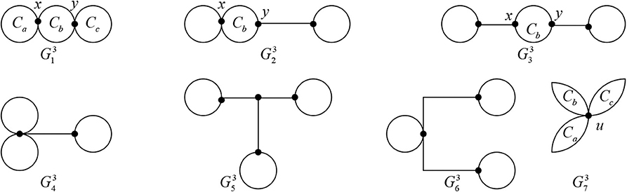
Figure 1. The graphs $G_{i}^{3} (i = 1, 2, \dots, 7)$ .

FIGURE 2

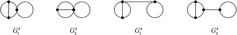
Figure 2. The graphs $G_{i}^{4} (i = 1, 2, \dots, 4)$ .

FIGURE 3

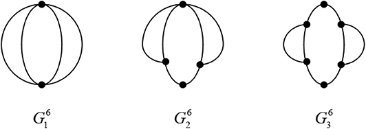
Figure 3. The graphs $G_{i}^{6} (i = 1, 2, 3)$ .

FIGURE 4

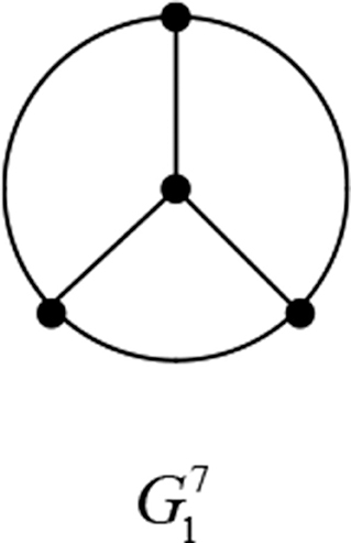
Figure 4. The graph $G_{1}^{7}$ .

Let $T_{1}^{3} (n - 7, 0, 0, 0, 0, 0, 0), T_{1}^{4} (n - 6, 0, 0, 0, 0, 0), T_{1}^{6} (n - 5, 0, 0, 0, 0)$ and $T_{1}^{7} (n - 4, 0, 0, 0)$ be the graphs as shown in Figure 5.

FIGURE 5

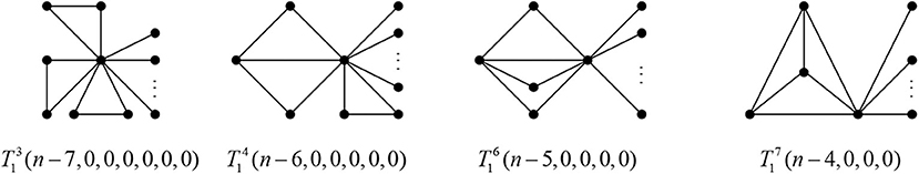
Figure 5. The extremal graphs.

Lemma 2.7. [10]

(i) If $G \in T_{n}^{3}$ , then for every i = 0, 1, …, n, $c_{i} (G) \geq c_{i} (T_{1}^{3} (n - 7, 0, 0, 0, 0, 0, 0))$ , with equality if and only if i ∈ {0, 1, n}.

(ii) If $G \in T_{n}^{4}$ , then for every i = 0, 1, …, n, $c_{i} (G) \geq c_{i} (T_{1}^{4} (n - 6, 0, 0, 0, 0, 0))$ , with equality if and only if i ∈ {0, 1, n}.

(iii) If $G \in T_{n}^{6}$ , then for every i = 0, 1, …, n, $c_{i} (G) \geq c_{i} (T_{1}^{6} (n - 5, 0, 0, 0, 0))$ , with equality if and only if i ∈ {0, 1, n}.

(iv) If $G \in T_{n}^{7}$ , then for every i = 0, 1, …, n, $c_{i} (G) \geq c_{i} (T_{1}^{7} (n - 4, 0, 0, 0))$ , with equality if and only if i ∈ {0, 1, n}.

For i = 3, 4, 6, 7, let $T_{n}^{i, e}$ (resp., $T_{n}^{i, o}$ ) be the set of bipartite tricyclic graphs (resp., non-bipartite tricyclic graphs) in $T_{n}^{i}$ , then $T_{n}^{i} = T_{n}^{i, e} \cup T_{n}^{i, o}$ . From lemmas 2.3 and 2.7, we get

Corollary 2.8. [10]

(i) If $G \in T_{n}^{3, e}$ , then for every i = 0, 1, …, n, $φ_{i} (G) \geq φ_{i} (T_{1}^{3} (n - 7, 0, 0, 0, 0, 0, 0))$ , with equality if and only if i ∈ {0, 1, n}.

(ii) If $G \in T_{n}^{4, e}$ , then for every i = 0, 1, …, n, $φ_{i} (G) \geq φ_{i} (T_{1}^{4} (n - 6, 0, 0, 0, 0, 0))$ , with equality if and only if i ∈ {0, 1, n}.

(iii) If $G \in T_{n}^{6, e}$ , then for every i = 0, 1, …, n, $φ_{i} (G) \geq φ_{i} (T_{1}^{6} (n - 5, 0, 0, 0, 0))$ , with equality if and only if i ∈ {0, 1, n}.

(iv) If $G \in T_{n}^{7, e}$ , then for every i = 0, 1, …, n, $φ_{i} (G) \geq φ_{i} (T_{1}^{7} (n - 4, 0, 0, 0))$ , with equality if and only if i ∈ {0, 1, n}.

Theorem 2.9. [10] Let G be a connected tricyclic graph on n vertices and i be an integer, 0 ≤ i ≤ n. Then $c_{i} (G) \geq c_{i} (T_{1}^{7} (n - 4, 0, 0, 0))$ .

Repeated by lemmas 2.2, 2.5, and 2.6, we get the following conclusion

Theorem 2.10. Let G be a graph in $T_{n}^{3, o} \cup T_{n}^{4, o} \cup T_{n}^{6, o} \cup T_{n}^{7, o}$ . So there is a tricyclic graph G′ with order n, such that G′ ≼ G,. The base of G′ is one of graphs in ${T_{i}^{3} | j = 1, 2, \dots, 9} \cup {T_{i}^{4} | j = 1, 2, \dots, 20} \cup {T_{i}^{6} | j = 1, 2, \dots, 24} \cup {T_{i}^{7} | j = 1, 2, \dots, 7}$ (these base graphs are as shown in Figures 7 –9.

3. The Signless Laplacian Coefficients of Graphs in T_n

Now we consider the minimal element in the partial ordering set ( $T$ _n, ≼).

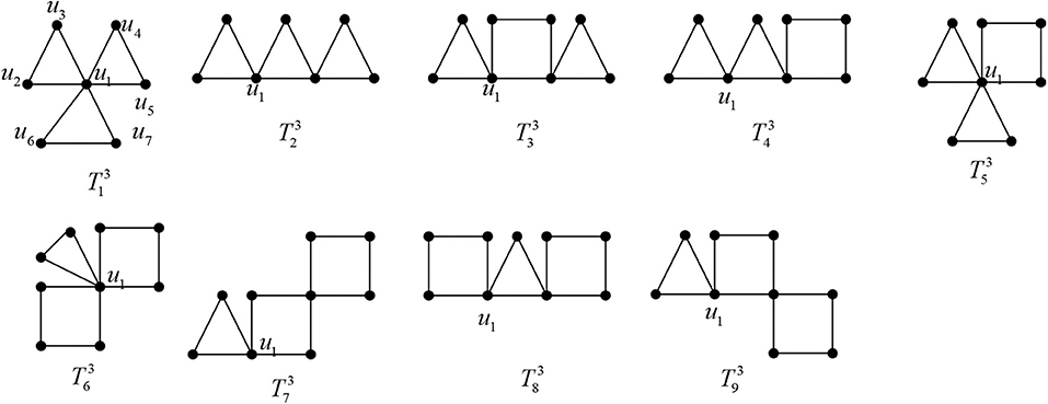
For i = 1, 2, …, 9, let $T_{i}^{3} (s_{1}, s_{2}, \dots, s_{| T_{i}^{3} |})$ be the graph obtained from $T_{i}^{3}$ (as shown in Figure 6) by attaching s_j pendent edges at $u_{j} (j = 1, 2, \dots, | T_{i}^{3} |)$ , where $n = s_{1} + s_{2} + \dots + s_{| T_{i}^{3} |} + | T_{i}^{3} |$ .

FIGURE 6

Figure 6. The graphs $T_{i}^{3} (i = 1, 2, \dots, 9)$ .

Lemma 3.1. For j = 1, 2, …, 9, $T_{j}^{3} (s_{1} + s_{2} + \dots + s_{| T_{j}^{3} |}, 0, \dots, 0) ≼ T_{j}^{3} (s_{1}, s_{2}, \dots, s_{| T_{j}^{3} |})$ , that is, $ϕ_{i} (T_{j}^{3} (s_{1} + s_{2} + \dots + s_{| T_{j}^{3} |}, 0, \dots, 0)) \leq ϕ_{i} (T_{j}^{3} (s_{1}, s_{2}, \dots, s_{| T_{j}^{3} |})), i = 0, 1, \dots, n .$ The equality holds if and only if $s_{2} = \dots = s_{| T_{j}^{3} |} = 0$ .

Proof: For convenience, let $G = T_{j}^{3} (s_{1}, s_{2}, \dots, s_{| T_{j}^{3} |})$ and $G^{'} = T_{j}^{3} (s_{1} + s_{2} + \dots + s_{| T_{j}^{3} |}, 0, \dots, 0)$ for j = 1, 2, …, 9. Note that $ϕ_{0} (G) = 1 = ϕ_{0} (G^{'}), ϕ_{1} (G) = 2 (n + 2) = ϕ_{1} (G^{'})$ . For 2 ≤ i ≤ n, let $H$ and $H$ be the set of all TU-subgraphs of G′ and G with exactly i edges, respectively [3]. Let

\begin{array}{l} H^{^{'} (1)} = {H^{'} \in H | H^{'} c o n t a i n s n o o d d c y c l e}, \\ H^{^{'} (2)} = {H^{'} \in H | H^{'} c o n t a i n s a n o d d c y c l e}, \\ H^{^{'} (3)} = {H^{'} \in H | H^{'} c o n t a i n s t w o o d d c y c l e s} . \end{array}

Similarly for $H$ ⁽¹⁾, $H$ ⁽²⁾, and $H$ ⁽³⁾. We only prove the case for j = 1, the others can be proved similarly.

Let f : $H$ → $H$ with H′ → H = f(H′), where V(H) = V(H′) and

\begin{array}{l} E (H^{'}) = E (H) - {u_{1} x | x \in N_{R^{'}} (u_{1}) \cap N_{G} (u_{2}) \ {u_{3}}} \\ - {u_{1} x | x \in N_{R^{'}} (u_{1}) \cap N_{G} (u_{3}) \ {u_{2}}} \\ - {u_{1} x | x \in N_{R^{'}} (u_{1}) \cap N_{G} (u_{4}) \ {u_{5}}} \\ - {u_{1} x | x \in N_{R^{'}} (u_{1}) \cap N_{G} (u_{5}) \ {u_{4}}} \\ - {u_{1} x | x \in N_{R^{'}} (u_{1}) \cap N_{G} (u_{6}) \ {u_{7}}} \\ - {u_{1} x | x \in N_{R^{'}} (u_{1}) \cap N_{G} (u_{7}) \ {u_{6}}} \\ + {u_{2} x | x \in N_{R^{'}} (u_{1}) \cap N_{G} (u_{2}) \ {u_{3}}} \\ + {u_{3} x | x \in N_{R^{'}} (u_{1}) \cap N_{G} (u_{3}) \ {u_{2}}} \\ + {u_{4} x | x \in N_{R^{'}} (u_{1}) \cap N_{G} (u_{4}) \ {u_{5}}} \\ + {u_{5} x | x \in N_{R^{'}} (u_{1}) \cap N_{G} (u_{5}) \ {u_{4}}} \\ + {u_{6} x | x \in N_{R^{'}} (u_{1}) \cap N_{G} (u_{6}) \ {u_{7}}} \\ + {u_{7} x | x \in N_{R^{'}} (u_{1}) \cap N_{G} (u_{7}) \ {u_{6}}} \end{array}

for R′ being a component of H′ containing u₁. Obviously, f is injective and f( $H$ ′^(k)) ⊆ $H$ ^(k) for j = 1, 2, 3. From the procedure of proof in Theorem 3.1 [10], we have

\begin{array}{l} \sum_{H^{'} \in H^{^{'} (1)}} ω (H^{'}) < \sum_{H \in H^{(1)}} ω (H) . \end{array}

Note that $H$ ′⁽³⁾ = ∅ for j = 1. For H′ ∈ $H$ ′⁽²⁾, without loss of generality, we assume that R′ contains C₃ = u₁u₂u₃u₁ as a subgraph. Let R be the component of H corresponding to R′, obviously, R also contains C₃ = u₁u₂u₃u₁. It is obvious that H′, H have the same number of components and the product of the order of components which contain no u_i(i = 1, 2, …, 7) of H′ is the same as H. The order of the tree components of H′, which include at least one of u_i(i = 4, …, 7) are no more than the corresponding ones of H, then ω(f(H′)) ≥ ω(H′). Hence

\begin{array}{l} ϕ_{i} (G) = \sum_{H \in H^{(1)}} ω (H) + \sum_{H \in H^{(2)}} ω (H) + \sum_{H \in H^{(3)}} ω (H) \\ \geq \sum_{H^{'} \in H^{^{'} (1)}} ω (H^{'}) + \sum_{H^{'} \in H^{^{'} (2)}} ω (H^{'}) + \sum_{H^{'} \in H^{^{'} (3)}} ω (H^{'}) = ϕ_{i} (G^{'}) . \end{array}

The equality holds if and only if s₂ = ⋯ = s₇ = 0.□

For i = 1, 2, …, 20, let $T_{i}^{4} (s_{1}, s_{2}, \dots, s_{| T_{i}^{4} |})$ be the graph obtained from $T_{i}^{4}$ (as shown in Figure 7) by attaching s_j pendent edges at $u_{j} (j = 1, 2, \dots, | T_{i}^{4} |)$ , where $n = s_{1} + s_{2} + \dots + s_{| T_{i}^{4} |} + | T_{i}^{4} |$ . Similar to the proof of Lemma 3.1, we have

FIGURE 7

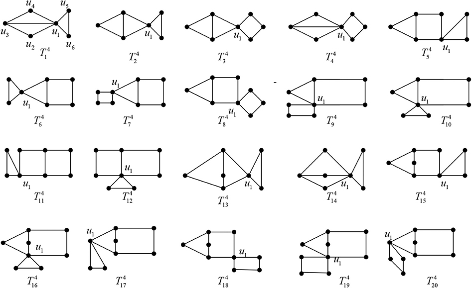
Figure 7. The graphs $T_{i}^{4} (i = 1, 2, \dots, 20)$ .

Lemma 3.2. For j = 1, 2, …, 20, $T_{j}^{4} (s_{1} + s_{2} + \dots + s_{| T_{j}^{4} |}, 0, \dots, 0) ≼ T_{j}^{4} (s_{1}, s_{2}, \dots, s_{| T_{j}^{4} |})$ , that is, $ϕ_{i} (T_{j}^{4} (s_{1} + s_{2} + \dots + s_{| T_{j}^{4} |}, 0, \dots, 0)) \leq ϕ_{i} (T_{j}^{4} (s_{1}, s_{2}, \dots, s_{| T_{j}^{4} |})), i = 0, 1, \dots, n .$ The equality holds if and only if $s_{2} = \dots = s_{| T_{j}^{4} |} = 0$ .

For i = 1, 2, …, 7, let $T_{i}^{7} (s_{1}, s_{2}, \dots, s_{| T_{i}^{7} |})$ be the graph obtained from $T_{i}^{7}$ (as shown in Figure 8) by attaching s_j pendent edges at $u_{j} (j = 1, 2, \dots, | T_{i}^{7} |)$ , where $n = s_{1} + s_{2} + \dots + s_{| T_{i}^{7} |} + | T_{i}^{7} |$ . Similar to the proof of Lemma 3.1, we have

FIGURE 8

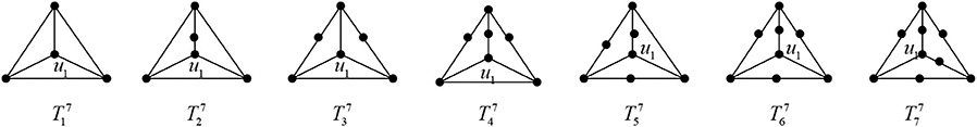
Figure 8. The graphs $T_{i}^{7} (i = 1, 2, \dots, 7)$ .

Lemma 3.3. For j = 1, 2, …, 7, $T_{j}^{7} (s_{1} + s_{2} + \dots + s_{| T_{j}^{7} |}, 0, \dots, 0) ≼ T_{j}^{7} (s_{1}, s_{2}, \dots, s_{| T_{j}^{7} |})$ , that is, $ϕ_{i} (T_{j}^{7} (s_{1} + s_{2} + \dots + s_{| T_{j}^{7} |}, 0, \dots, 0)) \leq ϕ_{i} (T_{j}^{7} (s_{1}, s_{2}, \dots, s_{| T_{j}^{7} |})), i = 0, 1, \dots, n .$ The equality holds if and only if $s_{2} = \dots = s_{| T_{j}^{7} |} = 0$ .

For i = 1, 2, …, 24, let $T_{i}^{6} (s_{1}, s_{2}, \dots, s_{| T_{i}^{6} |})$ be the graph obtained from $T_{i}^{6}$ (as shown in Figure 9) by attaching s_j pendent edges at $u_{j} (j = 1, 2, \dots, | T_{i}^{6} |)$ , where $n = s_{1} + s_{2} + \dots + s_{| T_{i}^{6} |} + | T_{i}^{6} |$ . Similar to the proof of Lemma 3.1, we have

FIGURE 9

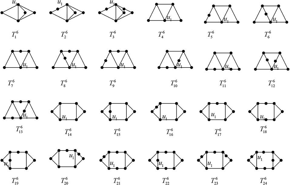
Figure 9. The graphs $T_{i}^{6} (i = 1, 2, \dots, 24)$ .

Lemma 3.4. For j = 1, 2, …, 24, $T_{j}^{6} (s_{1} + s_{2} + \dots + s_{| T_{j}^{6} |}, 0, \dots, 0) ≼ T_{j}^{6} (s_{1}, s_{2}, \dots, s_{| T_{j}^{6} |})$ , that is, $ϕ_{i} (T_{j}^{6} (s_{1} + s_{2} + \dots + s_{| T_{j}^{6} |}, 0, \dots, 0)) \leq ϕ_{i} (T_{j}^{6} (s_{1}, s_{2}, \dots, s_{| T_{j}^{6} |})), i = 0, 1, \dots, n .$ The equality holds if and only if $s_{2} = \dots = s_{| T_{j}^{6} |} = 0$ .

Lemma 3.5. For $n \geq | T_{j}^{3} | (j = 1, 2, \dots, 9)$ ,

(i) $T_{2}^{3} (n - 7, 0, 0, 0, 0, 0, 0) ≽ T_{1}^{3} (n - 7, 0, 0, 0, 0, 0, 0)$ .

(ii) $T_{j}^{3} (n - 8, 0, 0, 0, 0, 0, 0, 0) ≽ T_{5}^{3} (n - 8, 0, 0, 0, 0, 0, 0, 0, 0)$ for j = 3, 4.

(iii) $T_{j}^{3} (n - 9, 0, 0, 0, 0, 0, 0, 0, 0) ≽ T_{6}^{3} (n - 9, 0, 0, 0, 0, 0, 0, 0, 0)$ for j = 7, 8, 9.

Proof: (i) We have

\begin{array}{l} Q (T_{2}^{3} (n - 7, 0, \dots, 0)) - Q (T_{1}^{3} (n - 7, 0, 0, 0, 0, 0, 0)) \\ = {(x - 1)}^{n - 8} [2 (n - 5) x^{6} - (18 n - 90) x^{5} + (62 n - 302) x^{4} \\ - (102 n - 462) x^{3} \\ + (80 n - 296) x^{2} - (24 n - 24) x + 32] . \end{array}

Further by Lemma 2.3, $T_{2}^{3} (n - 7, 0, 0, 0, 0, 0, 0) ≽ T_{1}^{3} (n - 7, 0, 0, 0, 0, 0, 0)$ .

\begin{array}{l} Q (T_{3}^{3} (n - 8, 0, 0, 0, 0, 0, 0, 0, 0)) - Q (T_{5}^{3} (n - 8, 0, 0, 0, 0, 0, 0, 0, 0)) \\ = {(x - 1)}^{n - 9} [(2 n - 12) x^{7} - (22 n - 132) x^{6} + (96 n - 568) x^{5} \\ - (212 n - 1208) x^{4} \\ + (250 n - 1308) x^{3} - (150 n - 628) x^{2} + (36 n - 32) x - 48], \\ Q (T_{4}^{3} (n - 8, 0, 0, 0, 0, 0, 0, 0, 0)) - Q (T_{5}^{3} (n - 8, 0, 0, 0, 0, 0, 0, 0, 0)) \\ = {(x - 1)}^{n - 9} [(2 n - 11) x^{7} - (23 n - 125) x^{6} + (104 n - 546) x^{5} \\ - (233 n - 1128) x^{4} \\ + (266 n - 1047) x^{3} - (140 n - 219) x^{2} + (24 n + 200) x - 68], \\ Q (T_{7}^{3} (n - 9, 0, 0, 0, 0, 0, 0, 0, 0)) - Q (T_{6}^{3} (n - 9, 0, 0, 0, 0, 0, 0, 0, 0)) \\ = {(x - 1)}^{n - 10} [(2 n - 14) x^{8} - (26 n - 182) x^{7} + (138 n - 958) x^{6} \\ - (382 n - 2594) x^{5} \\ + (580 n - 3748) x^{4} - (456 n - 5608) x^{3} + (144 n - 464) x^{2} - 192 x], \\ Q (T_{8}^{3} (n - 9, 0, 0, 0, 0, 0, 0, 0, 0)) - Q (T_{6}^{3} (n - 9, 0, 0, 0, 0, 0, 0, 0, 0)) \\ = {(x - 1)}^{n - 10} [(2 n - 14) x^{8} - (26 n - 182) x^{7} + (138 n - 948) x^{6} \\ - (364 n - 2512) x^{5} \\ + (520 n - 3520) x^{4} - (368 n - 2400) x^{3} + (96 n - 576) x^{2}], \\ Q (T_{9}^{3} (n - 9, 0, 0, 0, 0, 0, 0, 0, 0)) - Q (T_{6}^{3} (n - 9, 0, 0, 0, 0, 0, 0, 0, 0)) \\ = {(x - 1)}^{n - 10} [(2 n - 14) x^{8} - (26 n - 182) x^{7} + (136 n - 944) x^{6} \\ - (364 n - 2468) x^{5} \\ + (522 n - 3350) x^{4} - (378 n - 2102) x^{3} + (108 n - 300) x^{2} - 144 x] . \end{array}

So (ii) and (iii) hold.□

Lemma 3.6. For $n \geq | T_{j}^{4} | (j = 1, \dots, 20)$ ,

(i) $T_{j}^{4} (n - | T_{j}^{4} |, 0, \dots, 0) ≽ T_{1}^{4} (n - 6, 0, \dots, 0)$ for j = 2, 5, 6, 10, 15, 16, 17

(ii) $T_{j}^{4} (n - | T_{j}^{4} |, 0, \dots, 0) ≽ T_{4}^{4} (n - 7, 0, \dots, 0)$ for j = 3, 7, 8, 9, 18, 19, 20.

(iii) $T_{j}^{4} (n - | T_{j}^{4} |, 0, \dots, 0) ≽ T_{14}^{4} (n - 7, 0, \dots, 0)$ for j = 11, 12, 13.

Proof:

\begin{array}{l} Q (T_{2}^{4} (n - 6, 0, \dots, 0)) - Q (T_{1}^{4} (n - 6, 0, \dots, 0)) \\ = {(x - 1)}^{n - 7} [(n - 4) x^{5} - (8 n - 32) x^{4} + (23 n - 88) x^{3} \\ - (28 n - 92) x^{2} + (12 n - 16) x - 16], \\ Q (T_{3}^{4} (n - 7, 0, \dots, 0)) - Q (T_{4}^{4} (n - 7, 0, \dots, 0)) \\ = {(x - 1)}^{n - 8} [(n - 5) x^{6} - (10 n - 50) x^{5} + (38 n - 188) x^{4} \\ - (68 n - 382) x^{3} + \\ (56 n - 256) x^{2} - (16 n - 64) x], \\ Q (T_{11}^{4} (n - 8, 0, \dots, 0)) - Q (T_{14}^{4} (n - 7, 0, \dots, 0)) \\ = {(x - 1)}^{n - 9} [(2 n - 10) x^{7} - (24 n - 120) x^{6} + (110 n - 539) x^{5} \\ - (241 n - 1107) x^{4} + \\ (255 n - 971) x^{3} - (111 n - 161) x^{2} + (9 n + 144) x - 12], \end{array}

By the results of Appendix, the results hold.

Lemma 3.7. For $n \geq | T_{j}^{7} | (j = 1, \dots, 7)$ , $T_{j}^{7} (n - | T_{j}^{7} |, 0, \dots, 0) ≽ T_{1}^{7} (n - 4, 0, 0, 0)$ .

Proof: We have

\begin{array}{l} Q (T_{2}^{7} (n - 5, 0, \dots, 0)) - Q (T_{1}^{7} (n - 4, 0, \dots, 0)) \\ = {(x - 1)}^{n - 6} [(n - 3) x^{4} - (8 n - 28) x^{3} + (18 n - 68) x^{2} \\ - (12 n - 48) x], \\ Q (T_{3}^{7} (n - 6, 0, \dots, 0)) - Q (T_{1}^{7} (n - 4, 0, \dots, 0)) \\ = {(x - 1)}^{n - 7} [(2 n - 7) x^{5} - (19 n - 73) x^{4} + (55 n - 213) x^{3} \\ - (57 n - 199) x^{2} + (19 n - 40) x - 12], \\ Q (T_{4}^{7} (n - 7, 0, \dots, 0)) - Q (T_{1}^{7} (n - 4, 0, \dots, 0)) \\ = {(x - 1)}^{n - 8} [(3 n - 12) x^{6} - (33 n - 140) x^{5} + (126 n - 536) x^{4} \\ - (210 n - 828) x^{3} + (151 n - 432) x^{2} - (37 n + 48) x + 60], \\ Q (T_{5}^{7} (n - 7, 0, \dots, 0)) - Q (T_{1}^{7} (n - 4, 0, \dots, 0)) \\ = {(x - 1)}^{n - 8} [(3 n - 12) x^{6} - (33 n - 140) x^{5} + (126 n - 540) x^{4} \\ - (210 n - 858) x^{3} + (152 n - 514) x^{2} - (39 n + 36) x + 39], \\ Q (T_{6}^{7} (n - 8, 0, \dots, 0)) - Q (T_{1}^{7} (n - 4, 0, \dots, 0)) \\ = {(x - 1)}^{n - 9} [(4 n - 18) x^{7} - (50 n - 238) x^{6} + (233 n - 1139) x^{5} \\ - (521 n - 2541) x^{4} + (584 n - 2713) x^{3} \\ - (301 n - 1171) x^{2} + (50 n - 40) - 32], \\ Q (T_{7}^{7} (n - 9, 0, \dots, 0)) - Q (T_{1}^{7} (n - 4, 0, \dots, 0)) \\ = {(x - 1)}^{n - 10} [(5 n - 25) x^{8} ​ - ​ (70 n - 368) x^{7} + ​ (385 n - 2086) x^{6} \\ - (1085 n - 5938) x^{5} ​ + (2684 n - ​ 9039) x^{4} ​ - (1415 n - 7004) x^{3} \\ + (572 n - 21122) x^{2} - (76 n + 128) x + 80] . \end{array}

So the results hold.□

Theorem 3.8. For $G \in T_{n}^{3} \cup T_{n}^{4} \cup T_{n}^{7}$ , $G ≽ T_{1}^{7} (n - 4, 0, 0, 0)$ . The equality holds if and only if $G ≅ T_{1}^{7} (n - 4, 0, 0, 0) .$

Proof: If $G \in T_{n}^{3, e} \cup T_{n}^{4, e} \cup T_{n}^{7, e}$ , by Theorem 2.9, the results hold.

If $G \in T_{n}^{3, o} \cup T_{n}^{4, o} \cup T_{n}^{7, o}$ , by direct calculation, we have

\begin{array}{l} Q (T_{1}^{3} (n - 7, 0, \dots, 0)) - Q (T_{1}^{7} (n - 4, 0, \dots, 0)) \\ = {(x - 1)}^{n - 8} [3 x^{6} - (3 n + 16) x^{5} + (16 n + 54) x^{4} \\ - (30 n + 156) x^{3} + (24 n + 259) x^{2} - (7 n + 204) x + 60] \\ Q (T_{5}^{3} (n - 8, 0, \dots, 0)) - Q (T_{1}^{7} (n - 4, 0, \dots, 0)) \\ = {(x - 1)}^{n - 9} [n x^{7} - (14 n - 16) x^{6} + (66 n - 84) x^{5} \\ - (144 n - 108) x^{4} + (157 n + 100) x^{3} - (82 n + 316) x^{2} \\ + (16 n + 224) x - 48], \\ Q (T_{6}^{3} (n - 9, 0, \dots, 0)) - Q (T_{1}^{7} (n - 4, 0, \dots, 0)) \\ = {(x - 1)}^{n - 10} [(2 n - 4) x^{8} - (28 n - 70) x^{7} + (148 n - 391) x^{6} \\ - (393 n - 994) x^{5} + (570 n - 1221) x^{4} \\ - (451 n - 616) x^{3} + (180 n + 16) x^{2} - (28 n + 96) x + 16], \\ Q (T_{1}^{4} (n - 6, 0, \dots, 0)) - Q (T_{1}^{7} (n - 4, 0, \dots, 0)) \\ = {(x - 1)}^{n - 7} [2 x^{5} - (2 n + 8) x^{4} + (8 n + 26) x^{3} \\ - (10 n + 68) x^{2} + (4 n + 80) x - 32] \\ Q (T_{4}^{4} (n - 7, 0, \dots, 0)) - Q (T_{1}^{7} (n - 4, 0, \dots, 0)) \\ = {(x - 1)}^{n - 8} [(n - 1) x^{6} - (12 n - 22) x^{5} + (46 n - 85) x^{4} \\ - (75 n - 96) x^{3} + (52 n + 16) x^{2} - (12 n + 64) x + 16] \\ Q (T_{14}^{4} (n - 7, 0, \dots, 0)) - Q (T_{1}^{7} (n - 4, 0, \dots, 0)) \\ = {(x - 1)}^{n - 8} [(n - 1) x^{6} - (12 n - 24) x^{5} + (47 n - 107) x^{4} \\ - (80 n - 176) x^{3} + (60 n - 108) x^{2} - (16 n - 16) x] . \end{array}

Further by Theorem 2.10 and lemmas 3.2–3.4, 3.6–3.8, we have $G ≽ T_{1}^{7} (n - 4, 0, 0, 0)$ .□

Lemma 3.9. For $n \geq | T_{j}^{6} | (j = 1, \dots, 9, 11, \dots, 24)$ , $T_{j}^{6} (n - | T_{j}^{6} |, 0, \dots, 0) ≽ T_{1}^{6} (n - 4, 0, 0, 0)$ .

Proof: We have

\begin{array}{l} Q (T_{2}^{6} (n - 6, 0, \dots, 0)) - Q (T_{1}^{6} (n - 5, 0, \dots, 0)) \\ = {(x - 1)}^{n - 7} [(n - 3) x^{5} - (9 n - 29) x^{4} + (25 n - 76) x^{3} \\ - (26 n - 56) x^{2} + (8 n + 16) x - 16] \end{array}

By the results of Appendix, the results hold.□

Theorem 3.10. For $G \in T_{n}^{6}$ , $G ≽ T_{10}^{6} (n - 5, 0, 0, 0)$ or $G ≽ T_{1}^{6} (n - 5, 0, 0, 0)$ . The equality holds if and only if $G ≅ T_{1}^{6} (n - 5, 0, 0, 0, 0)$ or $G ≅ T_{10}^{6} (n - 5, 0, 0, 0) .$

Proof: If $G \in T_{n}^{6, e}$ , by Theorem 2.9 and

\begin{array}{l} Q (T_{1}^{6} (n - 5, 0, \dots, 0)) - Q (T_{1}^{7} (n - 4, 0, \dots, 0)) = 0 & (1) \end{array}

we have $G ≽ T_{1}^{6} (n - 5, 0, 0, 0)$ .

If $G \in T_{n}^{6, o}$ , by Theorem 2.10, lemmas 3.5 and 3.9, we have $G ≽ T_{10}^{6} (n - 7, 0, \dots, 0)$ or $G ≽ T_{1}^{6} (n - 5, 0, 0, 0)$ .□

Remark: By (3.1), $T_{1}^{6} (n - 5, 0, \dots, 0)$ and $T_{1}^{7} (n - 4, 0, \dots, 0)$ have the same signless Laplacian characteristic polynomials.

Theorem 3.11. $T_{10}^{6} (n - 7, 0, \dots, 0), T_{1}^{6} (n - 5, 0, 0, 0), T_{1}^{7} (n - 4, 0, 0, 0)$ are the only three minimal elements in the partial set ( $T$ _n, ≽).

Proof: By (3.1), theorems 3.8 and 3.10, it is obvious that $T_{1}^{6} (n - 5, 0, 0, 0), T_{1}^{7} (n - 4, 0, 0, 0)$ are the minimal elements in the partial set ( $T$ _n, ≽).

Note that if there is a graph G₀ in $T_{n}^{3} \cup T_{n}^{4} \cup T_{n}^{6, e} \cup T_{n}^{7}$ such that $T_{10}^{6} (n - 7, 0, \dots, 0) ≽ G_{0}$ , then by Theorem 3.8 and (3.1), we have $T_{10}^{6} (n - 7, 0, \dots, 0) ≽ T_{1}^{6} (n - 5, 0, 0, 0) .$ But

\begin{array}{l} Q (T_{10}^{6} (n - 7, 0, \dots, 0)) - Q (T_{1}^{6} (n - 5, 0, \dots, 0)) \\ = {(x - 1)}^{n - 8} [(2 n - 6) x^{6} - (22 n - 76) x^{5} + (83 n - 308) x^{4} \\ - (137 n - 542) x^{3} \\ + (98 n - 448) x^{2} - (24 n - 192) x - 48], \end{array}

it is a contradiction.

Hence the results hold.□

4. The Incidence Energy of Tricyclic Graphs

The incidence energy IE(G) of a graph G is defined to be the sum of the square root of all eigenvalues of Q(G)[3].

Theorem 4.1. [11] Let G and G′ be two graphs of order n, if $φ_{k} (G) ≼ φ_{k} (G^{'})$ for 1 ≤ k ≤ n, then IE(G) ≤ IE(G′). In particular, if at least one of inequalities is strict, then IE(G) < IE(G′).

Theorem 4.2. If G ∈ $T$ _n, then $I E (G) \geq I E (T_{1}^{6} (n - 5, 0, 0, 0, 0)) = I E (T_{1}^{7} (n - 4, 0, 0, 0)) .$ The equality holds if and only if $G ≅ T_{1}^{6} (n - 5, 0, 0, 0, 0),$ or $G ≅ T_{1}^{7} (n - 4, 0, 0, 0) .$

Proof: By Theorem 3.11, we have

$I E (G) \geq m i n {I E (T_{10}^{6} (n - 7, 0, \dots, 0)), I E (T_{1}^{6} (n - 5, 0, 0, 0, 0)), I E (T_{1}^{7} (n - 4, 0, 0, 0))} .$ Note that

\begin{array}{l} Q (T_{1}^{7} (n - 4, 0, \dots, 0)) = {(x - 1)}^{n - 5} [(x^{5} - (n + 9) x^{4} \\ + (9 n + 24) x^{3} - (24 n + 32) x^{2} \\ + (20 n + 48) x - 48] \\ = {(x - 1)}^{n - 5} {(x - 2)}^{2} [x^{3} - (n + 5) x^{2} \\ + 5 n x - 12], \\ Q (T_{10}^{6} (n - 7, 0, \dots, 0)) = x {(x - 1)}^{n - 8} [(x^{7} - (n + 12) x^{6} \\ + (14 n + 48) x^{5} - (76 n + 56) x^{4} + \\ (203 n - 83) x^{3} - (278 n - 230) x^{2} \\ + (182 n - 128) x - 44 n] \\ = x {(x - 1)}^{n - 7} (x - 2) [x^{5} - (n + 9) x^{4} \\ + (11 n + 19) x^{3} - (41 n - 19) x^{2} \\ + (58 n - 64) x - 22 n] . \end{array}

Let α₁ ≥ α₂ ≥ α₃ be the roots of x³ − (n + 5)x² + 5nx − 12 = 0, and β₁ ≥ β₂ ≥ β₃ ≥ β₄ ≥ β₅ be the roots of x⁵ − (n + 9)x⁴ + (11n + 19)x³ − (41n − 19)x² + (58n − 64)x − 22n = 0, then

\begin{array}{l} I E (T_{1}^{7}) = (n - 5) + 2 \sqrt{2} + \sqrt{α_{1}} + \sqrt{α_{2}} + \sqrt{α_{3}} \\ I E (T_{10}^{6}) = (n - 7) + \sqrt{2} + \sqrt{β_{1}} + \sqrt{β_{2}} + \sqrt{β_{3}} + \sqrt{β_{4}} + \sqrt{β_{5}} . \end{array}

If n ≤ 40, by Matlab7.0 it is easy to see $I E (T_{10}^{6}) > I E (T_{1}^{7})$ holds.

If n ≥ 40, it is easy to see that n − 0.07 ≤ α₁ ≤ n + 0.07, 4.93 ≤ α₂ ≤ 5, 0 ≤ α₃ ≤ 0.07 and n − 1.98 ≤ β₁ ≤ n − 1.9, 4.58 ≤ β₂ ≤ 4.62, 3.41 ≤ β₃ ≤ 3.42, 2.37 ≤ β₄ ≤ 2.39, 0.54 ≤ β₅ ≤ 0.55.

\begin{array}{l} 6.261 + \sqrt{n - 1.98} \leq \sum_{i = 1}^{5} \sqrt{β_{i}} \leq 6.286 + \sqrt{n - 1.9}, \\ 2.22 + \sqrt{n - 0.07} \leq \sum_{i = 1}^{3} \sqrt{α_{i}} \leq 2.5 + \sqrt{n + 0.07}, \\ 3.597 \leq \sum_{i = 1}^{5} \sqrt{β_{i}} - \sum_{i = 1}^{3} \sqrt{α_{i}} \leq 3.92 . \end{array}

It is easy to see that

\begin{array}{l} I E (T_{10}^{6}) - I E (T_{1}^{7}) = \sum_{i = 1}^{5} \sqrt{β_{i}} - \sum_{i = 1}^{3} \sqrt{α_{i}} - 2 - \sqrt{2} \\ \geq 3.597 - 2 - \sqrt{2} > 0 . \end{array}

So the assertions hold.□

5. Conclusion and Extension

This paper propose an appropriate graph transformation to reflect the monotonicity of the coefficients, and give a sharp lower bound for incidence energy in the class of tricyclic graphs and characterize the extremal structures. The study on boundary of the incidence energy and its extremum structure of tricyclic graphs enriches and develops the study of the graph structure, but also connects the mathematical branch with other disciplines such as biology, physics and chemistry. It promotes the development of some theories of graph theory. It promotes the development of graph structure, the development of graph theory, and the study of graph theory and its application. For example, mathematical biology, application of graph theory in power system, molecular structure based on graph theory. Furthermore, similar to the graph energy, the incidence energy also reflects some physical and chemical properties of conjugated molecules, such as melting point and boiling point, this provides a theoretical reference for the researchers of the synthesis of new materials and new materials, and saves the cost for the development of new materials and new materials to a certain extent. Based on the extensive application of graph theory in many fields, the findings of this study have many important implications for future practice.

Data Availability Statement

The original contributions presented in the study are included in the article/Supplementary Materials, further inquiries can be directed to the corresponding author/s.

Author Contributions

ZZ contributed to the conception of the study, performed the data analyses, and wrote the manuscript. HL contributed significantly to analysis and manuscript preparation and helped to perform the analysis with constructive discussions.

Funding

This work was supported by the Scientific Research Project of Education Department of Shaanxi Province (19JK0906).

Conflict of Interest

The authors declare that the research was conducted in the absence of any commercial or financial relationships that could be construed as a potential conflict of interest.

Supplementary Material

The Supplementary Material for this article can be found online at: https://www.frontiersin.org/articles/10.3389/fphy.2020.00208/full#supplementary-material

References

1. Bollobás B. Modern Graph Theory. Berlin; New York, NY: Springer-Verlag (1998). doi: 10.1007/978-1-4612-0619-4

CrossRef Full Text | Google Scholar

2. Cvetković D, Simić S. Towards a spectral theory of graphs based on the signless Laplacian. Int Publ Inst Math. (2009) 85:19–33. doi: 10.1016/j.laa.2009.05.020

CrossRef Full Text

3. Zhang J, Zhang X. The signless Laplacian coefficients and incidence energy of bicyclic graphs. Linear Algebra Appl. (2013) 439:385–6. doi: 10.1016/j.laa.2013.10.026

CrossRef Full Text | Google Scholar

4. Lin HQ, Hong Y, Shu JL. Some relations between the eigenvalues of adjacency, Laplacian and signless Laplacian mattrix of a graph. Graphs Combin. (2015) 31:669–71. doi: 10.1007/s00373-013-13980-5

CrossRef Full Text | Google Scholar

5. Mohar B. On the Laplacian coefficients of acyclic graphs. Linear Algebra Appl. (2007) 722:736–41. doi: 10.1016/j.laa.2006.12.005

CrossRef Full Text | Google Scholar

6. Stevanović D, Ilić A. On the Laplacian coefficients of unicyclic graphs. Linear Algebra Appl. (2009) 430:2290–300. doi: 10.1016/j.laa.2008.12.006

CrossRef Full Text | Google Scholar

7. Li HH, Tam BS, Su L. On the signless Laplcaian coefficients of unicyclic graphs. Linear Algebra Appl. (2013) 439:2008–28. doi: 10.1016/j.laa.2013.05.030

CrossRef Full Text | Google Scholar

8. He CX, Shan HY. On the Laplacian coefficients of bicyclic graphs. Discrete Math. (2010) 310:3404–12. doi: 10.1016/j.disc.2010.08.012

CrossRef Full Text | Google Scholar

9. Zhu ZX, Lu HY. On the general sun-connectivity index of tricyclic graphs. J Appl Math Comput. (2016) 51:177–88. doi: 10.1007/s12190-015-0898-2

CrossRef Full Text | Google Scholar

10. Pai X, Liu S, Guo J. On the Laplacian coefficients of tricyclic graphs. J Math Anal Appl. (2013) 405:200–8. doi: 10.1016/j.jmaa.2013.03.059

CrossRef Full Text | Google Scholar

11. Mirzakhah M, Kiani D. Some results on signless Laplacian coefficients of graphs. Linear Algebra Appl. (2012) 437:2243–51. doi: 10.1016/j.laa.2012.05.022

CrossRef Full Text | Google Scholar

12. Liu JB, Zhao J, Cai Z. On the generalized adjacency, Laplacian and signless Laplacian spectra of the weighted edge corona networks. Phys A. (2020) 540:123073. doi: 10.1016/j.physa.2019.123073

CrossRef Full Text | Google Scholar

13. Merris R. Laplacian matrices of graphs. Linear Algebra Appl. (1994) 197–8:143–76. doi: 10.1016/0024-3795(94)90486-3

CrossRef Full Text | Google Scholar

14. Cvetković D, Rowlinson P, Simić S. Singless Laplacians of finite graphs. Linear Algebra Appl. (2007) 432:155–71. doi: 10.1109/ICACIA.2010.5709937

CrossRef Full Text | Google Scholar

15. Tan SW. On the Laplacian coefficients of unicyclic graphs with prescribed matching number. Discrete Math. (2011) 311:582–94. doi: 10.1016/j.disc.2010.12.022

CrossRef Full Text | Google Scholar

16. Hoffman AJ, Smith JH. On the spectral radii of topologically equivalent graphs. In: Fiedler, Editor. Recent Advances in Graph Theory. New York, NY: Academia Praha (1975). p. 273–81.

17. Guo S. On the spectral radius of bicycle graphs with n vertics and diameter d. Linear Algebra Appl. (2007) 422:119–32. doi: 10.1016/j.laa.2006.09.011

CrossRef Full Text | Google Scholar

18. Tan SW. On the Laplacian coefficients and Laplacian-like energy of bicyclic graphs. Linear Multilin AlgebRA. (2012) 60:1071–92. doi: 10.1080/03081087.2011.643473

CrossRef Full Text | Google Scholar

19. Wang WH, Zhong L, Zheng LJ. The signless Laplacian coefficients and the incidence energy of the graphs without even cycles. Linear Algebra Appl. (2019) 563:476–93. doi: 10.1016/j.laa.2018.10.025

CrossRef Full Text | Google Scholar

20. Li SC, Li XC, Zhu ZX. On tricyclic graphs with minimal energy. Match-Commun Math Comput Chem. (2008) 59:397–419. doi: 10.1111/j.1467-9892.2007.00552.x

CrossRef Full Text | Google Scholar

Keywords: incidence energy, extremal graph, tricyclic graph, Laplacian matrix, signless Laplacian coefficients

Citation: Lu H and Zhu Z (2020) On the Boundary of Incidence Energy and Its Extremum Structure of Tricycle Graphs. Front. Phys. 8:208. doi: 10.3389/fphy.2020.00208

Received: 20 March 2020; Accepted: 15 May 2020;
Published: 19 June 2020.

Edited by:

Muhammad Javaid, University of Management and Technology, Pakistan

Reviewed by:

Sunil Kumar, National Institute of Technology, Jamshedpur, India
Boyi He, Sichuan Normal University, China
Zixuan Yang, Xi'an Jiaotong University, China

Copyright © 2020 Lu and Zhu. This is an open-access article distributed under the terms of the Creative Commons Attribution License (CC BY). The use, distribution or reproduction in other forums is permitted, provided the original author(s) and the copyright owner(s) are credited and that the original publication in this journal is cited, in accordance with accepted academic practice. No use, distribution or reproduction is permitted which does not comply with these terms.

*Correspondence: Hongyan Lu, lhyy116@163.com; Zhongxun Zhu, zzxun73@163.com

BRIEF RESEARCH REPORT article

On the Boundary of Incidence Energy and Its Extremum Structure of Tricycle Graphs

1. Introduction

2. Preliminaries

3. The Signless Laplacian Coefficients of Graphs in T_n

4. The Incidence Energy of Tricyclic Graphs

5. Conclusion and Extension

Data Availability Statement

Author Contributions

Funding

Conflict of Interest

Supplementary Material

References

This article is part of the Research Topic

People also looked at

BRIEF RESEARCH REPORT article

On the Boundary of Incidence Energy and Its Extremum Structure of Tricycle Graphs

1. Introduction

2. Preliminaries

3. The Signless Laplacian Coefficients of Graphs in Tn

4. The Incidence Energy of Tricyclic Graphs

5. Conclusion and Extension

Data Availability Statement

Author Contributions

Funding

Conflict of Interest

Supplementary Material

References

This article is part of the Research Topic

People also looked at

3. The Signless Laplacian Coefficients of Graphs in T_n