Classifying Wood Properties of Loblolly Pine Grown in Southern Brazil Using NIR-Hyperspectral Imaging
by
 , ,
, ,
Laurence Schimleck
1,*, 
Jorge L. M. Matos
2 ,
,
Antonio Higa
2,
Rosilani Trianoski
2,
José G. Prata
2 and
Joseph Dahlen
3 1
Department of Wood Science and Engineering, College of Forestry, Oregon State University, Corvallis, OR 97331, USA
2
Department of Wood Science and Technology, Federal University of Paraná, 80.210-170 Curitiba, Brazil
3
Warnell School of Forestry and Natural Resources, University of Georgia, Athens, GA 30602, USA
*
Author to whom correspondence should be addressed.
Forests 2020, 11(6), 686; https://doi.org/10.3390/f11060686
Submission received: 29 May 2020
/
Revised: 10 June 2020
/
Accepted: 16 June 2020
/
Published: 18 June 2020
(This article belongs to the Section Wood Science and Forest Products)
Abstract
:Loblolly pine (Pinus taeda L.) is one of the most important commercial timber species in the world. While the species is native to the southeastern United States of America (USA), it has been widely planted in southern Brazil, where it is the most commonly planted exotic species. Interest exists in utilizing nondestructive testing methods for wood property assessment to aid in improving the wood quality of Brazilian grown loblolly pine. We used near-infrared hyperspectral imaging (NIR-HSI) on increment cores to provide data representative of the radial variation of families sampled from a 10-year-old progeny test located in Rio Negrinho municipality, Santa Catarina, Brazil. Hyperspectral images were averaged to provide an individual NIR spectrum per tree for cluster analysis (hierarchical complete linkage with square Euclidean distance) to identify trees with similar wood properties. Four clusters (0, 1, 2, 3) were identified, and based on SilviScan data for air-dry density, microfibril angle (MFA), and stiffness, clusters differed in average wood properties. Average ring data demonstrated that trees in Cluster 0 had the highest average ring densities, and those in Cluster 3 the lowest. Cluster 3 trees also had the lowest ring MFAs. NIR-HSI provides a rapid approach for collecting wood property data and, when coupled with cluster analysis, potentially, allows screening for desirable wood properties amongst families in tree improvement programs.
1. Introduction
Increasingly, plantation forests are being relied upon to supply society with a multitude of fiber products. The shift from harvesting native forests to plantations has occurred in many countries, and subsequently, there has been a substantial increase in the total area of plantations globally (estimated to be 278 million ha in 2015, up from 167.5 million ha in 1990) [1]. At 7.83 million ha, Brazil has one of the largest plantation estates in the world and also one of the highest utilization rates (91%) of plantation-grown wood for industrial needs. A number of exotic species are planted in Brazil, with pines representing over 1.6 million ha of the resource [2]. The largest conifer plantation areas are in southern Brazil, with a majority in the states of Paraná (42%), Santa Catarina (34%), Rio Grande do Sul (12%), and São Paulo (8%) [2]. Loblolly pine (Pinus taeda L.), a native of the southeastern United States of America (USA), is the most frequently planted species with a plantation area exceeding one million ha [2]. Demonstrating good frost tolerance and growth, the species is well suited to southern Brazil, and owing to a combination of advanced genetics and silvicultural practices, high rainfall, good soils, and an extended growing season, growth is rapid. For a 16-year rotation, an average mean annual increment (MAI) of 30.1 m3/ha/year for pine in Brazil are reported [2] with an MAI of approximately 40 m3 ha/year with genetically improved trees on exceptional sites [3,4]. In comparison, loblolly pine over its natural range in the SE USA has MAIs of 9–12 m3/ha/year for plantations on a 25-year rotation [5,6], with an estimate of 20 m3/ha/year utilizing optimal silviculture and the best available genetic material [6].
While the growth of loblolly pine in Brazil is impressive, it is widely acknowledged that such dramatic improvements in growth can have a negative influence on wood quality owing to an increase in the proportion of corewood (juvenile wood) for trees of merchantable size [7,8]. The impact of accelerated growth on Brazilian loblolly pine was first reported by Higa et al. [9], who noted decreases in both wood density and stiffness compared to loblolly pine grown in its natural range. More recently Hart [7], in an evaluation of loblolly pine grown in the state of Santa Catarina for the production of unbleached Kraft pulp, reported a decrease in wood density (after adjusting for age differences) compared to loblolly pine used by pulp mills in Alabama, South Carolina, and Texas.
Based on 2018 wood consumption data [2], the major forest products’ sectors utilizing plantation conifers include lumber (27.9 million m3), followed by pulp and paper (10.3 million m3), panels (7.4 million m3), and industrial fuelwood (4.0 million m3). With an increasing trend of wood use in construction, demand for domestic softwood lumber is increasing, but based on limits specified in standards, the volume of lumber satisfactory for construction is low. Hence, there is great interest in identifying productive loblolly pine families that can produce wood with acceptable properties.
To achieve this outcome, the assessment of wood properties on a large-scale is required. A nondestructive approach, i.e., trees are not cut down for sampling, is desired, and a range of tools exist that make the rapid assessment of wood properties of standing trees possible. Techniques, that include acoustics, near-infrared (NIR) spectroscopy, Rigidimeter, Resistograph, and SilviScan, have all been employed in tree improvement programs for the assessment of wood properties. However, it is important to recognize that the properties assessed, their resolution, cost, and ease of measurement all depend on the nondestructive method utilized [10]. Acoustic tools and the Rigidimeter provide no information regarding radial variation within trees, and Resistograph, which provides a radial trace of resistance to drilling which approximates density variation, has largely been used to provide an estimate of average density for a site or population (Schimleck et al. 2019). In comparison, SilviScan and NIR analysis can provide radial wood property information. However, both rely on increment cores.
SilviScan has been used in a wide variety of wood-related research and has greatly assisted in our understanding of wood variability. It has been used in studies of within-tree variation, to assess wood property responses to silvicultural treatments, for the estimation of genetic parameters and genetic markers, to explore relationships between wood properties and product properties, and for the dendrochronological study of environmental effects on wood properties [10]. For the assessment of the radial variation of wood properties based on increment cores, SilviScan is the only nondestructive option that provides high-resolution data.
Typically, NIR analysis of cores has involved collecting spectra from the surface of the core at a specific spatial resolution, which has ranged from 10 mm to 1 mm [11,12,13]. To conduct a cluster analysis, spectra from the surface of individual cores can be averaged to provide a single spectrum representative of the whole core and, as such, incorporates radial variation in wood properties. An alternative approach involves collecting an NIR hyperspectral image (HSI) of the core. As noted by Burger and Gowen [14], “HSI combines spectroscopy and imaging resulting in three-dimensional multivariate data structures (‘hypercubes’). Each pixel in a hypercube contains a spectrum representing its light absorbing and scattering properties. This spectrum can be used to estimate chemical composition and/or physical properties of the spatial region represented by that pixel”. Hence, NIR-HSI provides a rapid approach to collect a large number of spectra from a surface (the hyperspectral image), and all spectra within an image can be averaged, providing a single spectrum that represents the whole area scanned.
NIR-HSI has recently been used in many studies of plant and biological materials [15,16], including wood [17,18,19,20,21,22,23,24]. Wood-specific applications include mapping spatial variation of properties across transverse [17,18] and radial–longitudinal surfaces [19,20], mapping of moisture and density variation within boards [21,22], and detection of compression wood [23] and resin defects [24].
As we are interested in both rapidly screening trees and understanding how wood properties vary radially amongst trees within families, we utilized NIR hyperspectral imaging (NIR-HSI) of increment cores coupled with cluster analysis to identify families possessing similar wood properties. SilviScan provided high-resolution wood property data, which were used to verify the properties of trees identified by the cluster analysis. We are not aware of NIR-HSI being used to characterize the wood properties of trees of recognized families within a species. Hence, the objectives of this study were:
- To utilize NIR-HSI and cluster analysis to identify Brazilian loblolly pine trees sharing similar characteristics;
- To analyze wood properties amongst clusters based on density, microfibril angle (MFA), and stiffness data provided by SilviScan;
- To provide an approach for identifying specific families for future commercial plantations based on the potential to produce a range of desirable forest products.
2. Materials and Methods
2.1. Sample Origin
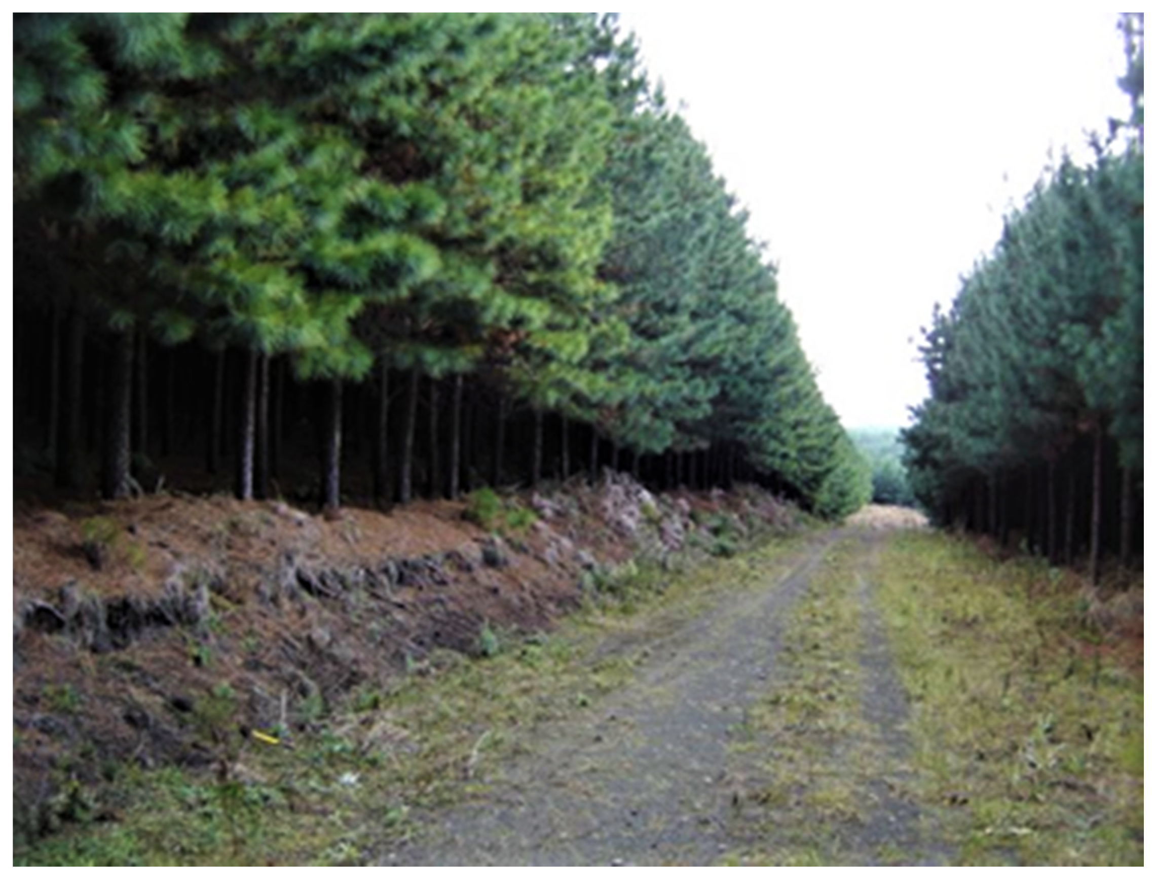
Wood samples were collected from a 10-year-old progeny trial (Figure 1) established by BattiStella in the Rio Negrinho municipality, Santa Catarina, Brazil (coordinates 26°40′07.24″ S 49°37′37.38″ W). The trial was planted in randomized blocks with 120 families, five replicates, and five plants per linear plot. Stem form, growth, and internode distribution and distance were assessed, and the best 600 trees identified for nondestructive (breast height increment cores from the best performing individuals) and destructive (breast height disc) sampling.
2.2. Sample Preparation: Radial Strips
For discs obtained from destructive sampling, pith-to-bark radial sections were cut using a bandsaw. Section dimensions were 12.5 mm longitudinally (L), and 12.5 mm tangentially (T); tree diameter determined radial (R) length. Sections were dried, glued into core holders, and cut using a twin-blade saw to give radial strips with dimensions: 2 mm (T) × 12.5 mm (L), R varied as described earlier in Section 2.2. Similar strips were prepared using the cores sampled non-destructively.
2.3. Wood Property Analysis
From the 600 samples, a subsample of 52 was available for SilviScan and NIR-HSI analysis.
2.3.1. SilviScan
SilviScan analysis was conducted at FPInnovations, Canada, on unextracted radial strips having dimensions, 2 mm tangentially, 7 mm longitudinally, with the radial dimension varying owing to variation in the diameter of trees sampled. The following wood properties were determined:
A controlled environment of 40% relative humidity and 20 °C was used for all measurements.
2.3.2. NIR-HSI Analysis
Hyperspectral images were collected using a Specim FX17 camera (wavelength range 900–1700 nm, 224 wavelengths) fitted with a Specim (OLET 17.5 F/2.1) focusing lens (Specim, Spectral Imaging Ltd., Oulu, Finland). Tungsten halogen lamps illuminated samples, while sample motion and image acquisition (which included a dark current and white reference before collecting an image of each set of samples) were controlled using Lumo software supplied with the system. Samples were analyzed on a black background, and care was taken to minimize exposure of the samples to the intense light of the lamps.
Relative reflectance values for each image was calibrated with the corresponding dark current and white reference data and then transformed to absorbance (A), where A = log10 1/R. Regions of interest (ROI), corresponding to each of the 4 samples analyzed per set, were identified, cropped, and these images averaged to give an individual spectrum per sample using MATLAB. The resultant spectra were used for the cluster analysis.
2.4. Cluster Analysis of Wood Properties Based on NIR-HSI Spectra
To group the 52 trees into groups with similar characteristics, a cluster analysis (hierarchical complete linkage with square Euclidean distance), was performed on the hyperspectral data with a matrix that consisted of 224 columns (variables–wavelengths) and 52 rows (trees) using The Unscrambler X, version 10.2 (64 bit). (Camo Software AS, Oslo, Norway). Clustering is an agglomerative method that begins by treating each sample as a single cluster and, from there, begins to group the samples based on their similarity, as measured by their square Euclidian distance, until they form a large cluster. The smaller groups, formed from the larger dataset, are known as clusters. Grouping allows identification of similar observations that can potentially categorize them. Prior to cluster analysis, the reflectance values were normalized for each wavelength by dividing by the standard deviation calculated for each wavelength. Three parameters were used to determine the final number of clusters identified. These included the cubic clustering criterion, pseudo F statistic, and pseudo t2 statistic [29]. Two and four clusters were most frequently selected, but we decided to use four as we wanted to have an indication of the most and least suitable trees, something we could not have achieved using two clusters. Prior to cluster analysis, the reflectance values were normalized for each wavelength by dividing by the standard deviation calculated for each wavelength.
2.5. Graphics
3. Results
3.1. Cluster Analysis Based on NIR Spectra
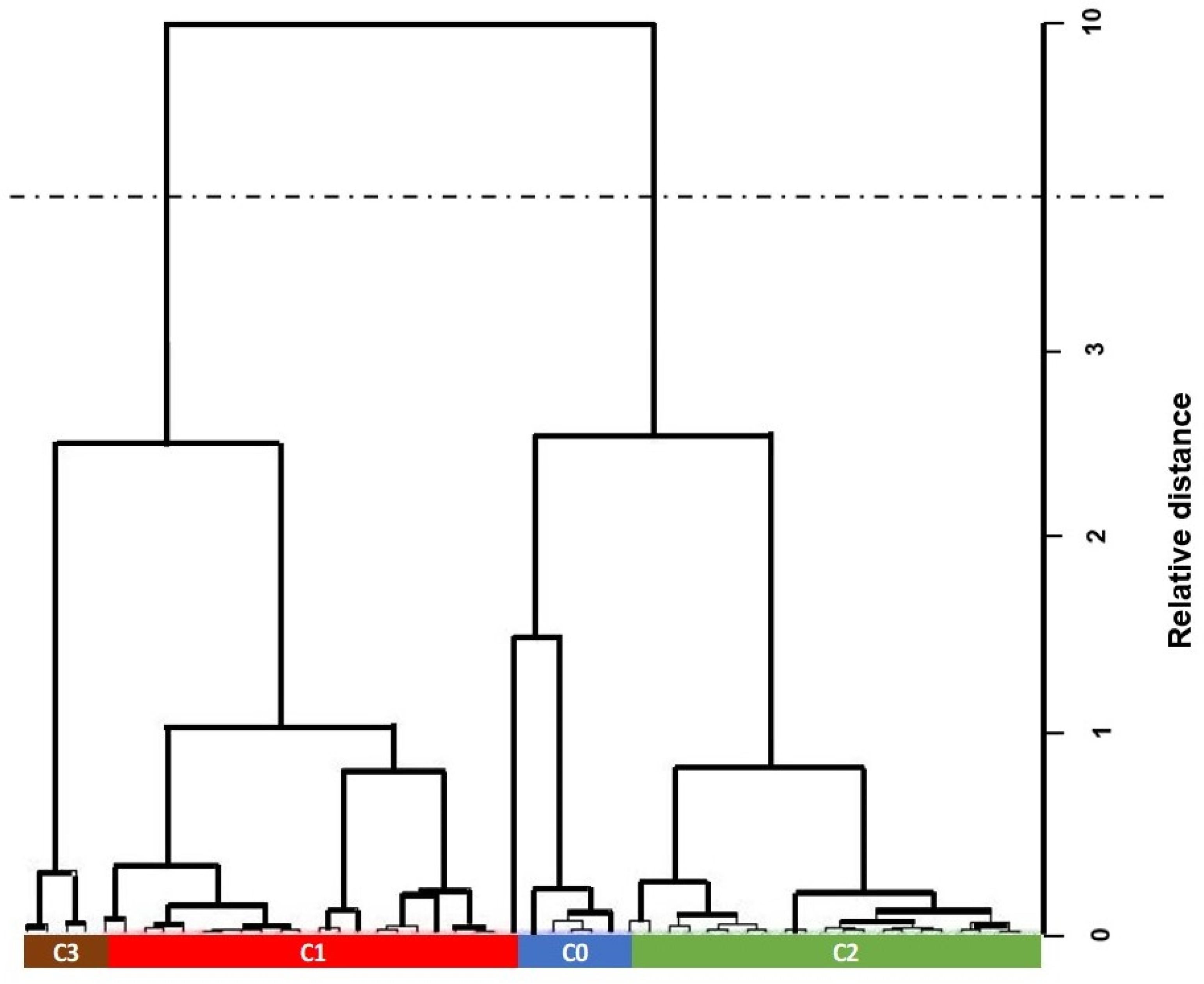
The cluster analysis using the spectral data obtained for each tree identified four groups (Figure 2). Based on each cluster, mean wood and tree growth values were determined for each measured wood property and summarized in Table 1. Cluster 0 trees (six in total) had superior wood quality having the highest mean density and stiffness. Average height (10.9 m) for Cluster 0 exceeded that of the other clusters, while the average diameter at breast height (DBH) (213 mm) was similar amongst clusters.
In terms of end-use, trees identified in Cluster 0 have the greatest potential (at age 10) for producing structural lumber. In contrast, Cluster 3, which included four trees, had the least desirable solid-wood properties, having the lowest average density and second-lowest stiffness (Cluster 2 had a lower stiffness owing to its higher MFA). Owing to low density and stiffness, trees in Cluster 3 have a lower potential for producing structural lumber and would be better suited for the manufacture of pulp or composites, such as particleboard and medium-density fiberboard. In such products, lower wood density may be beneficial in avoiding the manufacture of panels that are overly heavy, which can be problematic if density becomes too high. Clusters 1 and 2, which included the majority of trees (42), had a very similar average density, while Cluster 1 had a higher average stiffness owing to its lower MFA. These characteristics indicate that wood from these clusters may be suited to low-value solid wood applications, such as pallet stock and furniture parts. However, the characteristics of the two groups are so similar that the lower-value uses identified for both clusters could be interchanged.
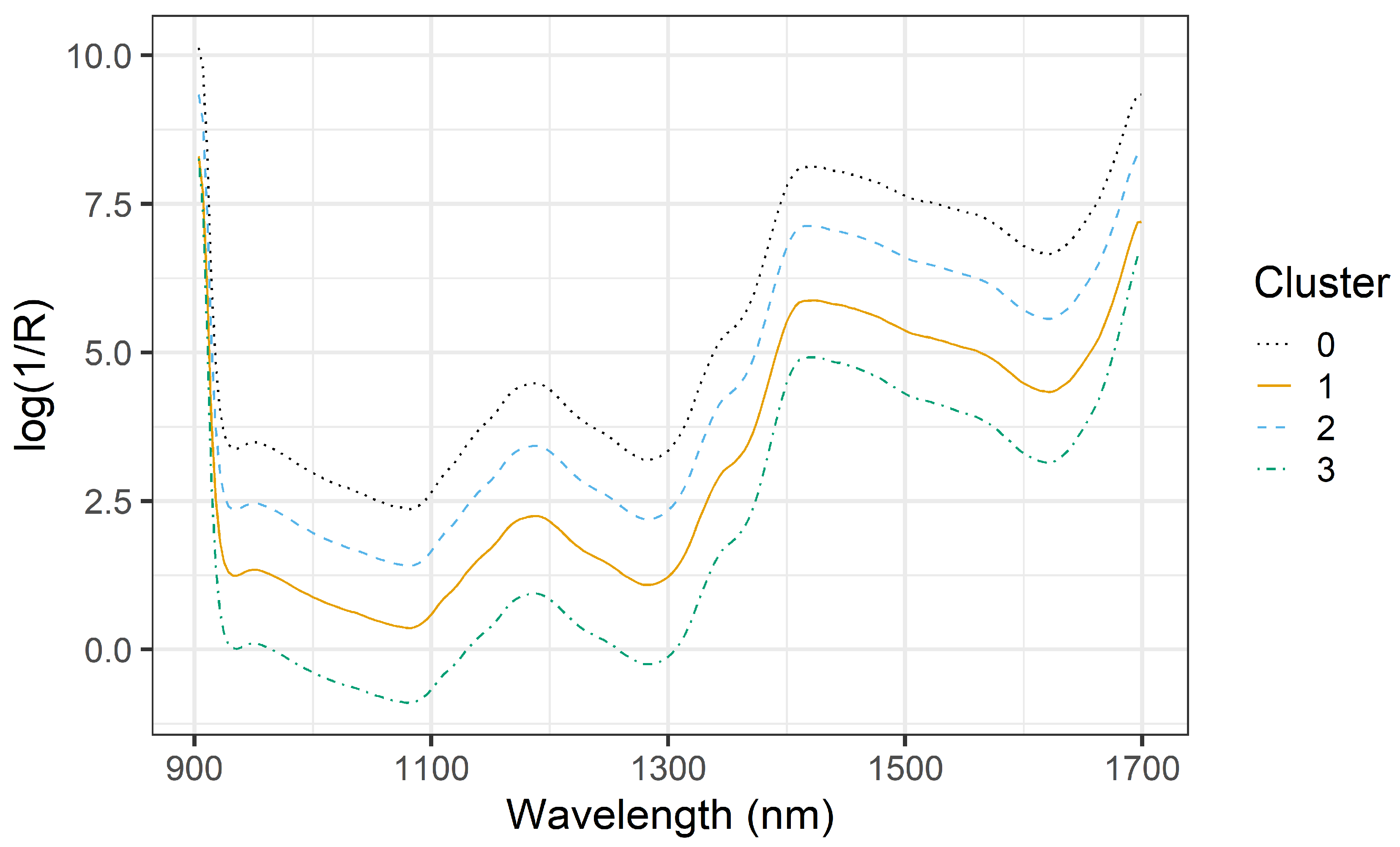
The cluster analysis relies on NIR spectra, reflecting differences in wood chemical and physical properties (no wood property information was utilized in the analysis). The average NIR spectra of each cluster show clear differences (Figure 3) with Cluster 0 trees demonstrating the largest upward baseline shift relative to the other clusters, with Cluster 3 trees having the smallest. In their study of alpine ash (Eucalyptus delegatensis R. T. Baker) solid wood samples, Schimleck et al. [34] associated such shifts with changes in wood density.
3.2. Radial Variation in Wood Properties
Ring averages based on SilviScan data were determined for each tree to examine wood property differences amongst clusters. Figure 4 (density), shows radial variation for each cluster, with fitted Loess regression lines. Based on Figure 4, trees from the two extreme clusters were clearly different in terms of average ring densities, while Clusters 1 and 2 were very similar. After ring 2, average density values for Cluster 0 were higher than the other clusters, and the difference between Cluster 0 and Clusters 1 and 2 became more pronounced as age increased. In contrast, the average ring densities of the Cluster 3 samples, with the exception of ring 1, were clearly lower than the other clusters. Despite similar initial densities (470 to 480 kg/m3), the ring averages for clusters showed different trends. Cluster 0 ring densities increased rapidly compared to the other clusters, reaching an average of 630 kg/m3 by age 9. Clusters 1 and 2 also increased, however the rate of increase was inferior to Cluster 0, and ring 9 had an average density of approximately 570 kg/m3 for both clusters. Cluster 3 trees had no change in average density (470 kg/m3) for rings 1 to 3. By ring 6, the average density was 520 kg/m3, after which little change was observed.
Direct comparisons of our density values with loblolly pine grown in the SE USA is imperfect owing to a different measure of wood density often being employed (specific gravity versus air-dry density), different sampling ages, and differences in what an estimate of average density represents. Jordan et al. [35] provide the most comprehensive study of density in loblolly pine across its natural range. However, they reported basic specific gravity (SG) values (determined from oven dry weight, green volume, and density of water), and the trees sampled were older (average age for the different physiographic regions sampled ranged from 22.4 to 24.2 years). To facilitate direct comparison, studies that utilized SilviScan to analyze loblolly pine breast height cores of similar age were identified. For example, Isik et al. [36] reported mean SilviScan density values for two sites each in Georgia aged 15 and 16 years (486 kg/m3), North Carolina aged 18 and 19 years (542 kg/m3), and South Carolina aged 14 and 15 years (499 kg/m3). These density values are similar to the average densities reported for the respective clusters in this study (Table 1), and the trees were also older. Despite the differences in age, DBH values (185 mm Georgia, 228 mm North Carolina, and 235 mm South Carolina) were similar owing to the improved growth rates of loblolly pine in southern Brazil.
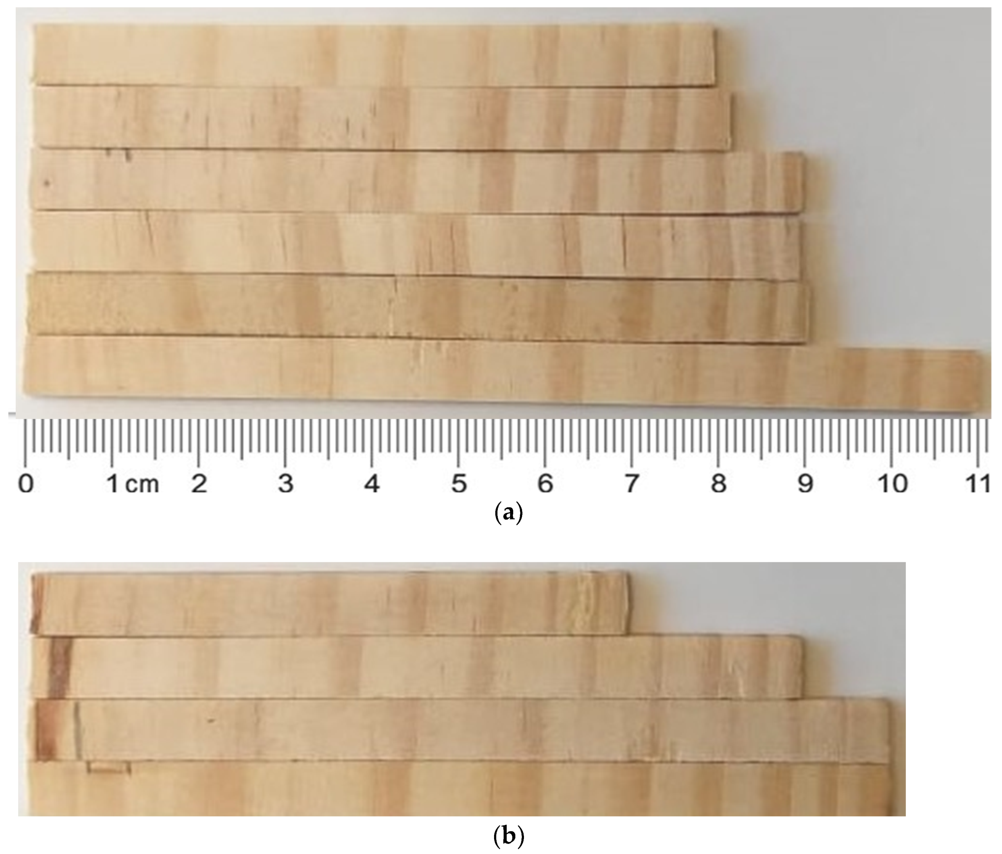
While it is not possible to compare ring densities, percent latewood (% LW) may provide useful comparative data, and, as noted by Jordan et al. [35], % LW is of critical importance in determining ring density and subsequently, whole-tree density. Jordan et al. [35] used an SG of 0.48 to separate earlywood (EW) from LW, while we used a density of 480 kg/m3 [37]. Hence, the point within a ring at which the commencement of LW production may be slightly different, but the practical significance of the difference will be small as EW changes rapidly to LW in loblolly pine [37,38]. For Cluster 0 trees, average % LW was initially low (ring 1 = 17.5%, ring 2 = 24.8%) but increased quickly (% LW for rings 6 to 8 was approximately 50%) and reached 65.3% for ring 9. In comparison, Cluster 3 had similar % LW near the pith (ring 2 = 18.1%, ring 3 = 21.3%), but it increased slowly with rings 4 to 9 having % LW in the range 26 to 34%. Clusters 1 and 2 had an initial % LW consistent with the other clusters and reached 40% LW by ring 6 and approximately 54% LW by ring 9. Pictures of the radial samples for trees in Cluster 0 and 3 are shown in Figure 5.
Figure 2 in Jordan et al. [35] indicates that % LW increases rapidly with age in the SE USA, with regional averages approaching 40% by age 5 and at least 45% by age 9 (at this age trees from stands from the south Atlantic coastal plain had 52 to 53% LW). This data indicates that % LW (and note this is on a regional basis and represents the average of many trees and sites) for trees grown in the USA south would be well above the values reported here for Cluster 3, similar to those reported for Clusters 1 and 2 and lower than those for the Cluster 0 trees.
Hart [7], in his comparison of loblolly pine grown in Santa Catarina and the USA South, observed that the ratio of EW to LW was a major difference between the two regions. On a volume basis, trees from Santa Catarina at age 17 were approximately 21 to 22% latewood, while the trees from the USA south (aged 18–21 years) had a much higher proportion (54 to 55%). When making comparisons with Hart [7], it is important to recognize that the families from the breeding trial sampled for this study are not typical of what is planted in industrial plantations. The families also represent a wide range of variability in terms of wood properties and physiology. This is apparent upon a detailed examination of the wood properties of the different clusters. The variation in % LW provides an explanation for the separation of trees into different clusters, but for trees of different families to produce such large differences in % LW while growing at the same location indicates that the trees responded very differently to the growing conditions they experienced.
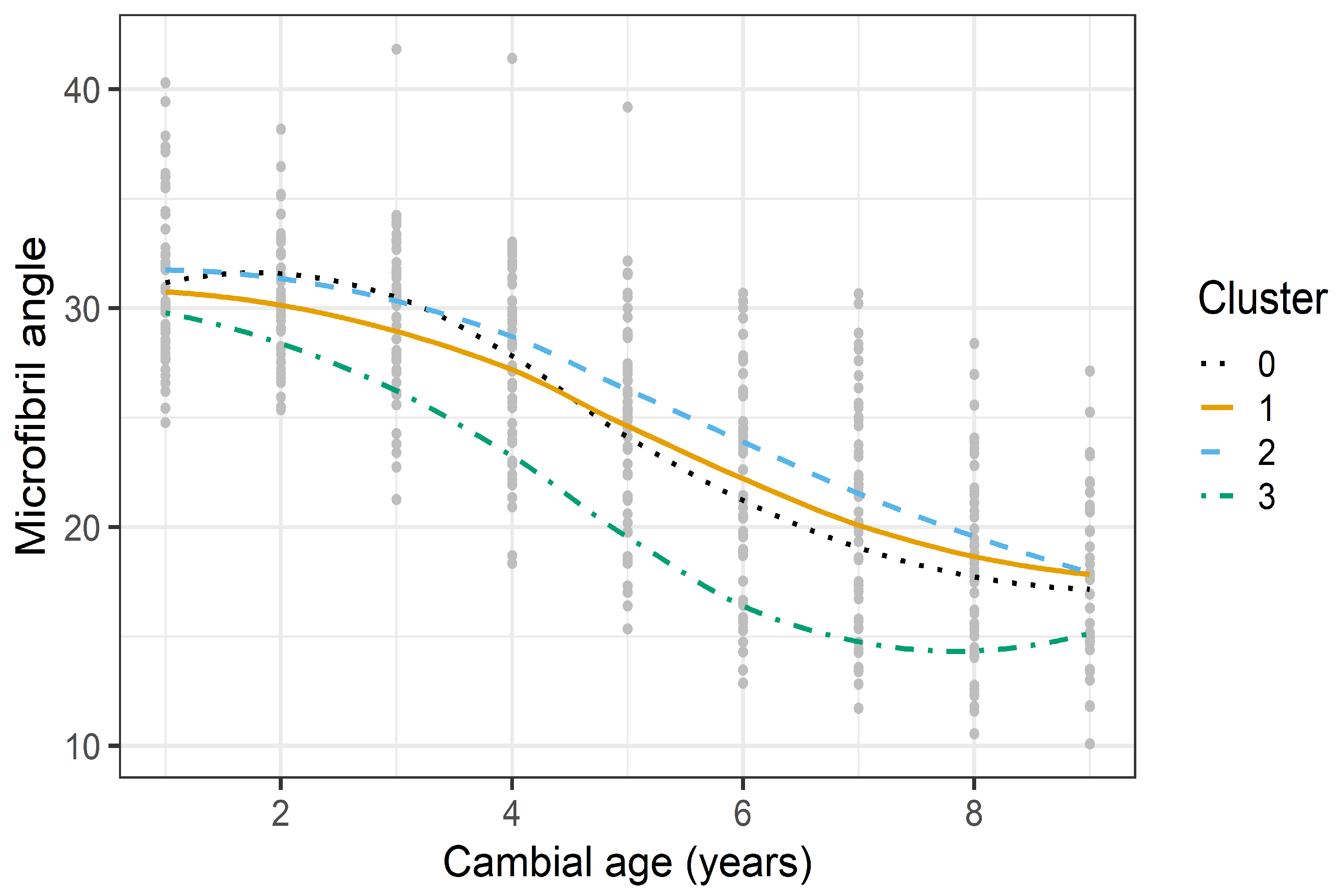
The average ring MFA of Cluster 3 was consistently lower than the other clusters (Figure 6). The MFA of ring 1 was 30°, and similar to the other clusters, but by ring 6, it had decreased to approximately 16° and was 5 to 8° lower than Clusters 0 to 2. By ring 9, Clusters 0 to 2, which demonstrated similar radial trends of decreasing MFA, had similar angles (18°) and close to that of Cluster 3 (16°). Three samples (one each in rings 3 to 5) with MFAs close to or above 40° were much higher than the other values observed for these rings, and likely indicate the presence of compression wood in one tree.
MFA variation for loblolly pine grown in the SE USA is not as extensively studied as density (or SG) owing to the cost of analysis. Jordan et al. [39] and Jordan et al. [40] reported MFA within-tree variation for a small number of trees from five physiographic regions (the upper coastal plain was not represented). Jordan et al. [40] reported average MFAs near the pith of approximately 35° for trees from the north Atlantic coastal plain and Piedmont, whereas MFA for the other regions was closer to 30°. For all regions in the SE USA, MFA decreased rapidly in the first few years of growth, and at age 10, trees from the north Atlantic coastal plain and Piedmont had the highest average breast height MFAs (approximately 23°), whereas MFAs for the remaining three regions (hilly, gulf, and south Atlantic coastal plains) were all similar (16 to 17°).
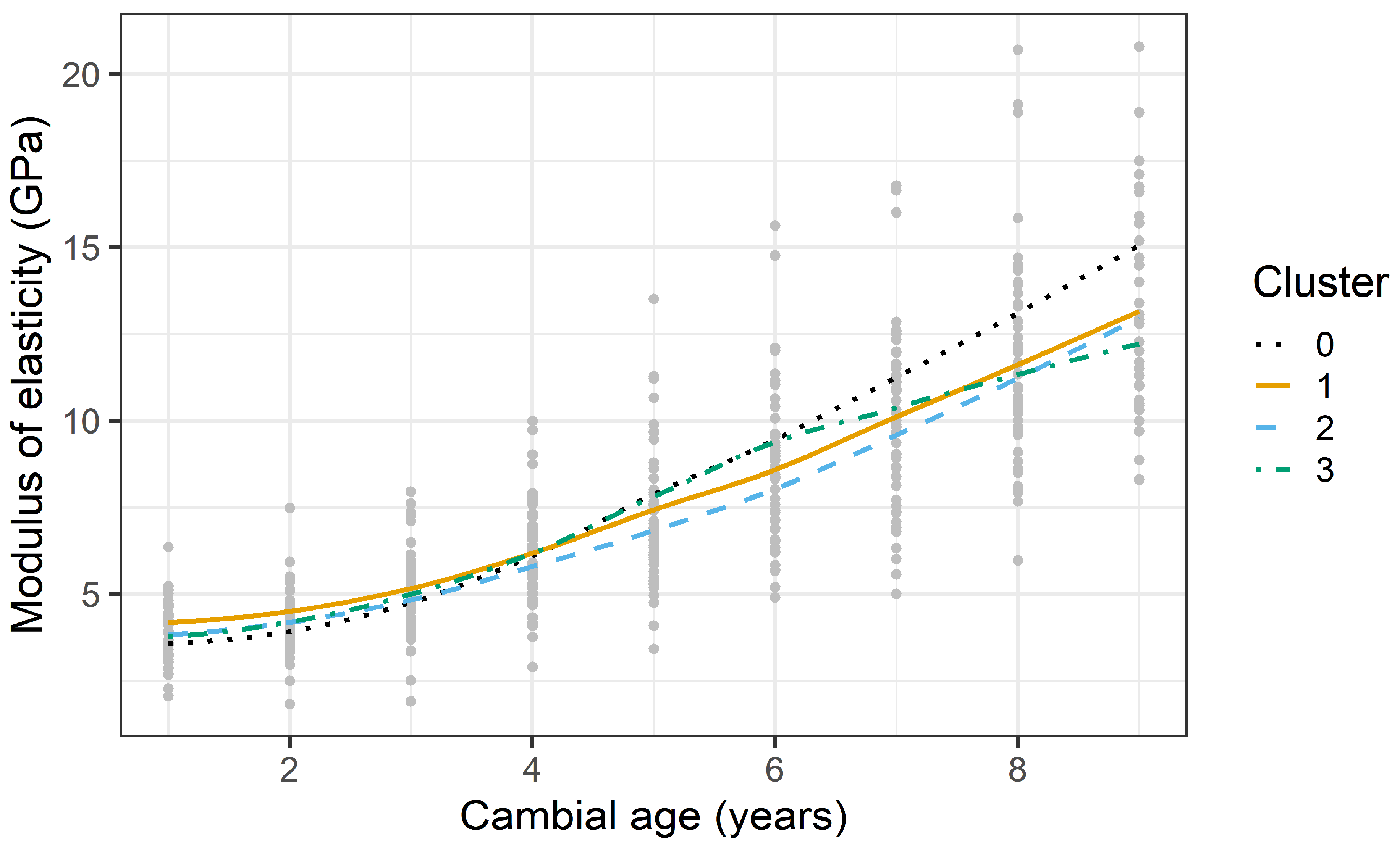
Radial variation in stiffness (Figure 7) was similar across clusters. Stiffness of rings 1 to 3 for all clusters was very low (5 GPa or less) but increased rapidly and by ring 7, averaged 10 GPa. Trees in Cluster 0 had the highest ring 7 stiffness with differences between it and the other clusters becoming more pronounced as the trees grew older. By Ring 9, average stiffness for the Cluster 0 trees was 15 GPa compared to approximately 12.5 GPa for the other 3 clusters. The marked increase in stiffness for Cluster 0 can be related to the higher density of this cluster (Figure 4) and a decreasing trend in MFA particularly after ring 5 when its average ring MFA became, and stayed, lower than the MFA of Clusters 1 and 2 (Figure 6). The comparatively high stiffness of trees in Cluster 3 up until ring 6 relates directly to the lower initial MFAs of this cluster. After ring 6, differences in MFA became progressively smaller with age, and while Cluster 3 trees still had the lowest ring MFAs (Figure 6), their lower ring densities (Figure 4) resulted in stiffness increasing at a slower rate than for Clusters 0 to 2. It is also apparent in Figure 7 that a small number of trees have quite high ring stiffness values for rings 8 and 9, with stiffness values being close to 20 GPa.
Antony et al. [41] reported stiffness values for the same regions examined by Jordan et al. [35]. Corewood stiffness values for static bending samples from a height of 2.4 m ranged from 3.6 GPa (North Atlantic coastal plain) to 5.6 GPa (gulf coastal plain), while outerwood stiffness ranged from 8 GPa (North Atlantic coastal plain) to 10.9 GPa (gulf coastal plain). The stiffness averages for the different clusters (Table 1) are comparable to the corewood averages reported by Antony et al. [41]. However, it is important to note that the corewood samples examined by Antony et al. [41] generally represented rings two to four. Antony et al. [40] also measured stiffness on short, clear bending specimens (static stiffness) versus the dynamic stiffness used here. Jordan et al. [35] observed that outerwood production commences in loblolly pine by year 13 in the SE USA. Hence, the trees examined in this study (aged 10 years) largely comprise corewood.
We have shown that within a Brazilian-grown loblolly pine progeny test, it is possible to use NIR-HSI data to identify groups (or clusters) of trees. Our hypothesis was that clusters would differ in terms of their wood properties and SilviScan data for density, MFA, and stiffness when averaged for trees within clusters, confirmed wood property differences among clusters. Four clusters were identified, with trees identified in Clusters 0 and 3 having the highest and lowest average densities, respectively. Clusters 1 and 2 had very similar average wood properties, with densities closer to that of Cluster 0 than Cluster 3. Radial trends of increasing density and stiffness and decreasing MFA observed for the clusters are consistent with trends reported for loblolly pine [7,35,41,42]. The greatest differences in trends amongst clusters were observed for density (clearly highest for Cluster 0 and lowest for Cluster 3) and MFA (clearly lowest for Cluster 3). The higher densities for Cluster 0 were related to a higher % LW compared to the other clusters, with Cluster 3 having the lowest.
NIR-HSI provides a rapid approach for collecting wood property data and, when coupled with cluster analysis, potentially allows screening for desirable wood properties amongst families in tree improvement programs. Selection will be company-specific, with emphasis likely to be on improving solid wood properties. Hence, as an initial screening (based on NIR-HSI cluster analysis and supported by corresponding SilviScan data), trees in Cluster 0 would be likely candidates for further evaluation and testing. Regardless of the target of the breeding program, NIR-HSI can focus effort on trees with desirable properties. The greater provision of wood property data would allow tree breeders to have the option of selecting fewer families for field experiments, or they could decide which families in existing trials would be the most suitable for meeting the objectives of a company investing in commercial plantations on a large-scale. It also provides a rapid approach for collecting wood property-related data from increment cores or discs. The same outcome could likely be achieved using a standard NIR spectrometer [11,12,13] where spectra at a given spatial resolution are collected and then averaged, but the time required to collect data is greatly reduced using a NIR-HSI system.
4. Conclusions
Near-infrared hyperspectral images (NIR-HSI) were collected from 52 radial strips obtained from a 10-year-old loblolly pine progeny trial located in Brazil. The NIR data were subject to a hierarchical complete linkage with square Euclidean distance cluster analysis. Four clusters (0, 1, 2, 3) were identified, and we demonstrated that clusters differed in terms of average air-dry density, microfibril angle (MFA), and stiffness. Average ring data were used to compare clusters, and Cluster 0 trees had the highest average ring densities, whereas those in Cluster 3, the lowest. Cluster 3 trees also had the lowest ring MFAs.
Author Contributions
Conceptualization, A.H., J.L.M.M., and L.S.; methodology, A.H., J.L.M.M., and L.S.; sample collection and preparation, J.G.P. and R.T.; software, L.S., J.L.M.M., and J.D.; formal analysis, L.S., J.L.M.M., and J.D.; resources, J.L.M.M. and A.H.; data curation, J.L.M.M.; writing—original draft preparation, L.S. and J.L.M.M.; writing—review and editing, L.S., J.L.M.M., and J.D.; visualization, J.L.M.M. and J.D.; supervision, J.L.M.M.; project administration, J.L.M.M.; funding acquisition, J.L.M.M. and A.H. All authors have read and agreed to the published version of the manuscript.
Funding
National Council for Scientific and Technological Development-CNPq for granting support for the execution of the research project. FINEP for the grant to develop the project “Use of biotechnological tools to improve the genetic quality of Pinus taeda and alternatives species”.
Acknowledgments
Battistella Florestal for the establishment, maintenance, and data and sample collection from the progeny test located in the Rio Negrinho municipality of Santa Catarina, Brazil. Oregon State University, College of Forestry for Hosting J.M., and Marja Haagsma and Gerald Page (Oregon State University) for their MATLAB expertise.
Conflicts of Interest
The authors declare no conflict of interest.
References
- Payn, T.; Carnus, J.-M.; Freer-Smith, P.; Kimberley, M.; Kollert, W.; Liu, S.; Orazio, C.; Rodriguez, L.; Silva, L.N.; Wingfield, M.J. Changes in planted forests and future global implications. For. Ecol. Manag. 2015, 352, 57–67. [Google Scholar] [CrossRef] [Green Version]
- IBA. Indústria Brasileira de Árvores, 2019 Report; IBA: São Paulo, Brazil, 2019; p. 80. [Google Scholar]
- Ferreira, A.R. Análise Genética E Seleção Em Testes Dialélicos De Pinus taeda L. Ph.D. Thesis, Universidade Federal do Paraná, Curitiba, Brazil, 2005; p. 196. [Google Scholar]
- De Melo Sixel, R.M.; Junior, J.C.A.; de Moraes Goncalves, J.L.; Alvares, C.A.; Andrade, G.R.P.; Azevado, A.C.; Stahl, J.; Moreira, A.M. Sustainability of wood productivity of Pinus taeda based on nutrient export and stocks in the biomass and in the soil. R. Bras. Ci. Solo 2015, 39, 1416–1427. [Google Scholar] [CrossRef] [Green Version]
- Fox, T.R.; Jokela, E.J.; Allen, H.L. The development of pine plantation silviculture in the southern United States. J. For. 2007, 105, 337–347. [Google Scholar]
- Aspinwall, M.J.; McKeand, S.E.; King, J.S. Carbon sequestration from 40 years of planting genetically improved loblolly pine across the southeast United States. For. Sci. 2012, 58, 446–546. [Google Scholar] [CrossRef]
- Hart, P.W. Differences in juvenile Pinus taeda (loblolly pine) grown in Santa Catarina, Brazil and the southern United States. In Proceedings of the TAPPI Engineering, Pulping and Environmental Conference, Memphis, TN, USA, 11–14 October 2009. [Google Scholar]
- Moore, J.R.; Cown, D.J. Corewood (Juvenile Wood) and its impact on wood utilisation. Curr. For. Rep. 2017, 3, 107–118. [Google Scholar] [CrossRef]
- Higa, A.R.; Kageyama, P.Y.; Ferreira, M. Variação da densidade básica da madeira de Pinus elliottii e P. Taeda. IPEF Piracicaba 1973, 7, 79. [Google Scholar]
- Schimleck, L.; Apiolaza, L.; Dahlen, J.; Downes, G.; Emms, G.; Evans, R.; Moore, J.; Pâques, L.; Van den Bulcke, J.; Wang, X. Non-destructive evaluation techniques and what they tell us about wood property variation. Forests 2019, 10, 728. [Google Scholar] [CrossRef] [Green Version]
- Jones, P.D.; Schimleck, L.R.; Peter, G.F.; Daniels, R.F.; Clark, A. Nondestructive estimation of Pinus taeda L. wood properties for samples from a wide range of sites in Georgia. Can. J. For. Res. 2005, 35, 85–92. [Google Scholar] [CrossRef] [Green Version]
- Downes, G.M.; Meder, R.; Ebdon, N.; Bond, H.; Evans, R.; Joyce, K.; Southerton, S. Radial variation in cellulose content and Kraft pulp yield in Eucalyptus nitens using near-infrared spectral analysis of air-dry wood surfaces. J. Near Infrared Spectrosc. 2010, 18, 147–155. [Google Scholar] [CrossRef]
- Meder, R.; Marston, D.; Ebdon, N.; Evans, R. Spatially-resolved radial scanning of tree increment cores for near infrared prediction of microfibril angle and chemical composition. J. Near Infrared Spectrosc. 2010, 18, 499–505. [Google Scholar] [CrossRef]
- Burger, J.; Gowen, A. Data handling in hyperspectral image analysis. Chemom. Intell. Lab. Syst. 2011, 108, 13–22. [Google Scholar] [CrossRef]
- Manley, M. Near-infrared spectroscopy and hyperspectral imaging: Non-destructive analysis of biological materials. Chem. Soc. Rev. 2014, 43, 8200–8214. [Google Scholar] [CrossRef] [Green Version]
- Mishra, P.; Asaari, M.S.M.; Herrero-Langreo, A.; Lohumi, S.; Diezma, B.; Scheunders, P. Close range hyperspectral imaging of plants: A review. Biosyst. Eng. 2017, 164, 49–67. [Google Scholar] [CrossRef]
- Thumm, A.; Riddell, M.; Nanayakkara, B.; Harrington, J.; Meder, R. Near infrared hyperspectral imaging applied to mapping chemical composition in wood samples. J. Near Infrared Spectrosc. 2010, 18, 507–515. [Google Scholar] [CrossRef]
- Thumm, A.; Riddell, M.; Nanayakkara, B.; Harrington, J.; Meder, R. Mapping within-stem variation of chemical composition by near infrared hyperspectral imaging. J. Near Infrared Spectrosc. 2016, 24, 605–616. [Google Scholar] [CrossRef]
- Ma, T.; Inagaki, T.; Tsuchikawa, S. Calibration of SilviScan data of Cryptomeria japonica wood concerning density and microfibril angles with NIR hyperspectral imaging with high spatial resolution. Holzforschung 2017, 71, 341–347. [Google Scholar] [CrossRef]
- Ma, T.; Inagaki, T.; Tsuchikawa, S. Non-destructive evaluation of wood stiffness and fiber coarseness, derived from SilviScan data, via near infrared hyperspectral imaging. J. Near Infrared Spectrosc. 2018, 26, 398–405. [Google Scholar] [CrossRef]
- Haddadi, A.; Burger, J.; Leblon, B.; Pirouz, Z.; Groves, K.; Nader, J. Using near-infrared hyperspectral images on subalpine fire board. Part 1: Moisture content estimation. Wood Mater. Sci. Eng. 2015, 10, 27–40. [Google Scholar] [CrossRef]
- Haddadi, A.; Burger, J.; Leblon, B.; Pirouz, Z.; Groves, K.; Nader, J. Using near-infrared hyperspectral images on subalpine fire board. Part 2: Density and basic specific gravity estimation. Wood Mater. Sci. Eng. 2015, 10, 41–56. [Google Scholar] [CrossRef]
- Meder, R.; Meglen, R.R. Near infrared spectroscopic and hyperspectral imaging of compression wood in Pinus radiata D. Don. J. Near Infrared Spectrosc. 2012, 20, 583–589. [Google Scholar] [CrossRef]
- Thumm, A.; Riddell, M. Resin defect detection in appearance lumber using 2D NIR spectroscopy. Eur. J. Wood Wood Prod. 2017, 75, 995–1002. [Google Scholar] [CrossRef]
- Evans, R. Rapid scanning of microfibril angle in increment cores by x ray diffractometry. In Proceedings of the IAWA/IUFRO International Workshop on the Significance of Microfibril Angle to Wood Quality, Westport, New Zealand, 21–25 November 1997. [Google Scholar]
- Evans, R. Rapid Measurement of the transverse dimensions of tracheids in radial wood sections from Pinus radiata. Holzforschung 1994, 48, 168–172. [Google Scholar] [CrossRef]
- Evans, R. A variance approach to the X-ray dffractometric estimation of microfibril angle in wood. Appita J. 1999, 52, 283–289. [Google Scholar]
- Evans, R. Wood stiffness by X-ray diffractometry. In Characterisation of the Cellulosic Cell Wall; Stokke, D., Groom, L., Eds.; Blackwell Publishing: Ames, IA, USA, 2006; pp. 138–146. [Google Scholar]
- SAS Institute Inc. SAS/STAT® 13.1 User’s Guide; SAS Institute Inc.: Cary, NC, USA, 2013. [Google Scholar]
- R Core Team. R: A Language and Environment for Statistical Computing; R Foundation for Statistical Computing: Vienna, Austria, 2020; Available online: http://www.R-project.org/ (accessed on 5 May 2020).
- RStudio. RStudio: Integrated Development Environment for R; RStudio Inc.: Boston, MA, USA, 2020; Available online: https://www.rstudio.com/ (accessed on 5 May 2020).
- Wickham, H. Ggplot2: Elegant Graphics for Data Analysis; Springer: New York, NY, USA, 2009. [Google Scholar]
- Wickham, H. Tidyverse. R Package Version 1.3.0. 2019. Available online: https://CRAN.R-project.org/package=tidyverse (accessed on 5 May 2020).
- Schimleck, L.R.; Evans, R.; Ilic, J. Estimation of Eucalyptus delegatensis clear wood properties by near infrared spectroscopy. Can. J. For. Res. 2001, 31, 1671–1675. [Google Scholar] [CrossRef]
- Jordan, L.; Clark, A.; Schimleck, L.R.; Hall, D.B.; Daniels, R.F. Regional variation in wood specific gravity of planted loblolly pine in the United States. Can. J. For. Res. 2008, 38, 698–710. [Google Scholar] [CrossRef]
- Isik, F.; Mora, C.; Schimleck, L.R. Genetic variation in Pinus taeda wood properties predicted using non-destructive techniques. Ann. For. Sci. 2011, 68, 283–293. [Google Scholar] [CrossRef] [Green Version]
- Antony, F.; Schimleck, L.R.; Daniels, R.F. A comparison of earlywood-latewood demarcation methods within an annual ring—A case study in loblolly pine. IAWA J. 2012, 33, 187–195. [Google Scholar] [CrossRef]
- Eberhardt, T.L.; Samuelson, L. Collection of wood quality data by X-ray densitometry: A case study with three southern pines. Wood Sci. Technol. 2015, 49, 739–753. [Google Scholar] [CrossRef]
- Jordan, L.; He, R.C.; Hall, D.B.; Clark, A.; Daniels, R.F. Variation in loblolly pine cross-sectional microfibril angle with tree height and physiographic region. Wood Fiber Sci. 2006, 38, 390–398. [Google Scholar]
- Jordan, L.; He, R.C.; Hall, D.B.; Clark, A.; Daniels, R.F. Variation in loblolly pine ring microfibril angle in the Southeastern United States. Wood Fiber Sci. 2007, 39, 352–363. [Google Scholar]
- Antony, F.; Jordan, L.; Schimleck, L.R.; Clark, A.; Souter, R.A.; Daniels, R.F. Regional variation in wood modulus of elasticity (stiffness) and modulus of rupture (strength) of planted loblolly pine in the United States. Can. J. For. Res. 2011, 41, 1522–1533. [Google Scholar] [CrossRef]
- Burdon, R.D.; Kibblewhite, R.P.; Walker, J.C.F.; Megraw, R.A.; Evans, R.; Cown, D.J. Juvenile versus mature wood: A new concept, orthogonal to corewood versus outerwood, with special reference to Pinus radiata and P. Taeda. For. Sci. 2004, 50, 399–415. [Google Scholar]
Figure 1.
BattiStella loblolly pine at age 10 in the Rio Negrinho municipality of Santa Catarina, Brazil.
Figure 1.
BattiStella loblolly pine at age 10 in the Rio Negrinho municipality of Santa Catarina, Brazil.

Figure 2.
Trees determined to have similar wood properties based on complete linkage clustering with square Euclidian distance of near-infrared (NIR) spectral data.
Figure 2.
Trees determined to have similar wood properties based on complete linkage clustering with square Euclidian distance of near-infrared (NIR) spectral data.

Figure 3.
Average NIR spectra for each cluster.

Figure 4.
Density radial variation for trees representing the average wood property values of each cluster.
Figure 4.
Density radial variation for trees representing the average wood property values of each cluster.

Figure 5.
Radial strips for (a) Cluster 0 and (b) Cluster 3 trees.

Figure 6.
Microfibril angle (MFA) radial variation for trees representing the average wood property values of each cluster.
Figure 6.
Microfibril angle (MFA) radial variation for trees representing the average wood property values of each cluster.

Figure 7.
Stiffness radial variation for trees representing the average wood property values of each cluster.
Figure 7.
Stiffness radial variation for trees representing the average wood property values of each cluster.


Table 1.
Cluster means, standard deviations, and median values (in italics) for SilviScan determined wood properties (density, microfibril angle (MFA) and stiffness) and tree height and diameter at breast height (DBH).
Table 1.
Cluster means, standard deviations, and median values (in italics) for SilviScan determined wood properties (density, microfibril angle (MFA) and stiffness) and tree height and diameter at breast height (DBH).
| Density (kg/m3) | MFA (deg.) | Stiffness (GPa) | Average Tree height 1 (m) | Average Tree DBH (mm) | |
|---|---|---|---|---|---|
| Cluster 0 (6 trees) | 546.8, 51.7 550.8 | 24.9, 7.2 27.2 | 7.9, 4.6 6.3 | 10.9, 1.0 11.2 | 213, 6.2 213 |
| Cluster 1 (21 trees) | 520.0, 63.8 522.8 | 24.5, 6.4 25.4 | 7.7, 3.6 6.9 | 10.3, 1.3 10.5 | 216, 25.4 221 |
| Cluster 2 (21 trees) | 524.5, 61.5 522.0 | 25.9, 6.3 26.6 | 7.2, 3.3 6.6 | 9.8, 1.0 9.6 | 212, 20.1 217 |
| Cluster 3 (4 trees) | 493.6, 39.7 487.4 | 21.2, 6.6 21.3 | 7.5, 3.4 6.7 | 9.5, 1.5 9.0 | 211, 36.1 217 |
1 Tree height was measured to a diameter of 80 mm (minimum for wood product manufacturing).
© 2020 by the authors. Licensee MDPI, Basel, Switzerland. This article is an open access article distributed under the terms and conditions of the Creative Commons Attribution (CC BY) license (http://creativecommons.org/licenses/by/4.0/).
Share and Cite
MDPI and ACS Style
Schimleck, L.; Matos, J.L.M.; Higa, A.; Trianoski, R.; Prata, J.G.; Dahlen, J. Classifying Wood Properties of Loblolly Pine Grown in Southern Brazil Using NIR-Hyperspectral Imaging. Forests 2020, 11, 686. https://doi.org/10.3390/f11060686
AMA Style
Schimleck L, Matos JLM, Higa A, Trianoski R, Prata JG, Dahlen J. Classifying Wood Properties of Loblolly Pine Grown in Southern Brazil Using NIR-Hyperspectral Imaging. Forests. 2020; 11(6):686. https://doi.org/10.3390/f11060686
Chicago/Turabian StyleSchimleck, Laurence, Jorge L. M. Matos, Antonio Higa, Rosilani Trianoski, José G. Prata, and Joseph Dahlen. 2020. "Classifying Wood Properties of Loblolly Pine Grown in Southern Brazil Using NIR-Hyperspectral Imaging" Forests 11, no. 6: 686. https://doi.org/10.3390/f11060686
Note that from the first issue of 2016, this journal uses article numbers instead of page numbers. See further details here.