
Abstract
Polymer nanocomposites as dielectrics have attracted a wide range of research interests due to their improved performance. One of the observed characteristics of polymer nanocomposites is the suppression on space charge injection and accumulation and the charge transport mechanism behind is also investigated based on thermally activated hopping (TAH) and quantum mechanical tunnelling (QMT) mechanisms. However, there still lacks research on the effect of moisture on charge transport characteristics and its relationship with experimental results. We herein proposed a method to re-virtualize the distribution of nanoparticles/their aggregates based on the multidimensional scaling method in the first step, and a simple numerical method is further following to estimate the contribution of TAH and QMT conductivities to the experimental ones. The results, firstly, indicate the presence of moisture could lead to significant charge injections, and for different relative humidity conditions, due to their diverse water shell thickness, the separation distances of nanoparticles where deep/shallow traps locate show an obvious reduction and consequently vary the contribution of TAH and QMT conductivities in the measured ones. Second, the TAH mechanism plays the main role in charge transport/conduction, especially under lower RH conditions, while the obvious increment of QMT conduction is attributed to the reduced trap distances caused by thicker conductive water shells and support the existence of deep traps. Besides, the proposed model could be potentially extended to other research topics on electrical properties of polymer nanocomposites, such as particle size, dispersion/distribution status and filler loading concentrations which can be reflected and explained via the variation of nanoparticle surface/trap site distances.
Export citation and abstract BibTeX RIS

Original content from this work may be used under the terms of the Creative Commons Attribution 4.0 license. Any further distribution of this work must maintain attribution to the author(s) and the title of the work, journal citation and DOI.
1. Introduction
Nanodielectrics have attracted a lot of research over the last two decades [1, 2], As nanoparticles (NPs) have unique characteristics due to their large specific surface areas [3, 4] and various functional surface chemistries [5], they have a potential to reinforce dielectric properties of polymer matrices and some research has shown the enhancement at the low filler loading ratios (normally <5 wt%) [6]. 'Trap sites' is usually used as a term to explain the charge dynamics and conduction within polymer nanocomposites. Earlier studies have also found that charge trapping and detrapping determine the charge transport in the materials [7, 8], and the mechanism of within nanocomposites under an external electric field has also been well investigated [9, 10]. There are two mechanisms that are considered mainly contributing to the charge transport in bulk of the material [11]. One is known as thermally activated hopping (TAH) as shown in figure 1(a), where the electron/hole gained sufficient energy via thermal fluctuations could overcome the potential barrier to hop from one trap to another. In the case of the hopping process, TAH conductivity (σTAH) can be expressed by following equation (1) [12]:
where E is the applied electric field, T is the absolute temperature, qe is the elementary electron, Et is the trap energy or barrier height, kB is the Boltzmann constant, N is the concentration of carrier, υTAH is the frequency of hopping and dTAH is the average separation distance for the TAH. Another mechanism is quantum mechanical tunnelling (QMT), seen in figure 1(a), by that an electron/hole can move from one trap to a close adjacent one, as an electron can tunnel through narrow barriers in a waveform and simply 'appears' into a nearby trap [13]. Equation (2) shows the conductivity by the QMT mechanism [9]:
where N' is the energy density of trap states, υQMT is the frequency of tunnelling, dQMT is the separation distance of traps related to the tunnelling effect between two adjacent traps in the field direction, the functions ZV1 and ZV2 are complex polynomial functions of T and β (additional information about these functions can be found in [9]). Some researchers have reported various threshold distances between traps of tunnelling, and one has quantified it as ∼10 nm [14] whilst dTAH could be much larger [9]. Thus, it can be noticed that both σTAH and σQMT will be strongly influenced by the concentration of traps sites. Moreover, the presence of NPs could introduce shallow [15] and deep traps around [10], and the latter is closer to the particle surface due to the chemical bonding and reported to suppress the charge injection and movement [6]. In some previous research, the tunnelling process is suggested to occur within deep traps and explain charge transport in polymer nanocomposites in polymer nanocomposites of higher filler concentrations [9], indicating that the separation distance between two adjacent NPs is an essential factor to influence charge dynamics and conduction behaviours in the system. There is also some literature reporting an increase in direct current (DC) conductivity after adding nanofillers, which is more pronounced in samples of higher filler loading ratios due to decreased inter-particle distance and agglomerations [16].

Figure 1. (a) Charge transport within two spherical nanoparticles; (b) two-layer structure of 'water shell' around spherical nanoparticles and potential impact on charge transport: 1st tightly bonded water shell formed due to surface hydrophilic groups; 2nd water shell loosely interacted with the first layer by Van der Waals forces or located in the free volumes in the interphase [18].
Download figure:
Standard image High-resolution imageThe addition of NPs could also exacerbate the water absorption in some polymer matrices or even lead to the formation of a conductive phase around the NP depicted as 'water shells' which is firstly proposed by Zou et al [17], as illustrated in figure 1(b). This is a combined consequence of free volume in the polymer-particle interphase and hydroxyl groups on the surface of NPs, which has been demonstrated in our previous research [18]. Hui et al hypothesized the formation of water shells surrounding the particles and consequent changes in the inter-particle/aggregate distances are two major factors affecting the percolation of silica-based nanocomposites [16], leading to the higher mobility of charge carriers (as illustrated in figure 1(b)) and resultant worse dielectric properties [19, 20].
Therefore, in this paper, we will, first, propose a model to reconstruct the nanoparticle dispersion and distribution in the polymer nanocomposites and then numerically estimate the relationship between the formation of 'water shell' and charge transport characteristics.
2. Experiment preparation
2.1. Materials and sample conditioning
The polymer nanocomposite system in this work composes of epoxy resin as a matrix and nanosilica particles as fillers. The former is a bisphenol-A diglycidyl ether (D.E.R. 332, density 1.16 g cm−3) cured with polyether amine hardener (\hbox{Jeffamine} D-230, density 0.948 g cm−3) supplied by Huntsman, and the latter are commercially available as-received spherical nano-SiO2 fillers provided by Sigma–Aldrich. The average particle size (APS) based on the B.E.T. measuring method is 10–20 nm. Nanocomposite samples were cured at 393 K for 4 h following the same procedures in our previous work [18], and controlled in the vacuum oven (103 Pa, 333 K) for 72 h and then stored in the vacuum desiccator with dried silica gel at 293 K before tests. The filler loading ratio is 3 wt% and the sample is coded as EPS3: EP for epoxy resin, S for untreated nanosilica composites and the number represents the filler loading.
Samples were conditioned under three kinds of relative humidity (RH) conditions at 293 K:
- All dry samples were held in the vacuum oven (103 Pa, 333 K, for 72 h) and then stored in a vacuum desiccator with dried silica gel.
- 60% RH: These samples were stored in a RH controlled chamber, where actual RH is in the range from 56% to 62%.
- Saturated: These samples were immersed in de-ionised water for 10 d before testing.
All the samples were held in their respective environments and it took about 10 d until the weight of samples become stable under conditions with moistures.
2.2. Characterisation methods
EVO® 50 scanning electron microscopy (SEM) was used to capture the morphology images of epoxy nanocomposites. The gun voltage was set to 15 kV at the working distance ca. 7 mm. All samples have been coated with gold before the test by the Emitech K550X sputter coater at 25 mA for 3 min.
DC conductivity measurements were carried out on samples that were pre-conditioned in different humidity environments. Thin-film samples with a thickness of ca. (145 ± 10) µm were sputter-coated with gold with a diameter of 30 mm and then placed between two parallel electrodes (20 mm in diameter) and a voltage between 5 and 6 kV was applied in order to achieve an average electric field of (AEF) ∼40 kV mm−1 inside the sample. A Keithley® 6487 pico-ammeter was used to measure the current through the same film specimen as a function of time, DC conductivity (σm) was then calculated and recorded at room temperature under ambient RH conditions.
'Volts-on' measurements were taken in the experiments by a PEA technique implemented in our previous work [20], meaning that readings will be taken by applying a pulse when a voltage is applied to the samples. The applied voltage during the volts-on measurements is ∼5 to 6 kV for an AEF at 40 kV mm−1, and data were recorded periodically.
3. Quantification method and particle/aggregate distribution reconstruction modelling
3.1. Quantification
One of the SEM images of EPS3 is shown in figure 2. A previously proposed quantification method was used to generate quantitative data of how nanosilica particles were dispersed and distributed in the epoxy matrix which are two aspects to figure out the mixing state of NPs [21]: the first is the dispersion of particles, relating to the size reduction of the agglomerations of particles; the second is the distribution of particles/aggregates, involving the distribution state of particles/aggregates (agglomerated particles on a larger scale) in bulk of the nanocomposites. Thus, three main parameters are introduced including average equivalent diameter (AED), 1st nearest neighbour distance (NND) and skewness.

Figure 2. One of SEM images of EPS3 for data processing. © (2020) IEEE. Reprinted, with permission, from [21].
Download figure:
Standard image High-resolution imageThe average equivalent diameter implies the dispersion state of NPs, and the smaller values mean the better being dispersed. NND is based on calculating the distance between the centre of mass of each particle/aggregate and its nearest neighbours (1st, 2nd, ..., Nth) as illustrated in figure 3(a). The 1st NND is usually used to estimate the distribution of particles/aggregates. AED and 1st NND will be interpreted in histograms (shown in figure S1 (available online at stacks.iop.org/JphysD/53/345304/mmedia)) in order to evaluate more accurately via weighing. Since surfaces could be considered as recombination centres for charge carriers [11], from a practical view, as NPs in order to better understand the influences of inter-particles distance on charge dynamics, a new term, average surface distance (ASD), is utilised in this work by deducting the radius from each pair of NPs. Moreover, a Quadrat test of randomness is a widely used method to investigate the distribution of points in a specific area and can be used to calculate the deviation of particles/aggregates in different parts of polymer nanocomposites [22]. This method firstly divides the whole area into equal quadrats of small size according to the scale of particle/aggregate, and then the number of particles in each quadrat will be collected and an index called skewness is calculated using equation (4) as below [22]:
where Np is the total number of particles, xi is the number of particle/-s in ith quadrat,  and σ is average and standard deviation of xi. The zero skewness means symmetry distribution and non-zero value implies asymmetry, larger values indicating a poorer distribution of particles/aggregates as illustrated in figure 3(b).

Figure 3. Illustration of nearest neighbour distance and skewness.
Download figure:
Standard image High-resolution image3.2. Particle/aggregate distribution reconstruction modelling
In order to reconstruct the dispersion and distribution of particles/aggregates based on our measured data, herein we proposed two methods (implemented in MATLAB® 2017b), probability distribution function (PDF) method and histogram (Hist.) method. In both methods, the measured average equivalent diameter data is fitted in order to generate a PDF as shown in figure S2(a). The required number of particles/aggregates are assigned with randomly generated sizes that conform to the PDF determined in the previous step (see figure S1(a)). The total volume fraction of simulated particles/aggregates is equal to that in EPS3. The two methods differ in their treatment of the 1st NND data. In the PDF method, a probability distribution function is fitted to the 1st NND data (as was done with the particle size data, see figure S1(b)) and shown in figure S2(b). The simulation code then finds a set of random particle positions that satisfy that PDF (see figure 4(a) for visualization of one such distribution). In the Hist. method, the 1st NND data is loaded into the code and the multidimensional scaling (MDS) method is applied in order to find a set of simulated particle locations that conform to the histogram of measured 1st NND data. A classic MDS process takes an input matrix giving dissimilarities between pairs of items (as particles/aggregates in this research) and outputs a coordinate matrix whose configuration minimizes a loss function called strain as expressed in equation (5) [23]:
where Xi is the x-axis coordinates of particles/aggregates and bij are terms of a matrix computed from a distance matrix by using double centring (as expressed in equation (6)), dij is the distance between the coordinates of ith and jth particle/aggregate and n is the total number of objects [23].
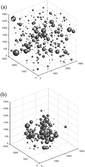
Figure 4. Typical particle distribution in EPS3 by (a) PDF and (b) Hist. method.
Download figure:
Standard image High-resolution imageA visualization of the distribution by the Hist. method is shown in figure 4(b). Using the Monte Carlo approach, 100 runs were carried out for both PDF and Hist. method to generate the resulting distribution metrics, therefore, the weighted AED, 1st NND, ASD and skewness from measured, PDF and Hist. methods are listed in table 1. According to the data in table 1, simulated weighted AEDs of particle size fulfils the measured ones. The simulated values are, however, a bit higher that may be due to the randomness of simulation and errors in the curve fitting. The distribution quantification data from the PDF method deviates further from the measured values than those derived from the Hist. method, however, the simulated particle distribution from the PDF method appears visually to be more realistic and some work in the literature should be on this basis [9, 24], which could be caused by the random generation of 1st NND data in the PDF method whereas the Hist. method attempts to conform as closely as possible to the measured data and can be further implemented into this work.
Table 1. Measured and simulated quantitative data of NPs dispersion and distribution of EPS3.
| Sample | Methods | Weighted AED (nm) | Weighted 1st NND (nm) | Weighted ASD (nm) | Skewness |
|---|---|---|---|---|---|
| EPS3 | Measured | 93.58 | 218.48 | 155.27 | 8.05 |
| 114.74 ± 16.39 | 283.89 ± 31.42 | 214.34 ± 34.19 | 5.79 ± 2.60 | ||
| Hist. | 114.74 ± 16.39 | 214.80 ± 27.57 | 149.22 ± 29.41 | 7.93 ± 2.84 |
4. Experimental results and discussion
The results of DC conductivity and space charge profiles are plotted in figures 5(a) and (b), respectively (see space charge profiles under 60% RH and saturated conditions in figure S3). It can be noticed that DC conductivities of EPS3 significantly increase after being conditioned under 60% RH but only show a little further increment in the saturated sample. A similar trend is also observed in charge injection amount from space charge profiles as listed in table 2.
Table 2. Hist. wASD, wASD (⩽10 nm) and σm of pure and EPS3 under different RH conditions.
| Sample | Values | Dry | 60% RH | Saturated |
|---|---|---|---|---|
| EPS3 | DC conductivity (S cm−1) | 4.22 ± 0.60 × 10⁻¹⁷ | 6.88 ± 0.20 × 10⁻¹⁵ | 9.87 ± 0.37 × 10⁻¹⁵ |
| Charge amount (C) | 6.64 E + 25 | 7.35 E + 25 | 9.59 × 10+25 | |
| Hist. wASD (nm) | 149.22 ± 29.41 | 127.66 ± 30.45 | 108.83 ± 31.85 | |
| wASD (⩽10, nm) | 3.00 ± 0.29 | 2.33 ± 0.27 | 0.84 ± 0.29 | |
| Pure | DC conductivity (S cm−1) | 7.32 ± 0.77 × 10⁻¹⁸ | 2.36 ± 0.23 × 10⁻¹⁶ | 2.79 ± 0.40 × 10⁻¹⁵ |
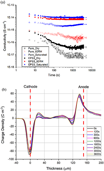
Figure 5. (a) DC conductivity curves of pure and EPS3, under different RH conditions; (b) space charge profile in the bulk of EPS3, dry.
Download figure:
Standard image High-resolution imageThe presence of moisture surely increase the charge injection and mobility: firstly, presence of water results in higher mobility of charge carriers in the matrix or percolation in part(s) of it; secondly, the formation of water shells could mitigate the inter-particle distance and traps resulting from the presence of particles, and make it easier for charge carriers to move from one trap site to another if regarding NPs as recombination centers [20, 25]. In order to better interpret the influence of water shells on charge transport, different thickness of water shells (23.7 nm for 60% RH and 53.4 nm for saturated samples which have been calculated in our previous research [18]) are introduced into the Hist. model and applied to the weighted ASD (wASD) data, as listed in table 2. It can be noticed that wASDs show a nearly linear decrement with the growth of RH. Considering the charge transport, both TAH and QMT process are highly influenced by the separation distance between adjacent NPs, herein we will relate it to the σm where wASD will be used as dTAH directly. Since the QMT would take place on a much smaller scale, if taken 10 nm as the threshold of tunneling [14], a relation between wASD (⩽10 nm) and water shell thickness can be plotted via the Hist. model in figure 6 at a step size of 2 nm from 0 to 56 nm, then different wASD of NPs which are potential for sequential tunneling processes can be calculated according to the fitting curve under various RH conditions and listed in table 2. Thus, according to equation (2), the ratio between σQMT of EPS3 under each two RH can be expressed as below in equation (7).
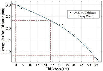
Figure 6. Weighted average surface distance (⩽10 nm) versus water shell thickness.
Download figure:
Standard image High-resolution imageThe same can be applied to σTAH as well expressed in equation (8) by assuming the same trap depth while moisture presents, where T1 = T2, N1 and N2 are the charge carrier density in bulk and can be obtained from data measured by the PEA technique by a method proposed by Liu et al [26], using equations (9) and (10), as follows:

where np(x) and nn(x) are the charge density of positive and negative charges respectively, A is the electrode area equal to 50.265 mm2 (with a radius of 4 mm), d is the thickness of samples (145 ± 10 µm), Q is the total charge amount, q= 1.602 × 10⁻¹⁹ C and N is total charge density in bulk.
Only considering the conduction caused by the presence of NPs, conductivity differences between pure and EPS3 (Δσm = σEPS3 − σ0) were calculated. As σQMT should be on the order of magnitude at 10–17 S cm−1 and σTAH is about one order of magnitude higher in dry samples [9], herein we can draw a plot to roughly exhibit how σTAH/σQMT/σEPS3/Δσm varies versus RH conditions, or in other words, different water shell thickness (see figure 7). The x-axis ratio among RH conditions is calculated by water uptakes of EPS regardless of those in the polymer matrix which has been done in our previous work [18].

Figure 7. The measured (σEPS3 and Δσm), thermally activated hopping (σTAH) and quantum mechanical tunnelling (σQMT) conductivities versus different RH conditions.
Download figure:
Standard image High-resolution image
It is obvious that the measured DC conductivity differences (Δσm) increase significantly due to the presence of moisture while σTAH and σQMT show the decrease and increase, respectively, indicating that moisture in bulk and percolation dominate the contribution to the total Δσm under 60% RH condition. The further slight increase in σEPS3 should be attributed to two reasons (under saturated condition): first, already existed and smaller growth of water uptake in the matrix should contribute to much less increment in the conductivity which could be approximately represented by the difference between σEPS3 and Δσm in figure 7; second, there is a more obvious decline of σTAH by an order of magnitude while the increase in σQMT is evident by increasing onto the order of magnitude at 10–16 S cm−1. Therefore, σQMT could play a much more significant contribution to the increment in Δσm (4.34 ± 0.97 E 16 S cm−1), indicating that QMT could be of more significance. With an increase in the RH condition, thicker water shells will lead to shorter average distances between arbitrary deep traps (which could share a similar mechanism with increase filler loadings) and charge carriers will require less energy when moving from one site to another. The resultant increased carrier mobility could lead to higher conductivity.
5. Conclusion
In conclusion, in order to explain the influence of nanoparticle distribution and water shells (moisture) on charge transport in polymer nanocomposites, a numerical estimation model has been proposed based on MDS method, TAH and QMT mechanisms. The distribution of nanoparticles/aggregates is re-virtualized by the MDS method and utilized in the estimation of charge transport in further steps. The presence of moisture could lead to significant charge injections, and for different relative humidity conditions, due to their diverse water shell thickness, the separation distances of nanoparticles where deep/shallow traps locate show an obvious reduction and consequently vary the contribution of TAH and QMT conductivities in the measured ones. The TAH mechanism plays the main role in charge transport/conduction, especially under lower RH conditions, while the QMT will be more pronounced with the growth of moisture uptake. Besides, the proposed model could be potentially extended to other research topics on electrical properties of polymer nanocomposites, such as particle size, dispersion/distribution status and filler loading concentrations which can be reflected and explained via the variation of nanoparticle surface/trap site distances. As this paper is to discuss the traps introduced by the presence of nanoparticles, their distribution will be more related to the dispersion of particles and then incorporated into charge transport behaviours. In order to get a full study on polymer nanocomposite systems, the trap distribution in the matrix will be considered and incorporated into the current model in the next step of our work.