


Abstract
In this paper, we consider a small ball placed in a liquid-filled transparent cylinder sealed at both ends. When the tube is inclined and spun about the vertical axis like a centrifuge, a heavy ball (more dense than the liquid) will accelerate to either the top or bottom end of the tube depending on its release position while a light ball (less dense than the liquid) will instead tend towards an equilibrium position in the tube. Experimental measurements of the ball's motion show large disagreements with Stokes' theory of drag force on the ball. The formation of a rotating column of liquid induced by the Coriolis force, known as a Taylor column, significantly increases the drag on the ball. In this paper, we aim to investigate the equilibrium position as well as the motion path of the ball, with a numerical solution to the 3D time-dependent Navier–Stokes equation in the rotating frame of the tube, as a function of the inclination angle and angular velocity of rotation of the tube, which are experimentally verified for a ball in a water-filled tube. Increasing both the angular velocity and inclination angle will cause the equilibrium position to shift closer to the bottom of the tube, a faster motion of the ball, and larger deflections to the side of the tube. The formation of the Taylor column was also visualised in the rotating frame with dye injection.
Export citation and abstract BibTeX RIS
1. Introduction
A centrifuge separates objects of different densities by virtue of the centrifugal force. Objects are usually flung out when swung about an axis due to the centrifugal force which points away from the axis of rotation in the rotating frame. However, that is only partly true for objects more dense than the medium they are in: for example, an iron ball in water or air. In the event where an object is less dense than its medium (e.g. a styrofoam ball in water), the object instead moves in the opposite direction and then attains a stable equilibrium position in the tube. Such counter-intuitive behaviour is reminiscent of the paradox wherein a helium ballon in a moving car jerks backwards when brakes are applied.
In this paper, we will focus our study on this perculiar behaviour exhibited by a spherical object slightly less dense than water, when it is placed in a sealed rotating tube filled with water and the tube is inclined at a variable angle. All analysis will be conducted in the rotating frame of the tube. As will be presented, oscillations about the equilibrium position are observed to be extremely overdamped, while a theory accounting for Stokes drag predicts underdamped oscillations. This mismatch in the prediction and observations of the drag force can be attributed to the formation of a Taylor column, a circulating column of fluid that an object has to drag along as it moves through a rotating body of fluid. Such a column, which is induced by the Coriolis force providing for the centripetal acceleration of moving fluid elements, increases drag on the ball due to the added inertia of the fluid column.
Experimental and theoretical studies on the motion of a solid sphere moving parallel to the axis of rotation of its fluid medium have previously revealed the effect of a Taylor column in slowing the ball [1–7]. However, analytic and empirical results obtained for these axisymmetric cases are not directly applicable to our investigation into the complex three-dimensional dynamics of the ball, which involves motion in axes both parallel and perpendicular to the tube's rotation. Hence, we instead take a more accurate approach by numerically solving the equations of motion for the ball, coupled with the Navier–Stokes equations for the fluid. Agreement with experimental measurements is obtained.
Experimental observations of the Taylor column using dye injection are also presented in following sections. Parameters such as angular frequency of rotation and inclination angle of the tube were varied to investigate their effects on the motion of the ball and fluid dynamics within the tube.
2. Static equilibrium position
Independent of the initial conditions of ball release, a light ball will always attain a stable equilibrium position in the tube which is a function of the parameters of the system, most importantly the inclination angle θ and angular velocity Ω of the tube. In this section, we will first begin with a qualitative explanation to this phenomenon followed with a quantitative analysis.
2.1. Qualitative analysis
We use the axes and variable definitions as shown in figure 1 with the origin at the base centre of the tube. In the rotating tube, the ball experiences a spatially varying acceleration field, the effective gravity, which is a vector sum of the downward gravitational acceleration and centrifugal acceleration of the tube (geff = g + ac). The equilibrium is achieved when  , i.e. no acceleration component along the tube. A light ball floats to the top surface of the tube while a a heavy ball sinks to the bottom as the normal force is required to maintain the equilibrium of forces. Rolling friction is neglected in this and subsequent analyses since it is significantly smaller in magnitude than weight and hydrodynamic forces acting on the ball as the ball used was solid with little deformations.

Figure 1. Cross-section of tube. Inclination angle is θ from vertical. Coordinates are fixed in the rotating frame of the tube.
Download figure:
Standard image High-resolution imageTo qualitatively analyse the stability of the equilibrium, we resolve the forces acting on the light and heavy balls of the same dimensions with masses m and M respectively as shown in figure 2 where the normal contact force vector N is not depicted. The effective upthrust (−ρw V geff) acting on the ball is in the opposite direction to geff, which is equivalent in magnitude to the effective weight of fluid displaced. When displaced slightly from the equilibrium, the net force points towards the equilibrium for the light ball since effective upthrust is greater than its effective weight. The reverse is true for heavy balls. An implication of this will be that when the heavy ball is released below its equilibrium point, it will fall to the bottom of the tube and when it is released above the equilibrium, it will shoot to the top of the tube. The light ball will instead tend toward the equilibrium position regardless of its point of release in the tube.

Figure 2. Force resolutions on light (left) and heavy (right) balls displaced from equilibrium. Net force on light ball is restoring while that on heavy ball is destabilising. Normal contact force is not shown for illustration purposes.
Download figure:
Standard image High-resolution imageA quick derivation accounting only for centrifugal forces will show that the oscillation frequency ω of the light ball about the equilibrium is  where ρw and ρb are the densities of water and the ball respectively. However, such oscillations are not experimentally observed due to the expectionally high damping.
2.2. Quantitative derivation
It is not immediately clear what the exact expression of the buoyant force on the ball should be, given that the ball has a finite dimension in a spatially varying effective gravitational field, since centrifugal acceleration increases with distance to the axis.
The effective gravity at each point in the rotating frame of the tube is given by
The condition for static equilibrium in the water

can then be directly integrated with respect to z to obtain pressure P.
Integrating again, this time across the surface of the ball where dS is a surface element on the ball, the expression for effective upthrust on the ball in the z-direction is obtained as follows:

Note that this reduces to the expression for the force on the CM of the ball.
With this we return to derive the expression for equilibrium position. Accounting for the finite radius of the ball and the tube and the fact that the ball is in contact with the top inner surface of the tube we write

where d is the distance from the bottom centre of the tube to the axis of rotation, illustrated in figure 1. z0 is the z coordinate of the equilibrium position of the ball, according to the axes in figure 1. The first term in the brackets in equation (4) is the result of the balance of gravitational and centrifugal accelerations along the tube, while the second and third term are obtained by considering the geometry in figure 1.
Experimental verification of equation (4) is conducted in section 5.1.
3. Dynamic motion path
In this section, we investigate the time-dependent motion of the ball released from rest from the the top of the tube with the tube rotating at a constant angular velocity. The light ball will only start moving when Ω and θ are sufficiently large. Initially the ball is deflected in the y direction due to the effect of the Coriolis force. The Coriolis force also provides for centripetal acceleration of fluid elements, causing them to form a circulating Taylor column which impedes the ball's motion, significantly damping out oscillations about the equilibrium.
Two models are presented in this section- equation of motion of the ball in the z-direction accounting for Stokes drag, as well as a numerical solution to the 3D time-dependent Navier–Stokes equation coupled with Newton's second law and torque equation on the ball. The accuracy of the models are compared in section 5.2.
3.1. Stokes drag
While the Stokes' drag is usually used in flow with low Reynolds number, it should nevertheless give a resultant drag force of around the same order of magnitude in our system. With the following expression for Stokes' drag [8, 9]:

where vb = velocity of ball and μ = dynamic viscosity of water, we write Newton's second law as such, constraining the ball to move only in the z-axis:

when the rolling condition

where μs = static coefficient of friction is satisfied. Then the motion of the light ball with amplitude A will be described by

with  and
and 
3.2. Numerical solution (Navier–Stokes)
In this section we write the governing equations for the liquid flow in the rotating frame of the tube coupled with the motion of the ball. For the fluid, we write the incompressible Navier–Stokes equation as

and the continuity equation

With that, we impose the no-slip boundary conditions on the surface of the ball:

where  angular velocity of ball and rb = position of ball in tube and on the inner surface of the tube:

where l = length of tube
With boundary conditions equations (11) and (12), we solve for u and p in equations (9) and (10). To obtain the force and torque on the ball, we first express the stress tensor as

where ![${{\bf{I}}}_{{\bf{3}}}=\left[\begin{array}{ccc}1 & 0 & 0\\ 0 & 1 & 0\\ 0 & 0 & 1\end{array}\right].$](https://content.cld.iop.org/journals/0143-0807/41/4/045806/revision2/ejpab8069ieqn6.gif)
With that we integrate for the hydrodynamic force and torque on the ball


Including the effects of the fictitious forces and torques in the rotating frame of the tube, we write the net force and torque on the ball as


where  for a homogeneous ball.
The general equations of motion for the ball are


where N = normal contact force between ball and tube,  torque from static friction to prevent slipping of ball. Equations (18) and (19) together with (9) and (10) are solved using the finite element method [10], where implicit time-stepping is implemented using the second-order backward difference formula [11]. Detailed procedures on the numerical evaluation of N and the numerical methods used are included in the appendices.
Sample plots of the velocity magnitude is shown in figure 3, which shows the Taylor column being formed and trailing the ball. Quantitative results will be discussed in section 5.2.

Figure 3. Sample velocity magnitude plot from numerical solution to section 3.2. Circular bright region denotes position of the ball. A column of fluid trailing the ball is observed.
Download figure:
Standard image High-resolution image4. Experimental set-up
An image of the experimental set-up is shown in figure 4. The tube is mounted onto a rotating platform together with a camera to capture the motion of the ball in the rotating frame.

Figure 4. Experimental set-up. The inclination of the tube is adjustable at fixed intervals. A counterweight is used to stabilise the rotation. The camera in the lab frame records the angular velocity of the tube. The camera in the rotating frame records the position of the ball.
Download figure:
Standard image High-resolution imageThe position of the ball was tracked with Tracker [12] and the parallax error due to the finite distance from the camera to the tube was accounted for.
To release the ball after the tube has spun up to a constant angular velocity, the ball was coated with a magnetic material and first held in place with an electromagnet. The electromagnet was then switched off after the tube has reached stable rotation and eddies formed during the acceleration phase have subsided.
In order to visualise the formation of the Taylor column predicted by the numerical simulation in figure 3, we allow the tube to spin up to a constant angular velocity to allow the eddies which are formed during the acceleration phase to settle before dye is injected into the fluid with a delayed dye injection system. An iron ball is robotically dragged along with a magnet placed outside the tube following the dye injection as shown in figure 5. As the iron ball is being dragged along by the magnet through the dyed region, a column of dye should follow the iron ball along in the tube as the dye is trapped in the rotating Taylor column.

Figure 5. Experimental set-sp (Taylor column visualisation). An iron ball is used instead of a light ball. After the tube has reached a constant angular velocity, dye is injected into the tube through the bottom and the iron ball is dragged through the dye region with the magnet.
Download figure:
Standard image High-resolution imageThe image of the Taylor column formed is presented in section 5.2.
5. Results and discussion
In this section, we aim to experimentally verify the accuracy of the models presented in the previous sections. Experimental data is obtained for equation (4) which governs the static equilibrium position of the ball. The dynamic motion of the ball is discussed by analysing the effects of the centrifugal and Coriolis forces and comparing the models governed by equation (6) against equations (9) and (10).
5.1. Equilibrium position
The equilibrium position z0 of the ball is plotted against Ω and θ in figures 6(a) and (b) respectively.

Figure 6. (a) Plot of z0/m against  for θ = 54.2°. An increase in Ω leads to a shift of equilibrium position closer to the bottom of the tube. z0 varies approximately with
  . (b) Plot of z0/m against θ/° for Ω = 10.3 rad s−1. An increase in θ leads to a shift of equilibrium position closer to the bottom of the tube. z0 varies approximately with
  . In both (a) and (b), between three and five experimental runs are conducted for each point. Data point plotted represents average of readings, while error bars represent standard deviation of readings.
Download figure:
Standard image High-resolution imageIncreasing either Ω or θ will cause a resultant increase in the magnitude of the centrifugal acceleration ac and the equilibrium shifts closer to the bottom of the tube to balance the component of ac and g along the tube. The x-intercept present in figure 6(b) is resultant of the finite distance from the bottom of the tube to the rotation axis in our experimental set-up (figure 4).
5.2. Dynamic motion
A ball of dimensions a = 3.5 mm is released from the top of tube of dimensions R = 18 mm, l = 0.2 m (i.e.  ). The trajectory of the ball for Ω = 9.7 rad s−1, θ = 63.2° is shown in figure 7 a plot of z against t is shown in figure 8.
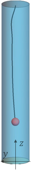
Figure 7. Trajectory of the ball from numerical simulation in section 3.2 for parameters in figure 8, Ω = 9.7 rad s−1, θ = 63.2°, a = 3.5 mm and R = 18 mm, as seen from point of view of camera in figure 4. The ball is initially deflected due to the Coriolis force to y = ymax, and eventually tends towards its equilibrium position z0.
Download figure:
Standard image High-resolution image
Figure 8. Plot of z/m against t/s for Ω = 9.7 rad s−1, θ = 63.2°, a = 3.5 mm and R = 18 mm. The large deviation between Stokes' theory and experimental observations indicate the presence of a Taylor column as a significant damping force. Error bars indicate standard deviations of raw data points used to obtain moving averages. (Elastic collision between ball and wall assumed for Stokes' drag simulation.)
Download figure:
Standard image High-resolution imageFrom figure 7, when the ball is released from the top of the tube, it is initially deflected due to the Coriolis force acting on the ball. The ball then performs small oscillations on the surface of the tube which are quickly damped out. The ball tends towards its equilibrium position as described in section 5.1.
We can clearly see from figure 8 that solely accounting for Stokes drag is insufficient to model the phenomenon accurately since a theoretical low drag on the ball will lead to the ball exceeding the equilibrium position and even shooting below the bottom of the tube. Both the wall effect and the presence of the Taylor column significantly increases drag on the ball.
The fact that the ball stays in contact with the wall increases the shear stress damping the ball's motion since no-slip condition is held at both the stationary wall surface and the moving ball surface. However, since the ball is undergoing pure rolling most of the time, this wall effect is not extremely significant. The non-laminar flow in this set-up may also explain the deviation of Stokes' law, but both these reasons do not account for the drag force being more than 2 orders of magnitude off when calculated from figure 8.
5.3. Formation of the Taylor column
Rather, it is more likely to be the formation of a Taylor column which significantly impedes the ball's motion. As illustrated in figure 9, in the rotating frame of the tube, the Coriolis force provides for centripetal acceleration of moving fluid elements, causing them to circulate in a column parallel to the tube's rotation axis. For a slow moving object in the fluid medium, this circulating column of fluid follows the object closely. The presence of this Taylor column as numerically predicted in figure 3 is verified by the experimental image in figure 10.

Figure 9. Top view of tube. As the ball moves down the tube, the fluid elements move along the streamlines. In the rotating frame, Coriolis force  acts on the fluid elements, providing for centripetal acceleration for the fluid elements to circulate near the moving ball.
Download figure:
Standard image High-resolution image
Figure 10. Taylor column experimental image. Blue dye is injected into the tube after the tube has reached constant rotation speed. The iron ball is slowly dragged through the dyed region. The image is processed to increase its contrast in grayscale, where the dark tail following the ball indicates the position of the Taylor column, which is parallel to the rotation axis Ω.
Download figure:
Standard image High-resolution imageNote that the Taylor column will only be parallel to the rotation axis in the quasistatic regime (when the ball is moving slowly). A sufficiently high velocity of the ball will cause the Taylor column to no longer be parallel to Ω, but trail the ball as shown in our numerical predictions of figure 3.
The accuracy of our numerical model can be verified by extracting a parameter which characterises the ball's motion. In the following graphs figures 11(a) and (b), vav, the average velocity of the ball in the first 1s of its motion, is plotted against Ω and θ.
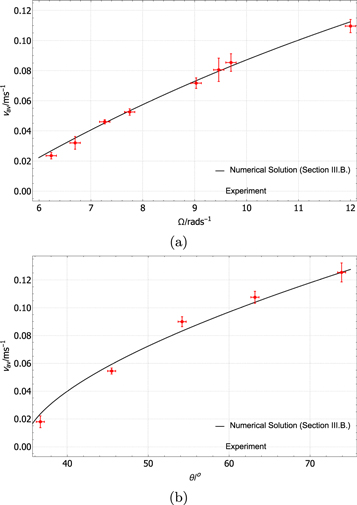
Figure 11. (a) vav/m s−1 against Ω/rad s−1(θ = 63.2°). (b) vav/m s−1 against θ/° (Ω = 12 rad s−1). Increasing either θ or Ω increases the magnitude of centrifugal force and hence the net acceleration of the ball. In both (a) and (b), between 3 and 5 experimental runs are conducted for each point. Data point plotted represents average of readings, while error bars represent standard deviation of readings.
Download figure:
Standard image High-resolution imageAs the ball initially moves down the tube with vb in the −z direction, the Coriolis force acting on the ball serves to deflect the ball to the +y-direction with  . The ball then arrives at a maximum deflection ymax before upthrust restores the ball back to the equilibrium of y = 0. The dependence of ymax on Ω and θ is shown in figures 12(a) and (b).

Figure 12. (a) ymax/m against Ω/rad s−1 (θ = 63.2°). (b) ymax/mm against θ/° (Ω = 12 rad s−1). The Coriolis force, proportional to  , results in a deflection of the ball in the +y direction. In both (a) and (b), between 3 and 5 experimental runs are conducted for each point. Data point plotted represents average of readings, while error bars represent standard deviation of readings.
Download figure:
Standard image High-resolution imageIn a rotating frame, the Coriolis force typically results in oscillations of an object. However, such oscillations are not significantly observed in our set-up due to the high damping in the system, attributed to the formation of the Taylor column.
6. Conclusion
In this paper we have analysed the statics and dynamics of a ball suspended in an inclined rotating tube filled with water. An expression for the equilibrium position, stable for a light ball and unstable for a heavy ball, has been derived in equation (4) and has been experimentally verified in figure 6.
Two models have been presented to account for the transient motion of the ball in section 3.1 as well as in section 3.2. As shown in figure 8, the model in section 3.1 underpredicts the magnitude of drag in the system. Coriolis force induces the formation of a Taylor column to account for the increased drag. The presence of the Taylor column was numerically predicted in figure 3 and verified in figure 10. A numerical solution to Navier–Stokes equations, equations (9) and (10), coupled with the equations of motion for the ball, equations (18) and (19) show improved agreement with experimental measurements.
The accuracy of the numerical drag model was verified in figure 11 and the secondary effect of the Coriolis force on the deflection of the moving ball was presented in figure 12.
Theoretical and experimental work in this paper was focused on the case of constant Ω. Our experimental observations reveal formation of clockwise water currents in the tube when the tube is undergoing angular acceleration. During this phase, the ball is dragged along by the water current and the accompanying dynamics of both the fluid and the ball may be worth further research. Other parameters such as radius a of ball and the dimensions of the tube can also be investigated.
Acknowledgments
The author of this paper would like to thank the International Young Physicist Tournament (IYPT) [13] for proposal of 'Ball in a Tube' as a competition problem, inspiring the work presented in this paper. Insightful discussions with IYPT 2017 Singapore team coaches Mr Yong Hui Lim from Massachusetts Institute of Technology, Mr Kai Yen Jee from Cornell University, Mr Joel Tan from National University of Singapore, and team leaders Mr Guan Kheng Sze from Raffles Institution and Dr Teck Seng Koh from Nanyang Technological University are greatly appreciated.
: Appendices
Appendix A.: Calculation of normal contact force
To calculate the normal contact force between the ball and the tube in equation (18), we first check for contact between the ball and the inner surface of the tube if

and

are both satisfied.
We then calculate the normal contact force

where  and check if the rolling condition is satisfied in ϕ and z directions in cylindrical coordinates, as shown in figure A1:


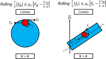
Figure A1. Rolling conditions.
Download figure:
Standard image High-resolution imageAppendix B.: Numerical solution method (BDF order 2)
Equations (9) and (10) are solved together with boundary conditions equations (11) and (12) with the second-order backward-differentiation formula (BDF2) [11] shown below:

where h is the time step dt in the transient Navier–Stokes problem.
Applying equations (24) to (9) and (10) yields the discretized equations
and

The initial conditions to equations (25) and (26) is given by

and the corresponding pressure field is solved by setting the  in equation (9) and solving with equation (27):

Appendix C.: Finite element implementation
As the time-dependent equations are converted into implicit equations for u and p, we solve these equations at each time instant with the finite element method, implemented in COMSOL Multiphysics [10, 11]. However, due to limitations in fluid–solid coupling abilities of the solver, we export the u and p fields at each time step into MATLAB, calculate the forces and torques on the ball, then calculate the new coordinate of the ball. The geometry around the ball is then remeshed at the next time step accordingly.
The element mesh for the PDE region for equations (25) and (26) is discretize with tetrahedral elements of maximum and minimum cell sizes 3.6 and 1.08 mm. Mesh refinement is conducted the region of liquid near the ball such that the maximum and minimum cell sizes take values of 1.33 mm and 0.144 mm respectively for a tube with dimensions R = 18 mm, l = 20 cm.
The forward Euler scheme is used to numerically integrate equations (18) and (19) with dt = 0.01 s.
Appendix D.: Magnetic release mechanism

Figure B1. Magnetic release mechanism. As an alternative to release using an electromagnet as described in the main sections, a mechanical release was also used. The magnetically-coated ball is initially held in place with the magnet. After the tube has reached a stable angular velocity, the motor is turned and the magnet is pulled back to release the ball.
Download figure:
Standard image High-resolution image