A Logistic Model for Counting Crowds and Flowing Particles

How many people or particles have passed there? This question is simple but significant in many physical, biological, and social situations [1–3]. Counting the total number of moving crowds or flowing particles is often a difficult task because of complexity in mobility and transport dynamics. Conceptually, this question is similar to a population dynamics that is controlled by birth and death rates or immigration and emigration [3]. In mathematical biology, the simplest population growth model is the Malthusian exponential model where the total population increases exponentially with time [4]. The logistic model is widely established in many fields for modeling and forecasting populations [5]. The logistic growth dynamics describes that the total population grows exponentially at early times and saturates to an upper limit at late times, producing a typical S-shaped curve. The upper limit represents a capacity limit in the system. In a confined space, there may be a capacity limit and thus the logistic model would be appropriate in crowd or particle counting.

In this article, the logistic model is developed to understand moving crowds or flowing particles for the total number estimation. This model sheds light on a collective contribution of crowd or particle mobility and growth rate to the total number. This model is applicable for both of static and mobile crowds and particles, probably offering a new framework for understanding transport dynamics of static or mobile crowds and particles.

First, consider a physical situation for flowing particles (conceptually, identical for moving crowds), where a fixed number of flowing particles occupy a limited number of positions in a space, as illustrated in Figure 1. As flowing particles move through a space together like flowing crowds [6–9], the total number of particles initially increases with time, reach a peak for a while, and eventually diminishes with time. In this situation, the number of particles can be modeled by a combination of particle growth and decay dynamics. This physical situation can be modeled with the factors of the first (or final) particle contribution a, the rate of growth (or decay) b, and the maximum capacity in the place c (physically, c is set by a multiple of the occupation space α and the population density β as c = αβ).

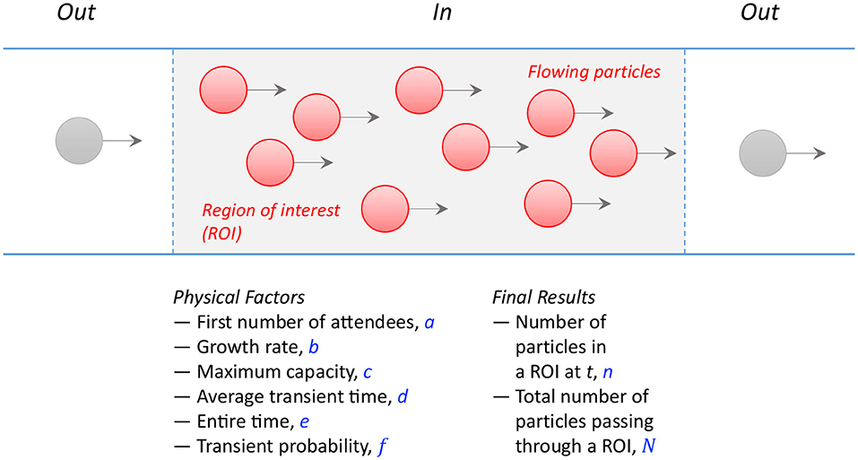
Figure 1. Illustration of a situation: when particles are flowing in a region of interest (ROI, gray) and their physical factors are given (a ~ f), an important question is how many particles (n or N) have passed through the ROI during a period.

Next, to quantify the hydrodynamic aspects of flowing particles [10, 11], the average transient time d is considered as follows. The transient time is the spent duration for particles to stay by occupying the limited positions and is responsible for the particle mobility. Assuming the entire time e for growth and decay, the transient probability f is calculated as f = d/e. By taking the transient probability, the particle mobility can be quantified.

The transient probability is useful to characterize the nature of static or mobile particles. For instance, let's think about the following two situations. In the first case, most particles may stay to pass through for a while (e.g., for 30 min) during the entire time (e.g., for 2 h), suggesting the transient probability to be $f=\frac{30}{120}=0.25$ on average. In the second case, most particles may stay for a while (e.g., for 110 min) during the entire time (e.g., for 2 h), indicating $f=\frac{110}{120}=0.92$. The first case corresponds to mobile particles (f ≪ 1.0), while the second case to static particles (f ≈ 1.0).

To describe static or mobile particles with the logistic model, the logistic growth dynamics is applied prior to a peak as [2, 4, 5]:

and after passing a peak, the logistic decay dynamics is applied as:

Here n(t) is the number of particles at a moment and is determined by the first (or final) number of particles a, the growth (or decay) rate b, the maximum capacity c, the average transient time d, the entire time e, the transient probability f = d/e, and the peak time $g=\frac{1}{2}e$. By integrating n(t) with respect to t and dividing it by the average transient time, the total number N can be estimated as:

As demonstrated in Figure 2, the logistic model is appropriate to evaluate how the particle number changes with time by the physical factors in the logistic model. In Figure 2A, for the physically feasible conditions, a = 1.0, b = 0.2, c = 100, d = 30, and e = 120 are assumed (here, time is normalized). Controlling the factors, the particle number for static or mobile particles is counted during particle growth (Equation 1) and decay dynamics (Equation 2). For simplicity, the growth dynamics is assumed to be symmetric with the decay dynamics. In Figure 2B, the contribution of the growth rate b is tested by fixing the other conditions in Figure 2A except for the variable b [a = 1.0, c = 100, d = 30, and e = 120]. Interestingly, the total number significantly increases with the growth rate b. In Figure 2C, the contribution of the transient probability f is tested by fixing the other conditions in Figure 2A except for the variable f [a = 1.0, b = 0.2, c = 100, and e = 120]. Interestingly, the total number is inversely proportional to the transient probability f (this is evident from N∝d⁻¹ and d = ef in Equation 3). The collective contribution of the growth rate and the transient probability is illustrated in Figure 2D [by fixing a = 1.0, c = 100, and e = 120], showing that the total number is significantly affected by the transient probability for most b values (b ≳ 0.2); that is, the particle mobility is crucial to determine the total number of flowing particles.

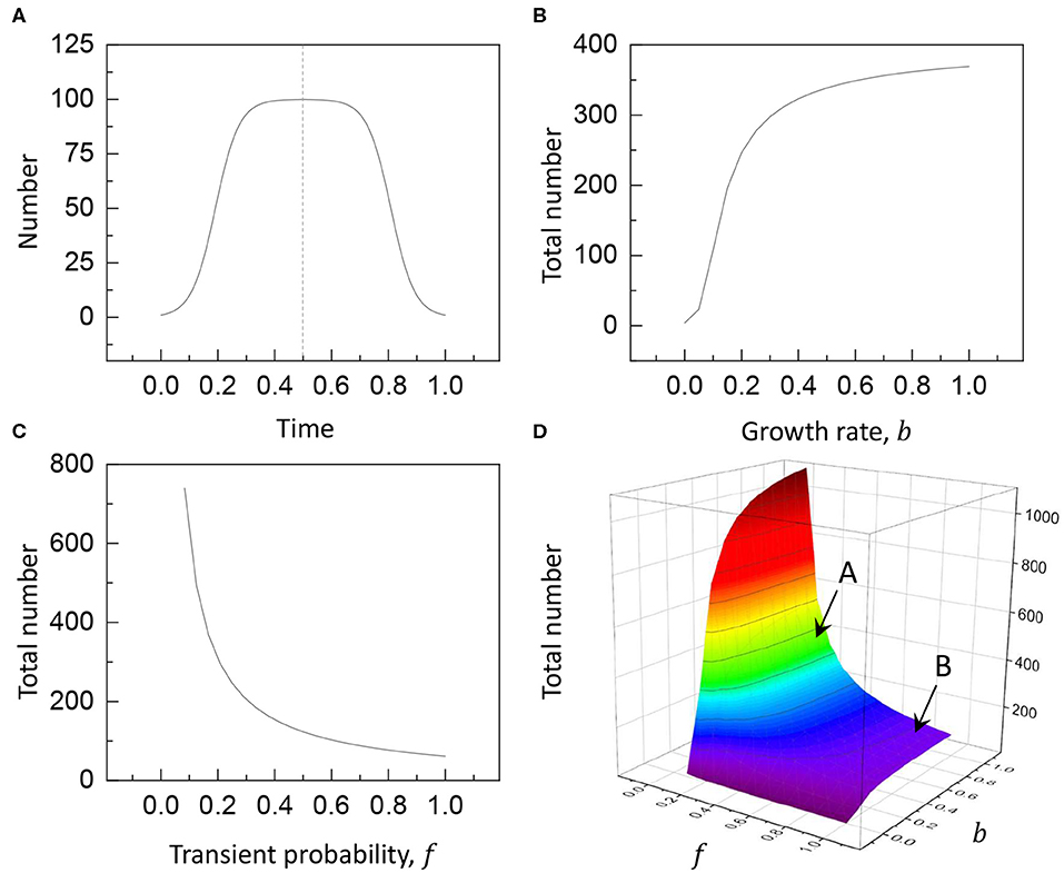
Figure 2. The logistic model: (A) the particle number n(t) changes with time [a = 1.0, b = 0.2, c = 100, d = 30, and e = 120], (B) by the contribution of the growth rate b [by fixing a = 1.0, c = 100, d = 30, and e = 120], (C) by the contribution of the transient probability f [by fixing a = 1.0, b = 0.2, c = 100, and e = 120], and (D) by the collective contribution of the growth rate b and the transient probability f [by fixing a = 1.0, c = 100, and e = 120]. Here, the total number increases by 3.7 times when the transient probability decreases to f = 0.25 (mobile particles, marked A) from f = 0.95 (static particles, marked B) for the same growth rate b = 1.0.

The logistic model is appropriate to characterize the nature of static or mobile particles. The total number of particles is illustrated in Figure 2D as a function of the transient probability and the growth rate [by fixing a = 1.0, c = 100, and e = 120]. Most interestingly, the total number is significantly affected by the transient probability, rather than the growth rate. In particular, the total number significantly increases by 3.7 times when the transient probability decreases to f = 0.25 (N = 3.7c as marked A) from f = 0.95 (N = 0.97c as marked B) for the same growth rate b = 1.0. This result clearly shows why mobile particles are more than static particles. It is noteworthy that the logistic model is applicable for both static and mobile particles by simply adjusting the physical factors. To generalize the result, the total number of particles becomes more than the maximum capacity for mobile particles (N ≫ c) and becomes less than or equal to the maximum capacity for static particles (N ≤ c).

To demonstrate the validity of the logistic model, a simulation of falling balls through a triangle grid of pegs was tested with help of the Physics Education Technology (PhET) interactive simulations (https://phet.colorado.edu) [12, 13]. In Figure 3 (see Movie S1), the number of red balls in the triangle grid increases with time at t < g and decreases with time at t > g. The measured ball number is compared with the logistic model with a = 1.0, b = 0.135, c = 38, d = 42.2, and e = 165 (N/c = 2.6), providing a good agreement between simulation and model.

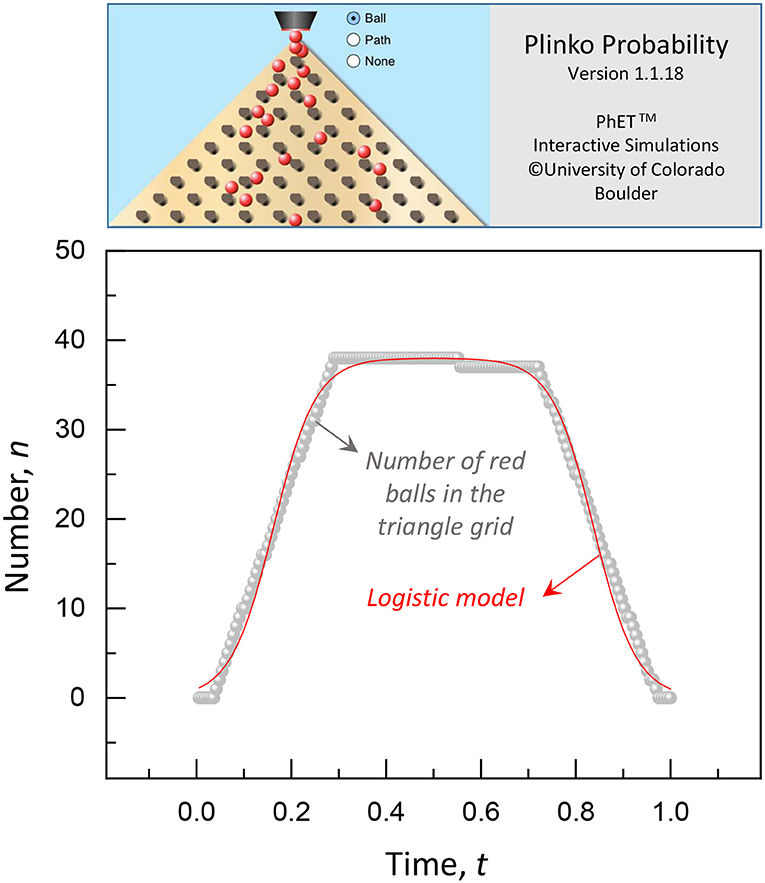
Figure 3. Simulation of falling balls through a triangle grid of pegs for the Plinko Probability by the PhET interactive simulations (Movie S1). The number of red balls in the triangle grid increases with time at t < g and decreases with time at t > g, showing a good agreement with the logistic model with a = 1.0, b = 0.135, c = 38, d = 42.2, and e = 165 (N/c = 2.6).

The logistic growth or decay dynamics is applicable to describe the number of moving crowds or flowing particles in a region of interest, based on which the total number of particles passing through the region can be estimated with a posteriori fit for the data, as demonstrated in Figure 3. Finding the parameters of the logistic dynamics is crucial for the model to work. For a priori or real-time estimation of the parameters, the early data can be analyzed and used to predict the late data. From Equation (1), the logistic differential equation is given as $\frac{dn(t)}{dt}=bn(t)(1-\frac{n(t)}{c})$ where the growth rate b and the carrying capacity c can be estimated from a priori or real-time data (the first number a can be set to be 1.0). To determine the total number N in Equation (3), the average transient time d can be obtained from a priori or real-time information and the entire time e (about twice the peak time $g=\frac{1}{2}e$) can be given or determined in real situations.

Counting the total number of particles, both a priori and a posteriori, can be applied for human crowds and planning crowd safety in places of public assembly [14–16]. In principle, human crowds are likely to stay or move in a place like flowing particles [11]. Conceptually, flowing particles are identical with moving crowds. Direct counting methods would be available with many modern technologies such as artificial intelligence, drone, and visual analysis [14, 15] to count the total number in many situations. However, direct counting would be expensive and time consuming. The approximate counting of the total number with the logistic model may be useful and applicable to estimate the particle transport through porous media in applied physics, the total number of clients visiting a store in economics [15], the crowd size of a protest in sociology [16], and the growth dynamics of bacteria in a specific colony in biology [17]. Further studies are required to verify the applicability of the logistic model in a variety of systems.

In conclusion, this study shows a theoretical frame of the logistic growth or decay dynamics that would be appropriate to estimate the total number of moving crowds or flowing particles. As demonstrated here, the model is available for both static and mobile crowds and particles. The numerical demonstration of the logistic model clearly shows how the instantaneous particle number changes with time according to the particle mobility and the growth dynamics. Practically, in physical, social, or ecological situations, the logistic model is applicable by identifying the transient probability and the growth rate to count or estimate the total number.

Data Availability Statement

The raw data supporting the conclusions of this article will be made available by the authors, without undue reservation.

Author Contributions

BW organized the research, conducted the research, analyzed the data, and wrote the manuscript.

Conflict of Interest

The author declares that the research was conducted in the absence of any commercial or financial relationships that could be construed as a potential conflict of interest.

Acknowledgments

This manuscript has been released as a pre-print at [18] (BW). This research was supported by Basic Science Research Program through the National Research Foundation of Korea (NRF) funded by the Ministry of Education (NRF-2016R1D1A1B01007133, 2019R1A6A1A03033215) and also supported by the Korea Evaluation Institute of Industrial Technology funded by the Ministry of Trade, Industry and Energy (20000423, Developing core technology of materials and processes for control of rheological properties of nanoink for printed electronics).

Supplementary Material

The Supplementary Material for this article can be found online at: https://www.frontiersin.org/articles/10.3389/fphy.2020.00212/full#supplementary-material

Movie S1. This movie shows a simulation with falling balls.

References

1. Watson R, Yip P. How many were there when it mattered? Significance. (2011) 8:104–7. doi: 10.1111/j.1740-9713.2011.00502.x
2. Jin W, McCue SW, Simpson MJ. Extended logistic growth model for heterogeneous populations. J Theor Biol. (2018) 445:51–61. doi: 10.1016/j.jtbi.2018.02.027
3. Marchetti C, Meyer PS, Ausubel JH. Human population dynamics revisited with the logistic model: how much can be modeled and predicted? Technol Forecast Soc Change. (1996) 52:1–30. doi: 10.1016/0040-1625(96)00001-7
4. Stokes M. Population ecology at work: managing game populations. Nat Educ Knowl. (2012) 3:5. Available online at: https://www.nature.com/scitable/knowledge/library/population-ecology-at-work-managing-game-populations-50937864/
5. Verhulst PF. Notice sur la loi que la population poursuit dans son accroissement. Corres Math Phys. (1838) 10:113–21.
8. Helbing D, Molnar P. Social force model for pedestrian dynamics. Phys Rev E. (1995) 51:4282–6. doi: 10.1103/PhysRevE.51.4282
9. Karamouzas I, Skinner B, Guy SJ. Universal power law governing pedestrian interactions. Phys Rev Lett. (2014) 113:238701. doi: 10.1103/PhysRevLett.113.238701
10. Bain N, Bartolo D. Dynamic response and hydrodynamics of polarized crowds. Science. (2019) 363:46–9. doi: 10.1126/science.aat9891
11. Hughes RL. The flow of human crowds. Annu Rev Fluid Mech. (2003) 35:169–82. doi: 10.1146/annurev.fluid.35.101101.161136
12. Perkins K, Adams W, Dubson M, Finkelstein N, Reid S, Wieman C, et al. PhET: interactive simulations for teaching and learning physics. Phys Teach. (2006) 44:18–23. doi: 10.1119/1.2150754
13. Wieman CE, Adams WK, Perkins KK. PhET: simulations that enhance learning. Science. (2008) 322:682–3. doi: 10.1126/science.1161948
14. Botta F, Moat HS, Preis T. Quantifying crowd size with mobile phone and Twitter data. R Soc Open Sci. (2015) 2:150162. doi: 10.1098/rsos.150162
15. Henke LL. Estimating crowd size: a multidisciplinary review and framework for analysis. Bus Stud J. (2016) 8:27–38. Available online at: https://www.abacademies.org/articles/bsjvol8number1.pdf#page=31
16. Still GK. Crowd science and crowd counting. Impact. (2019) 1:19–23. doi: 10.1080/2058802X.2019.1594138
17. Sibilo R, Perez JM, Hurth C, Pruneri V. Surface cytometer for fluorescent detection and growth monitoring of bacteria over a large field-of-view. Biomed Opt Exp. (2019) 10:2101–16. doi: 10.1364/BOE.10.002101
18. Weon BM. A logistic model for flowing particles. arXiv:1910.11995v2. (2019) Available online at: https://arxiv.org/abs/1910.11995
Keywords: flowing particles, logistic model, crowds, growth dynamics, particle mobility
Citation: Weon BM (2020) A Logistic Model for Counting Crowds and Flowing Particles. Front. Phys. 8:212. doi: 10.3389/fphy.2020.00212
Received: 06 April 2020; Accepted: 18 May 2020;
Published: 17 June 2020.
Edited by:
Wenxiang Xu, Hohai University, ChinaCopyright © 2020 Weon. This is an open-access article distributed under the terms of the Creative Commons Attribution License (CC BY). The use, distribution or reproduction in other forums is permitted, provided the original author(s) and the copyright owner(s) are credited and that the original publication in this journal is cited, in accordance with accepted academic practice. No use, distribution or reproduction is permitted which does not comply with these terms.
*Correspondence: Byung Mook Weon, bmweon@skku.edu