

Introduction
Oceans are a fundamental component of the Earth's metabolism and play a key role in global environmental and socio-economic changes. For example, oceans provide most of the life-supporting environment on the planet, host a large portion of biodiversity, play a major role in climate regulation, sustain a vibrant economy and contribute to food security worldwide (Gattuso et al., Reference Gattuso, Magnan, Bopp, Cheung, Duarte, Hinkel, McLeod E, Oschlies, Williamson, Billé, Chalastani, Gates, Irisson, Middelburg, Pörtner and Rau2018). However, ocean ecosystems are experiencing changes in physical, chemical and biological characteristics due to global warming (IPCC, 2007; Sarker et al., Reference Sarker, Feudel, Meunier, Lemke, Dutta and Wiltshire2018a, Reference Sarker, Lemke and Wiltshire2018b). Thus, it is important to understand the functioning of marine ecosystems and how they respond to climate change in order to effectively manage global marine living resources, such as fisheries (Schwerdtner Máñez et al., Reference Schwerdtner Máñez, Holm, Blight, Coll, MacDiarmid, Ojaveer, Poulsen and Tull2014).
Tropical marine ecosystems such as mangroves, seagrass, saltmarsh beds and coral reefs are rich in biodiversity, and provide both goods and services (i.e. food, employment, protection) to billions of people in Asia each year (Liquete et al., Reference Liquete, Piroddi, Macías, Druon and Zulian2016). The complex ecology of these systems is appreciated by scientists but not fully understood. The ecology of tropical marine ecosystems is driven by a variety of hydrological variables. For example, the relative importance of different factors driving the ecology of phytoplankton in shallow coastal seas depends on depth, prevailing water currents and riverine inputs to the system (Wiltshire et al., Reference Wiltshire, Boersma, Carstens, Kraberg, Peters and Scharfe2015). All of these factors are subject to temporal variations (Calijuri et al., Reference Calijuri, Dos Santos and Jati2002). Generally, light availability, temperature, salinity, pH and the concentration of macronutrients such as nitrate, phosphate and silicate are important regulators of phytoplankton biomass, productivity and community structure (Mutshinda et al., Reference Mutshinda, Troccoli-Ghinaglia, Finkel, Müller-Karger and Irwin2013b). In addition, zooplankton, the most important secondary producers in oceans, depend on phytoplankton for food and thereby also influence phytoplankton abundance through top-down control (Chassot et al., Reference Chassot, Bonhommeau, Dulvy, Mélin, Watson, Gascuel and Le Pape2010). However, understanding of how phytoplankton community dynamics are influenced by hydrological conditions remains a major challenge for ecologists (Edwards et al., Reference Edwards, Litchman and Klausmeier2013). Given the large number of biotic and abiotic parameters with simultaneous fluctuating states, it is often impossible to extricate the few key parameters driving a system.
The practical way to study the drivers of marine ecosystems is the analysis of detailed time series of taxonomic and environmental data (Irwin et al., Reference Irwin, Nelles and Finkel2012), although very few long-term datasets exist for tropical waters. In addition, efforts toward greater understanding are being constantly challenged as tropical marine systems are altered by local anthropogenic pressure (i.e. fishing, development, extraction of minerals and gas) and global climate change. This study aims to determine the drivers of tropical marine ecosystems and as a representative the Bay of Bengal (BoB) was selected. The BoB has received relatively little attention from the oceanographic community, and remained substantially under-sampled compared with the Atlantic and Pacific oceans (Hood et al., Reference Hood, Wiggert and Naqvi2013). Therefore, the biogeochemical, ecological and hydrological impacts of the BoB are not fully understood. Moreover, specific questions and hypotheses emerging from recent studies are yet to be tested. This study describes the bio-physicochemical characteristics of the BoB for better understanding of the spatial and vertical distribution of variables, and their inter- and intra-annual variability.
Materials and methods
Study area
The present study focused on the BoB, located between latitude 5° and 24°N, and longitude 79° and 100°E. The BoB is the north-eastern part of the Indian Ocean, bounded on the west and north-west by India, on the north by Bangladesh, and on the east by Myanmar and the Andaman and Nicobar Islands of India, and Sri Lanka forms the south-western boundary. As a peripheral country, the western coastline of Thailand is linked with the BoB through the Andaman Sea. The northern tip of Indonesia (i.e. Sumatra Island) forms the south-eastern boundary of the BoB. This tropical system is the largest deep-sea fan (abyssal fan) of the Earth, and governed by south-west monsoon winds from May to October and north-east monsoon winds from November to April (Schott & McCreary, Reference Schott and McCreary2001; Shankar et al., Reference Shankar, Vinayachandran and Unnikrishnan2002). This is one of the largest bays in the world and receives large flows of sediments from several rivers and water bodies from India, Bhutan, Bangladesh, Myanmar and Indonesia (Mohanty et al., Reference Mohanty, Pradhan, Nayak, Panda, Mohapatra and Mohanty2008). Due to deposition of sediments, the northern BoB has the widest shallow shelf region of the Indian Ocean (extending >185 km), which is three to four times wider off the coast of Bangladesh compared with Myanmar, the eastern coast of India and the global average of 65 km. The BoB also plays a major role in determining the climatic conditions of India and other south-east Asian countries and thus, its ecology is of paramount interest (Saraswat et al., Reference Saraswat, Manasa, Suokhrie, Saalim and Nigam2017).
Data sources and analysis
The present study is a compilation of ecological (i.e. phytoplankton, chlorophyll, primary productivity and zooplankton) and hydrological (i.e. temperature, salinity, nutrients and oxygen) datasets from the BoB. The data were obtained from World Ocean Database 2013 (WOD13) through their website (https://www.nodc.noaa.gov/OC5/SELECT/dbsearch/dbsearch.html) and Aqua MODIS via NOAA server (https://coastwatch.pfeg.noaa.gov). Phytoplankton and zooplankton data were collected from COPEPOD database (https://www.st.nmfs.noaa.gov/copepod/).
In order to obtain consistent monthly spatial data, at first we gridded the data points for each variable into a 0°5′ × 0°5′ grid. To eliminate extreme data, we calculated the mean of all data points inside the grid and eliminated those exceeding the standard deviation of that respective grid after Sarker (Reference Sarker2018). After gridding, the geospatial tabular data of different ecological and hydrological variables were interpolated using the kriging method maintaining the same geographic extent. To understand the drivers of spatial and temporal variability of ecological variables, a multivariate regression model was used for identifying the drivers of spatial variability of chlorophyll concentration in the BoB. We described the chlorophyll concentration as a linear function of both biotic (i.e. zooplankton) and abiotic (i.e. temperature, salinity, dissolved oxygen, silicate, nitrate and phosphate) variables. Letting N i and X j,i denote the chlorophyll concentration at location i and the value of j th explanatory variable at location i, respectively. The model equation is:
 $$N_i = \alpha + \sum\limits_{\,j = 1}^n {\beta _jX_{\,j\comma i} + \varepsilon } $$
Where α is intercept, β j is the effect of the j thexplanatory variable on the chlorophyll concentration and ε is the residual term.
To understand the long-term trend in sea surface temperature (SST) and surface chlorophyll concentration, we performed linear regression of long-term data on SST and chlorophyll with respect to time. Similarly, to understand the long-term trend in vertical profile, we performed linear regression of vertical data on temperature, salinity, nutrients and dissolved oxygen with respect to time.
In general, the length of time series for each variable differs depending on the dataset of the sampling period. For the spatial variability of bio-physicochemical variables, we used annual mean data from 1997 to 2018. To understand the vertical variability of bio-physicochemical variables, we used data from March to April of the years 1976, 1995, 2007 and 2016. SST data from 1950 to 2018, and primary productivity data from 1997 to 2018 were used for long-term trend analysis. To analyse the long-term trend in vertical distribution of bio-physicochemical variables, data from March to April of the years 1978, 1988, 1995, 2007 and 2016 were used. As we considered different datasets for different analyses (i.e. mean data for spatial variability, same season data for long-term trend in vertical profiles and annual mean data for long-term trend analysis), they do not have an impact on the sensitivity of the results.
Results and discussion
The primary goal of this study is to provide an overview of bio-physicochemical characteristics of the BoB. Spatial and temporal (i.e. seasonal and long-term) variability in bio-physicochemical parameters (i.e. SST, salinity, dissolved oxygen, nutrients and chlorophyll) of the BoB are discussed along with the ecological features as a function of hydrological variables.
Variability in bio-physicochemical parameters: BoB vs Arabian Sea (AS)
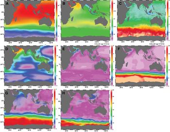
The annual mean SST in the BoB was relatively higher than the AS, i.e. 28.80°C vs 27.13°C. SST in the BoB is greatly influenced by the presence of land masses on its three sides (Shamsad et al., Reference Shamsad, Farukh, Chowdhury and Basak2012) and typical water temperature ranged between 25–30°C. High SST in the BoB is related to stratification, which is comparatively higher than the AS due to the large amount of river discharge and precipitation (Da Silva et al., Reference Da Silva, Mazumder, Mapder, Peketi, Joshi, Shaji, Mahalakshmi, Sawant, Naik, Carvalho and Molletti2017; Li et al., Reference Li, Han, Wang, Ravichandran, Lee and Shinoda2017). Mixing processes in the AS were higher due to persistent strong winds coming from the mountains of east Africa, while the winds over the BoB are sluggish in nature (Fine et al., Reference Fine, Smethie, Bullister, Rhein, Min, Warner, Poisson and Weiss2008). Because of less mixing over the surface of the BoB, the level of SST over the AS is always lower than the BoB. A strong gradient in SST was observed in the BoB, from the coast to the open sea (Figure 1). SST distribution revealed a minimum temperature in the north-east Bay and a maximum in the south Andaman. The northern BoB close to Bangladesh is generally cooler than the southern BoB. In the central Bay (88°E), SST was 29°C between 9°N and 15°N that reduced to 28.5°C by 20°N.

Fig. 1. Spatial variability in monthly mean condition of bio-physicochemical variables in the Indian Ocean. (A) Sea surface temperature (°C), (B) salinity, (C) dissolved oxygen (ml l−1), (D) zooplankton biomass (mg C m−3), (E) chlorophyll concentration (mg m−3), (F) nitrate (μmol l−1), (G) phosphate (μmol l−1) and (H) silicate (μmol l−1).
The spatial distribution of sea surface salinity was higher in the AS than the BoB (Figure 1), i.e. 35.16 vs 33.05, although both basins share the same latitude band and are affected by the semi-annually reversing monsoonal winds (D'Addezio et al., Reference D'Addezio, Subrahmanyam, Nyadjro and Murty2015). The elevated level of salinity in the AS is due to higher evaporation and lower precipitation regimes, and also attributed to the influence of high saline waters from the Red Sea and Persian Gulf (Rao & Sivakumar, Reference Rao and Sivakumar2003). In contrast, the BoB receives much higher precipitation, which typically overwhelms evaporation and also large amounts of freshwater run-off from the Ganges-Brahmaputra-Meghna rivers system (Sengupta et al., Reference Sengupta, Bharath Raj and Shenoi2006). Sea surface salinity in the central Bay was 33.5 between 9°N and 15°N and decreased to 28 at 20°N. The salinity gradient in the upper 50 m was ~0.02 m−1 at 9°N, while it was ~0.14 m−1 at 20°N, indicating a strong signal of freshwater influx in the northern part of the BoB. In the western Bay, the level of salinity was 34 at 12°N and decreased northwards to 24 at 19°N. The salinity gradient in the upper 50 m was stronger, i.e. 0.2 m−1 at 19°N and 85°E. The lowest salinity was observed in the eastern part belonging to the area characterized by higher SST. Such a low salinity tongue can be attributed to wind-driven coastal currents leading to an offshore Ekman transport that pushes the southward migrating low salinity plume away from the coast (Shetye, Reference Shetye1993).
In the BoB, a strong gradient in dissolved oxygen concentration was observed with low levels near the coast and high levels in the open sea (Figure 1). Average surface oxygen concentration in the BoB was ~4 ml l−1, classified as the oxygen minimum zone (OMZ). This is because the ventilation age in both the AS and the BoB is 30 years or longer due to their closed northern boundaries (Fine et al., Reference Fine, Smethie, Bullister, Rhein, Min, Warner, Poisson and Weiss2008). Though the OMZ in the BoB is strong, it is rather weaker than the OMZ in the AS. The primary source of oxygen for both the AS and the BoB originates from the southern hemisphere (Figure 1). Highly oxygenated, intermediate water is formed along the northern edge of the Antarctic Circumpolar Current, and subsequently spreads throughout the Indian Ocean. In the AS, other sources of oxygenated water include the Persian Gulf water (PGW) and Red Sea water (RSW), with PGW entering the AS just beneath the thermocline (Bower et al., Reference Bower, Hunt and Price2000) and RSW at intermediate depths, 300–1000 m (Beal et al., Reference Beal, Ffield and Gordon2000; Bower et al., Reference Bower, Johns, Fratantoni and Peters2005). In addition, water from the Indonesian Throughflow (ITF) influences the upper Indian Ocean, including properties of thermocline waters in the AS (Haines et al., Reference Haines, Fine, Luther and Ji1999; Song et al., Reference Song, Gordon and Visbeck2004). Mixing by mesoscale eddies can also spread oxygen (and other biological variables) in both sub-basins. The occurrence of an OMZ was noticed at depth below 100 m in the BoB (north of the equator) and the boundary of the OMZ followed the depth of thermocline. The OMZ was widespread throughout the subsurface depths (100–1500 m) in the BoB and oxygen levels increased to the south of the equator (McCreary et al., Reference McCreary, Yu, Hood, Vinaychandran, Furue, Ishida and Richards2013).
The spatial distribution of nutrients (silicate, nitrate and phosphate) showed that coastal areas are rich in nutrients, but their concentrations are low in open seas (Figure 1). This could be related to freshwater influx and residual flow from the surrounding rivers in the northern BoB. Lower levels of silicate (<2 μmol l−1), which is typical in the open ocean, was common in the southern BoB. The major source of nutrients in the BoB is the discharge of surrounding river systems. For example, the Ganges, Godavari and Irrawaddy rivers account for ~75–80% of the total river transport of nitrogen (N) and phosphorus (P) to the coastal waters of BoB (Pedde et al., Reference Pedde, Kroeze, Mayorga and Seitzinger2017). Rivers draining into the western BoB generally contain higher N and P export compared with the rivers of the eastern BoB. The dominant sources of different forms of N and P differ across the basins, although anthropogenic activities contribute higher levels of N and P in the western BoB. In addition, Broecker et al. (Reference Broecker, Toggweiler and Takahashi1980) found that BoB Fan sediment serves as a major source of nutrient elements.
The zooplankton concentration is less in the BoB compared with the AS. A strong gradient of high to low zooplankton biomass was observed in the BoB, from the coast to the offshore area (Figure 1). In the central Bay, zooplankton carbon biomass is <5 mg C m−3, while it is much higher in the coastal area (>10 mg C m−3). The average biomass in the coastal area and southern Bay were twice that of the central Bay due to the frequent swarms and higher bio-volumes of pyrosomes (i.e. free-floating tunicates) in the former (Fernandes & Ramaiah, Reference Fernandes and Ramaiah2008).
The BoB is traditionally considered to be a region of lesser biological productivity and this study also corroborates that fact. The surface chlorophyll-a in the central BoB weakly increased from 0.06 mg m−3 in the south to 0.28 mg m−3 in the north (Figure 1). In the AS, the variation ranged from 0.32–1.12 mg m−3, indicating 4–5 times higher chlorophyll-a concentration than the BoB. The monsoon rainfall and freshwater discharge from rivers freshen the upper layers of the BoB and during this time SST was warmer by 1.5–2°C than in the central AS (Prasanna Kumar et al., Reference Prasanna Kumar, Muraleedharan, Prasad, Gauns, Ramaiah, de Souza, Sardesai and Madhupratap2002). This leads to a strongly stratified surface layer in the BoB. In addition, the weaker winds over the Bay are unable to erode that stratified surface layer, thereby restricting the turbulent wind-driven vertical mixing to a shallow depth of <20 m (Mahadevan et al., Reference Mahadevan, Paluszkiewicz, Ravichandran, Sengupta and Tandon2016). This inhibits introduction of nutrients from below, close to the mixed layer bottom, into the upper layers. Advection of nutrient-rich water into the euphotic zone makes the AS highly productive and this process is unlikely in the BoB.
In order to understand which parameters drive the spatial variability in chlorophyll, we analysed chlorophyll concentration data in relation to biotic (i.e. zooplankton) and abiotic (i.e. temperature, salinity, dissolved oxygen, silicate, nitrate and phosphate) variables. The multivariate regression analysis showed that seven explanatory variables jointly explain 81% chlorophyll variability in the BoB. SST was the best predictor of spatial variability in chlorophyll a concentration and explained 27% variation in primary production. Phosphate, nitrate and silicate concentrations were also important predictors of primary productivity in the BoB that explained 22, 10 and 8% of the variation, respectively. Zooplankton biomass was another important predictor of chlorophyll a distribution (i.e. explained 10% variation), while salinity and dissolved oxygen explained 3% and 2% chlorophyll variability in the BoB. Chlorophyll a had a significant negative correlation with temperature (P < 0.001) and zooplankton (P < 0.05). In addition, there was a significant positive correlation between chlorophyll and silicate (P < 0.05), nitrate (P < 0.05), phosphate (P < 0.001), dissolved oxygen (P < 0.05) and salinity (P < 0.05). The variability in phytoplankton assemblages and their dynamics are the outcome of a complex interplay between biotic and abiotic factors (Mutshinda et al., Reference Mutshinda, Troccoli-Ghinaglia, Finkel, Müller-Karger and Irwin2013b, Reference Mutshinda, Finkel, Widdicombe and Irwin2016; Jamil et al., Reference Jamil, Kruk and ter Braak2014). For example, Recknagel et al. (Reference Recknagel, French, Harkonen and Yabunaka1997) and Kim et al. (Reference Kim, Jeong, Whigham and Joo2007) found micronutrients (i.e. silicate, nitrate and phosphate) are important to correctly predict the variability of phytoplankton abundance. In addition, temperature and salinity are also found to regulate phytoplankton biomass, productivity and community structure (Mutshinda et al., Reference Mutshinda, Finkel and Irwin2013a). The grazing pressure of zooplankton also limits the growth of phytoplankton (Huber & Gaedke, Reference Huber and Gaedke2006). These facts are in line with our findings.
Vertical bio-physicochemical variability in the BoB
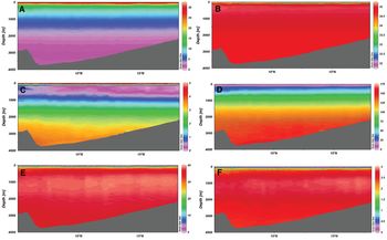
Vertical distributions of temperature, salinity, silicate, nitrate, phosphate and dissolved oxygen concentration in the BoB at 20°S are shown in Figure 2. Up to 500 m depth, all these variables exhibited strong vertical gradients. As for vertical chlorophyll profile, there was a maximum concentration of chlorophyll below the surface water (Figure 2), which is known as deep chlorophyll maximum (DCM) (Anderson, Reference Anderson1969; Jochem et al., Reference Jochem, Pollehne and Zeitzschel1993). A typical vertical profile of temperature, salinity, nutrients and dissolved oxygen focusing DCM along with the vertical distribution of phytoplankton is shown in Figure 3. A DCM was found at the depth range 45–55 m in the coastal region and at depths 55–100 m in the open sea. This is further supported by the highest occurrence of subsurface biogenic silica (diatoms) in the BoB, as observed by Gupta & Sarma (Reference Gupta and Sarma1997).

Fig. 2. Vertical variation of (A) temperature, (B) salinity, (C) dissolved oxygen, (D) silicate, (E) nitrate and (F) phosphate in the Bay of Bengal.

Fig. 3. Vertical profiles of bio-physicochemical variables focusing on the deep chlorophyll maximum (DCM) in the Bay of Bengal.
The DCM was located underneath the surface mixed layer, in the oxycline and nutricline zones, and above the seasonal thermocline/pycnocline. The subsurface maximum of chlorophyll was within the depth range of the nitracline, which is a sharp transition between the nutrient-free mixed layer and the nutrient-rich deep regime. Thus, the subsurface chlorophyll maximum appears to develop after exhaustion of surface nitrate, while the growth of plankters is merely limited within and below the nitracline (Sarma & Aswanikumar, Reference Sarma and Aswanikumar1991). The nitracline and chlorophyll maxima stay with the seasonal thermocline (Fasham et al., Reference Fasham, Platt, Irwin and Jones1985). The mechanisms involved in the formation and maintenance of the DCM include higher in-situ growth at the nutricline than in the upper mixed layer, physiological acclimation to low irradiance and high nutrient concentrations, accumulation of sinking phytoplankton at density gradients, behavioural aggregation of phytoplankton groups, and differential grazing on phytoplankton (Cullen, Reference Cullen1982; Pérez et al., Reference Pérez, Fernández, Marañón, Morán and Zubkov2006).
The distribution of phytoplankton indicates diatoms as the dominant group in the DCM (Figure 4). Species of Bacteriastrum comosum, Cerataulina pelagica, Chaetoceros affinis, Chaetoceros, Coscinodiscus, Dactyliosolen, Navicula, Nitzschia closterium and N. delicatissima showed peak abundance at DCM. The chlorophyll concentration changed substantially with increasing depth, with a surface value of ~0.10 μg l−1 that increased to a maximum of >0.45 μg l−1 at the DCM and then decreased to <0.02 μg l−1 at a depth of 150 m. The magnitude of the chlorophyll maximum at the DCM layer is ~5 times higher than the level at the surface. The depth-integrated chlorophyll concentration up to 150 m ranged between 1.00–1.50 μg l−1.

Fig. 4. Vertical profiles of phytoplankton distributions focusing on the deep chlorophyll maximum (DCM) in the Bay of Bengal.
There was a positive relationship (r = 0.84, P < 0.001) between the MLD (mixed layer depth) and the DCM (Figure 5), suggesting that the DCM increases with the increase of the MLD. The MLD represents the influence of turbulent wind mixing and the nature of vertical thermal diffusion. The mixed layer depth is an important predictor of the DCM which corresponds to a change in the MLD, the thickness and depth of the DCM therefore would be changed greatly (Coon et al., Reference Coon, Lopez, Richerson, Powell and Goldman1987; Murty et al., Reference Murty, Gupta, Sarma, Rao, Jyothi, Shastri and Supraveena2000). The factors (i.e. wind stress curl, associated Ekman pumping and heat flux at the sea surface) that are affecting the surface mixed layer, seasonal thermocline and hence the meso-scale circulation could also influence the DCM in the BoB (Murty et al., Reference Murty, Gupta, Sarma, Rao, Jyothi, Shastri and Supraveena2000). A positive relationship was also observed between the DCM and the depth of the stability maximum (Figure 5; r = 0.89, P < 0.001). This finding is consistent with previous studies in the tropical Indian Ocean (Brock et al., Reference Brock, Sathyendranath and Platt1993) and in the subtropical Azores front (Fasham et al., Reference Fasham, Platt, Irwin and Jones1985).Thermocline depth and DCM were positively related (Figure 5; r = 0.91, P < 0.001), while a significant negative relationship was observed between the chlorophyll maximum and the depth of the DCM (Figure 5; r = −0.82, P < 0.001). According to Murty et al. (Reference Murty, Gupta, Sarma, Rao, Jyothi, Shastri and Supraveena2000), chlorophyll a concentration was higher when the DCM was associated with the thermocline. This means surface stratification due to the halocline has no influence on the DCM, but there is an influence of vertical thermal diffusion on the DCM. This is in line with the coupled model study of Varela et al. (Reference Varela, Cruzado, Tintoré and García-Ladona1992). A significant correlation was noted between the depth of subsurface chlorophyll maxima and the depth of the nitrocline (Figure 6; r = 0.83; P < 0.001). This suggests that regenerated nutrients may exert an important influence on the subsurface chlorophyll maxima (Sarma & Aswanikumar, Reference Sarma and Aswanikumar1991).

Fig. 5. Relationship of deep chlorophyll maximum (DCM) with chlorophyll maximum (CMAX), mixed layer depth (MLD), depth of stability maximum (DSM) and thermocline depth.

Fig. 6. Relationship of deep chlorophyll maximum (DCM) to nitracline depth in the Bay of Bengal.
Seasonal bio-physicochemical variability in the BoB
The intra-annual course (seasonal cycle) of all selected variables for the BoB, including the inherent variability, are shown in Figure 7. Maximum silicate concentration was 9.67 μmol l−1 in August and the level was at a minimum 1.86 μmol l−1 in December. The concentrations of nitrate and phosphate were maximum in July and minimum in February and April, respectively. The seasonal distribution of temperature was bi-modal in the BoB, with the primary peak during May to June and a secondary peak in October. Mean annual temperature was 28.49°C, and maximum salinity was 29.2 in February and a minimum of 9.1 during July. Maximum rainfall occurred during May to August, while the rainfall was lower in winter months. Using a time lag of one month for the high rainfall and freshening of seawater, a significantly (R 2 = 0.53 at P < 0.01) negative relationship between rainfall and salinity was noted. The salinity was decreased after March due to input from riverine sources. The occurrence of higher salinity (weekly mean concentration >28.5) in the BoB was mostly restricted in the months of December to March. Transport from the north direction into the BoB was lower during October to April and the salinity shifts were related to run-off rates of the river systems. Although the run-offs of rivers were largely a proxy for freshwater influence in the BoB, it does indicate that increased run-off is likely to dominate the system during April to late September and decrease the salinity. Moreover, the drop in temperature after May was related to high rainfall events over the BoB. The biomass of phytoplankton and zooplankton was at a maximum during October and January, and a minimum during June and October.

Fig. 7. Seasonal variability in bio-physicochemical parameters in the Bay of Bengal.
So, how do different biotic and abiotic variables control the seasonal dynamics of phytoplankton in the BoB? Phytoplankton abundance, as the main food source, governs the abundance of herbivorous zooplankton, which in turn regulates the level of planktivorous organisms (Sarker & Wiltshire, Reference Sarker and Wiltshire2017). In the oceanic ecosystem, phytoplankton dynamics are regulated by both ‘bottom-up’ factors (e.g. light, temperature and nutrients) and ‘top down’ mechanisms (e.g. zooplankton grazing) (Wiltshire et al., Reference Wiltshire, Boersma, Carstens, Kraberg, Peters and Scharfe2015).We found that higher temperatures are responsible for lower growth rates in phytoplankton and zooplankton. In addition, low nutrient conditions result in low growth rates and conversely, high nutrient conditions result in high algal growth rates. Analysis of the monthly data showed that there was a time lag of up to one month between the phytoplankton and silicate peak during the south-west monsoon. The abundance of phytoplankton increases in response to increased silicate concentration. How early and how steep the abundance curves were during this period depended on the availability of nutrients. Silicate and phosphate were found to decline by the end of May, whereas the level of nitrate declined more slowly, at the end of August. This is evidence of timing differences for uptake of nutrients, for example, phosphate and silicate decrease most rapidly. Due to uptake by phytoplankton, nutrients remain at low levels during September to April. By then, the level of phytoplankton (diatoms) increased in biomass to their typical winter concentrations. Copepods and larval fish are the dominant grazers of phytoplankton (Nair et al., Reference Nair, Nair, Achuthankutty and Madhupratap1981; Baliarsingh et al., Reference Baliarsingh, Srichandan, Lotliker, Kumar and Sahu2018), especially from May to September. In the months of March to August, phytoplankton growth is limited due to zooplankton grazing. During this time zooplankton densities were higher and high grazing leads to lower numbers of phytoplankton (Mieruch et al., Reference Mieruch, Freund, Feudel, Boersma, Janisch and Wiltshire2010). At the end of August, zooplankton tend to decrease in density and phytoplankton start to grow. This results in higher phytoplankton abundance in late August and as phytoplankton start to grow, nutrients start to decrease rapidly from August onwards.
We highlight the importance of temperature, nutrients, zooplankton, and to a lesser extent salinity and rainfall, in the abundance of phytoplankton in the BoB on an annual basis. High zooplankton abundances were associated with high phytoplankton abundances. Nutrient patterns were found to be governed by the growth patterns of phytoplankton. The rate at which nutrients were used up by phytoplankton, particularly in stoichiometric terms, indicates the relative requirement of different nutrients by phytoplankton. When phytoplankton abundance started to increase, nutrients such as phosphate, nitrate and silicate are taken up at a greater rate.
Long-term trend of bio-physicochemical variables in the BoB
The time series data of different environmental variables in the BoB with respect to inter-annual variability is shown in Figure 8. A significant positive trend in temperature was observed in the BoB. Temperature is one of the fundamental factors governing the oceanic water masses and a key indicator of climate change (Roemmich et al., Reference Roemmich, John Gould and Gilson2012). About 90% of the excess heat added to the Earth's climate system has been stored in the oceans since the 1960s (Levitus et al., Reference Levitus, Antonov, Wang, Delworth, Dixon and Broccoli2001). Studies found that the entire Indian Ocean has been warming over the past half-century (Chambers et al., Reference Chambers, Tapley and Stewart1999; Alory et al., Reference Alory, Wijffels and Meyers2007; Du & Xie, Reference Du and Xie2008; Rao et al., Reference Rao, Dhakate, Saha, Mahapatra, Chaudhari, Pokhrel and Sahu2012; Dong et al., Reference Dong, Zhou and Wu2014). A significant increase of water temperature in the BoB, as noted in this study, is supported by the findings of D'Mello & Prasanna Kumar (Reference D'Mello and Prasanna Kumar2016), who claimed an increase in SST at a rate of 0.014°C per year over the period of 1960–2011. Adding to that, the sunspot cycle was partially controlling the rising trend of temperature in the BoB (White et al., Reference White, Lean, Cayan and Dettinger1997). Moreover, the ocean-atmospheric coupling climatic mode, likewise the negative phase of Indian Ocean Dipole, which results in comparatively higher SST in the eastern Indian ocean could also be responsible for temperature rise in the basin (Ng et al., Reference Ng, Cai and Walsh2014). We found a significant linear increase of temperature at the rate of 0.01°C year−1 in the BoB, but there was a significant decreasing trend in primary productivity in that area. The spatial distribution of chlorophyll computed from the observations and historical simulations indicate a decreasing trend in the western Indian Ocean (Roxy et al., Reference Roxy, Modi, Murtugudde, Valsala, Panickal, Ravichandran, Vichi and Lévy2016). This negative trend in primary productivity is in line with a global decrease in primary productivity (Boyce et al., Reference Boyce, Lewis and Worm2010; Gregg & Rousseaux, Reference Gregg and Rousseaux2014) and related to the warming trend in the BoB (Roxy et al., Reference Roxy, Modi, Murtugudde, Valsala, Panickal, Ravichandran, Vichi and Lévy2016). The warming will unquestionably influence marine plankton as it directly impacts both the availability of growth-limiting resources and the ecological processes governing the biomass distributions and annual cycles (Behrenfeld, Reference Behrenfeld2014). Apart from temperature, light, nutrients and grazing of zooplankton, diseases due to infectious microorganisms may also play a role in the declining primary productivity (Behrenfeld, Reference Behrenfeld2014; Sarker & Wiltshire, Reference Sarker and Wiltshire2017; Sarker et al., Reference Sarker, Lemke and Wiltshire2018b). However, due to the lack of continuous data for these variables their long-term causal relationship with primary productivity was beyond the scope of this study.

Fig. 8. Long-term trend in SST (A) and primary productivity (B) in the Bay of Bengal.
The vertical structure of different environmental variables in the BoB also showed a change over the long-term period (Figure 9). A linear regression analysis yielded a significant positive trend for temperature (P < 0.01) and nitrate (P < 0.01), and a significant negative trend for salinity (P < 0.001), oxygen (P < 0.01), silicate (P < 0.001) and phosphate (P < 0.01). We found a significant increase of temperature at the rate of 0.4°C per decade. In contrast, a significantly negative trend of salinity (0.6 per decade) was recorded. Oxygen also showed a significantly negative trend, 0.67 ml l−1 per decade. The declining trend of oxygen indicates the possibility of hypoxia in the BoB in the long term (Matear & Hirst, Reference Matear and Hirst2003; Sturdivant et al., Reference Sturdivant, Seitz and Diaz2013). Silicate, nitrate and phosphate also showed a significantly decreasing trend. The correlation coefficient between nitrate and phosphate is 0.81, suggesting that nitrate and phosphate varied together with a mean molar ratio of 16:1. The salinity distribution in the BoB was mostly governed by the amount of freshwater run-off from the rivers (Sengupta et al., Reference Sengupta, Bharath Raj and Shenoi2006), the precipitation linked to the monsoon that is still unpredictable as well as the entrance of high saline water from the AS during the summer. There was a linearly decreasing trend in surface salinity over the last 50-year period in the northern BoB (Aretxabaleta et al., Reference Aretxabaleta, Smith and Ballabrera-Poy2015). The salinity of the BoB is mostly influenced by the amount of freshwater input and precipitation. In addition, the increased atmospheric temperature might have caused a higher melting rate of Himalayan ice that also decreased the salinity in the mouth of the Ganges river system (Mitra et al., Reference Mitra, Banerjee, Sengupta and Gangopadhyay2009). Thus, the hydrological cycle (i.e. rainfall and evaporation) and the freshwater discharge would be the correct explanation of the decreasing ascending pattern. Trends in the concentration of dissolved oxygen in the BoB over the last several decades remained consistent according to the findings of Joos et al. (Reference Joos, Plattner, Stocker, Körtzinger and Wallace2003). The positive trend in nitrate might be related to an increase in remineralization as a consequence of the OMZ development in relation to long-term decrease in oxygen. Moreover, atmospheric nitrogen might be an additional source of N. Human activities contribute substantially to the reactive N load in the atmosphere over the continents (Duce et al., Reference Duce, LaRoche, Altieri, Arrigo, Baker, Capone, Cornell, Dentener, Galloway, Ganeshram, Geider, Jickells, Kuypers, Langlois, Liss, Liu, Middelburg, Moore, Nickovic, Oschlies, Pedersen, Prospero, Schlitzer, Seitzinger, Sorensen, Uematsu, Ulloa, Voss, Ward and Zamora2008). Global models estimate that the anthropogenic component of atmospheric N deposition into the ocean accounts for up to one third of the ocean's external N supply (Altieri et al., Reference Altieri, Fawcett, Peters, Sigman and Hastings2016). In addition, diatoms such as Rhizosolenia can contribute N from the deep waters to the euphotic zone by means of vertical migration and thereby contribute to the fresh supply of N in the ecosystem (Singler & Villareal, Reference Singler and Villareal2005). It is evident that the phytoplankton community in the BoB is dominated by diatoms (Sampathkumar et al., Reference Sampathkumar, Balakrishnan, Kamalakannan, Sankar, Ramkumar, Ramesh, Kabilan, Sureshkumar, Thenmozhi, Gopinath, Jayasudha, Arokiyasundram, Lenin and Balasubramanian2015; Biswas et al., Reference Biswas, Shaik, Bandyopadhyay and Chowdhury2017). Thus, reduction of silicate and phosphate might be the result of an abundance of diatoms, which require silicate and phosphate for their growth. The declining trend of silicate and phosphate may also be related to elevated levels of nutrients discharging from the river systems into the BoB (Pedde et al., Reference Pedde, Kroeze, Mayorga and Seitzinger2017).

Fig. 9. Long-term trend in vertical profile of bio-physicochemical variable in the Bay of Bengal.
Conclusion
This study described the bio-physicochemical characteristics of the BoB and the results have wider implications for understanding the ecology of tropical seas. First, we showed the spatial variation in the bio-physicochemical parameters of the BoB along with the drivers of spatial variability of ecology, i.e. chlorophyll. Second, the vertical profile of bio-physicochemical parameters was analysed. To elucidate the vertical profile, we explained the DCM, which is a typical feature in the tropical marine ecosystem. Third, we showed both inter-annual and intra-annual variation of bio-physicochemical parameters. This study thus identified the important explanatory variables associated with the changes in spatial and temporal characteristics of bio-physicochemical parameters in the BoB. The findings indicate that changes in biotic and abiotic factors are expected to have a consequence on the abundance of phytoplankton, which might ultimately affect the higher trophic levels, for example fish, and be useful to elucidate the ecology of tropical seas under climate change scenarios.
Acknowledgements
The authors are grateful to the reviewers for their comments and suggestions to improve the manuscript at this stage. We also thank associate editor of JMBA, David Paterson for updating the language of the manuscript.