A Review of H2, CH4, and Hydrocarbon Formation in Experimental Serpentinization Using Network Analysis
 Samuel Barbier1,2†
  Fang Huang3,4*†
  Muriel Andreani1
  Renbiao Tao1
  Jihua Hao1
  Ahmed Eleish3
  Anirudh Prabhu3
  Osama Minhas3
  Kathleen Fontaine3
  Peter Fox3
  Isabelle Daniel1
- 1Univ Lyon, Univ Lyon 1, ENSL, CNRS, Laboratoire de Géologie de Lyon UMR 5276, Villeurbanne, France
- 2Total CSTJF, Pau, France
- 3Tetherless World Constellation, Rensselaer Polytechnic Institute, Troy, NY, United States
- 4CSIRO Mineral Resources, Kensington, WA, Australia
The origin of methane and light hydrocarbons (HCs) in natural fluids from serpentinization has commonly been attributed to the abiotic reduction of oxidized carbon by H2 through Fischer-Tropsch-type (FTT) reactions. Multiple experimental serpentinization studies attempted to identify the parameters that control the abiotic production of H2, CH4, and light HC. H2 is systematically and significantly formed in experiments, indicating that its production during serpentinization is well established. However, the large variance in concentration (eight orders of magnitude) is difficult to address because of the large number of parameters that vary from one experiment to another. CH4 and light HC production is much lower and also highly variable, leading to a vivid debate on potential role of metal catalysts and organic contamination. We have built a dataset that includes experimental setups, conditions, reactants, and products from 30 peer-reviewed articles reporting on experimental serpentinization and performed dimensionality reduction and network analysis to achieve an unbiased reading of the literature and fuel the debate. Our analysis distinguishes four experimental communities that highlights usual experimental protocols and the conditions tested so far. As expected, H2 production is mainly controlled by T and P though a strong variability remains within a given P-T range. Accessory metal-bearing phases seem to favor H2 production, while their role as catalyst or reactant is hampered by the lack of mineralogical characterization. CH4 and light HC concentrations are highly variable, uncorrelated to each other, and much lower than concentrations of potential reactants (H2, initial carbon). Accessory phases proposed as FTT catalysts do not enhance CH4 production, confirming the inefficiency of this reaction. CH4 only displays a positive correlation with temperature suggesting a kinetic/thermal control on its forming reaction. The carbon budget of some experiments indicates contamination in agreement with available labeled 13C studies. Salts in initial solutions are possible sources of organic contaminants. Natural systems certainly exploit longer reaction time or other reactional paths to form the observed CH4 and HC. The reducing potential of serpentinization can also produce intermediate metastable carbon phases in liquid or solid as observed in natural samples that should be targeted in future experiments.
Introduction
The discovery of widespread, natural H2 seepages has a high potential for C-free energy. In natural environments, H2 is often accompanied by CH4 and organic compounds, of which the biotic or abiotic origin is still under discussion (Charlou et al., 2002; Proskurowski et al., 2006, 2008; Konn et al., 2009; Etiope and Sherwood Lollar, 2013; Monnin et al., 2014; Vitale Brovarone et al., 2017; Wang et al., 2018; Young, 2019). In most cases, H2, CH4, and the organic compounds are first or second order products of serpentinization reactions, which are the hydrothermal alteration of ultramafic rocks. As illustrated in Figure 1, various proportions of H2 and CH4 are detected in fluids from different serpentinizing systems over a wide range of pressure (P), temperature (T), and pH conditions, such as mid-oceanic ridges (Charlou et al., 2002; Proskurowski et al., 2006, 2008; Konn et al., 2009; Fouquet et al., 2013), or ophiolites (Chavagnac et al., 2013; Monnin et al., 2014; Etiope et al., 2018). These abiotic moieties have attracted much attention since they could serve as an energy source to sustain deep life and potentially contributed to its origin on Earth and elsewhere in the solar system (Sleep et al., 2004; Schulte et al., 2006; Oze and Sharma, 2007; Ehlmann et al., 2010; Russell et al., 2010; Hellevang et al., 2011; Zahnle et al., 2011; Glein et al., 2015; Holm et al., 2015; Brazil, 2017; Etiope et al., 2018; Ménez et al., 2018).
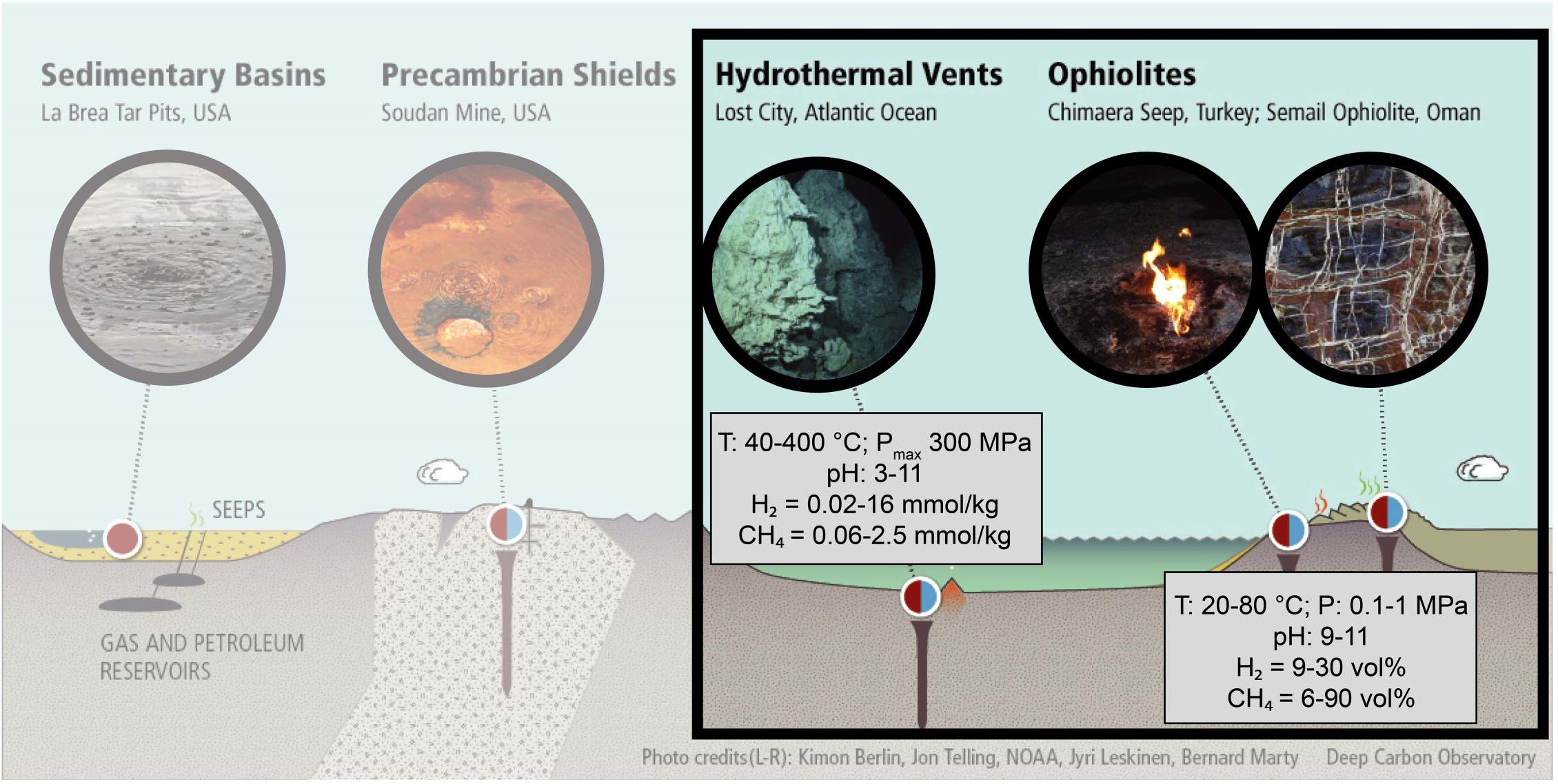
Figure 1. Geologic settings of intense H2 and CH4 degassing on Earth. The red and blue colors reflect the biotic and abiotic contributions, respectively, of which the relative fluxes are still under debate. The biotic production includes present-day microbial activity and thermogenic breakdown of organic matter from biological origin. The abiotic production results from radiolysis in Precambrian shields and serpentinization reactions at mid-ocean ridges or in ophiolites. Serpentinization settings are highlighted. (Credit: Josh Wood, modified with permission).
H2 production during serpentinization results from the oxidation of the ferrous component of ferromagnesian minerals (e.g., olivine, pyroxenes) coupled to the reduction of water (Thayer, 1966). In turn, H2 can reduce oxidized forms of carbon into CH4 and light hydrocarbons (HCs) via a Sabatier or Fischer-Tropsch-type (FTT) reaction (Szatmari, 1989). Industrial reactions use CO as the carbon source under gaseous conditions with metal catalysts to overcome kinetics hindrance, either Ru- or Rh-based and Ni-based for Sabatier and FTT reactions, respectively. However, the main source of oxidized carbon in natural systems is CO2, bi-carbonate, or carbonate ions depending on the pH, rather than CO, and reactions are likely to occur under aqueous conditions (McCollom, 2013). Consequently, the common use of Sabatier-type (R1) and FTT (R2) reactions among the geoscience community are:
4 H2 + CO2 = CH4 + 2 H2O (R1)
(3n + 1) H2 + n CO2 = CnH2n+2 + 2n H2O (R2)
The increased interest for these natural reactions over the last decades has led to a large number of thermodynamic modeling and experimental studies of serpentinization. Thermodynamic models using crustal conditions predict that H2 concentration at equilibrium with serpentinized peridotite increases with T and can reach hundreds of mM at optimum conditions (∼300°C) (Klein et al., 2009, 2013). This is close to the concentration expected near a reaction front, but an order of magnitude higher than those measured at oceanic vents (Andreani et al., 2013; Fouquet et al., 2013). CH4 is favored relative to CO2 with decreasing temperature and increasing H2 concentration, and should be the dominant C-bearing component in hydrothermal fluids released from serpentinization at temperatures below 400°C (Shock, 1992, Zolotov and Shock, 1999, 2000; McCollom, 2013), similar to observations in natural fluids (Figure 1). In experiments, the system tends toward equilibrium with time, but it is affected by kinetic effects that are related to a series of crucial parameters such as T, P, grain size, time, or fluid composition. Figure 2 shows a compilation of the H2 and CH4 concentrations produced during experimental serpentinization from the original dataset (Huang et al., unpublished). These concentrations agree with our understanding of serpentinization kinetics, displaying a higher H2 concentration in higher T experiments (>200°C) than in low T ones (<100°C) (Figure 2A), and also overlap with natural concentrations. Nevertheless, a detailed examination of Figure 2A reveals some discrepancies between results for ranges of T that are not easily attributable to parameters that affect kinetics, and questions the optimum conditions for H2 production. The situation appears much more complex and controversial when it comes to CH4 and HC production (Figure 2B). Although some experimental concentrations agree well with measurements for high-temperature (HT) fluids, the experimental trend displays an increase of CH4 as a function of T, which is opposite to the decrease expected from thermodynamic models. Moreover, experiments using 13C labeled sources, 13CO2, H13COOH, NaH13CO3, resulted in virtually no 13CH4 production (roughly two orders of magnitude below 12CH4) raising the issue of potential contamination by ubiquitous organic carbon in most experiments (McCollom and Seewald, 2001; McCollom, 2003, 2016; Foustoukos and Seyfried, 2004; Fu et al., 2007; Ji et al., 2008; McCollom et al., 2010; Lazar et al., 2012, 2015; Grozeva et al., 2017). These experiments have fueled questions about whether the abiotic synthesis of CH4 during serpentinization reactions actually occurs.
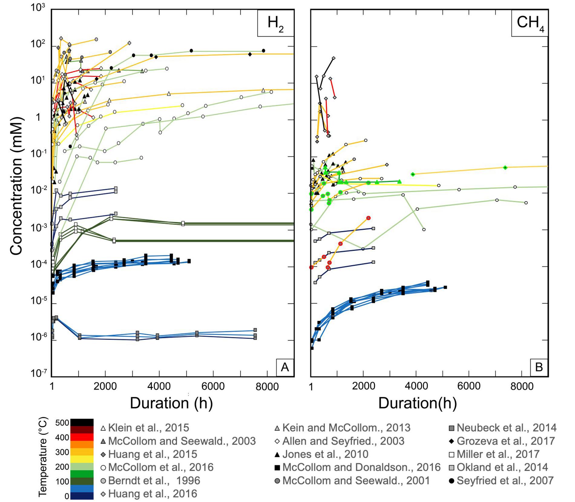
Figure 2. Summary of H2 (A) and CH4 (B) concentrations produced as a function of time and temperature during serpentinization experiments, in which duration can reach ca. 11 months. Concentrations span over eight orders of magnitude from nanomoles to hundreds of millimoles.
In order to feed the debate and achieve an unbiased reading of the available literature, we have built a comprehensive dataset of the experimental results of serpentinization available in the literature (Huang et al., unpublished), and, after dimensionality reduction, applied machine learning tools, a yet underused approach in geosciences. This approach provides an overview of the different conditions and protocols used so far, including the wide variety of experimental parameters that cannot be easily handled on regular plot (e.g., Figure 2). Finally, we discuss the variability of H2 and CH4 concentrations along with the consistency of the global dataset.
Data and Methods
Data Description
A large number of experiments have been conducted to study serpentinization, aiming at understand the abiotic production of H2, CH4, and other HCs during water–rock interactions (Berndt et al., 1996; Horita and Berndt, 1999; McCollom and Seewald, 2001, 2003; Allen and Seyfried, 2003; Foustoukos and Seyfried, 2004; Seewald et al., 2006; Fu et al., 2007, 2008; Seyfried et al., 2007; Ji et al., 2008; Dufaud et al., 2009; Jones et al., 2010; McCollom et al., 2010, 2016; Marcaillou et al., 2011; Neubeck et al., 2011, 2014; Lafay et al., 2012; Lazar et al., 2012, 2015; Klein and McCollom, 2013; Okland et al., 2014; Huang et al., 2015, 2016; Klein et al., 2015; McCollom, 2016; McCollom and Donaldson, 2016; Grozeva et al., 2017; Miller et al., 2017). The most extensive dataset compiled so far is described in a companion data paper (Huang et al., unpublished). This dataset includes serpentinization experiments in which minerals are initially introduced as reactants, as well as experiments run without solid reactants. The latter correspond either to blank experiments—designed to evaluate unavoidable contaminations (e.g., background carbon or H2 production)—or to relevant systems in which H2 levels would not be limited by mineral dissolution and could reach higher values, such as experiments with formate as a source of H2 and C.
The database (Huang et al., unpublished) indicates that the scientific community is mainly focused on two geological settings: ophiolites, characterized by low pressure (LP) and low temperature (LT) conditions (ambient or vapor saturation pressure, T < 100°C) and oceanic hydrothermal environments characterized by medium pressure (MP) to high pressure (HP) and HT conditions (30–300 MPa; 200–500°C). The highest pressures tested, at 350 MPa, are also relevant to shallow subduction environments where serpentinization occurs in the mantle wedge or fractured subducting lithosphere. There is a clear lack of data between 100 and 200°C, and between 50 and 300 MPa (Figure 3 and Supplementary Figure S1).
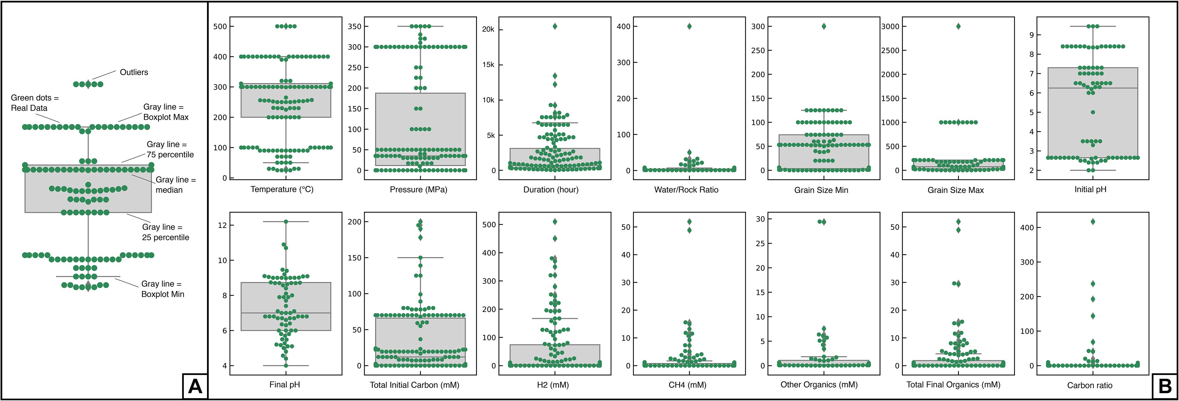
Figure 3. (A) Presentation of the general attributes of a swarm plot that helps to visualize the distribution of a selected data feature (green dots), e.g., temperature, H2, CH4, and related boxplots. (B) Swarm plots of the distribution of data according to experimental parameters and results analyzed in this contribution. The x-axis indicates the parameter, and values are plotted against the y-axis.
Various types of reactors were used to cover this large range of P-T conditions. For instance, gold cells in autoclave are common for experiments at HT (200–500°C) and HP (300 MPa) conditions (Huang et al., 2015, 2016; Lazar et al., 2015) while Parr type autoclaves, with or without flexible cells made of gold or titanium, are better suited for experiments at HT (200–500°C) and MP (30–50 MPa) conditions (Berndt et al., 1996; Horita and Berndt, 1999; McCollom and Seewald, 2001, 2003; Allen and Seyfried, 2003; Foustoukos and Seyfried, 2004; Seewald et al., 2006; Fu et al., 2007, 2008; Seyfried et al., 2007; Ji et al., 2008; Dufaud et al., 2009; Jones et al., 2010; McCollom et al., 2010, 2016; Marcaillou et al., 2011; Lafay et al., 2012; Lazar et al., 2012; Klein and McCollom, 2013; Klein et al., 2015; McCollom, 2016; Grozeva et al., 2017). Comparably, borosilicate glass bottles were preferred for LT and LP experimental conditions (Neubeck et al., 2011, 2014; Okland et al., 2014; McCollom and Donaldson, 2016; Miller et al., 2017). Figure 3 is a swarm plot showing the number of data points in green of a given value for a series of selected parameters. The gray box represents the 25–75th percentile and the gray line is the median value. The gray lines outside the box represent the minimum and maximum values, with the exception of outliers. P, T, and initial/final pH of the fluid follow a bimodal distribution that mimics the natural conditions illustrated in Figure 1. Addition of NaCl or NaHCO3 salts, presence of catalyst, and gold capsules are the most frequent features in the dataset, used in more than 50% of experiments. This indicates that inorganic carbon in experiments is most often introduced as NaHCO3 salt, and that the most classical reactors are made of gold. Other dataset features are highly variable, for example, all experiments have their own starting materials (e.g., mineral assemblages, fluid compositions), sample volumes that range from 0.05 to 180 mL, and experimental run durations from hours to a year.
The complete dataset (Huang et al., unpublished) includes more than 100 parameters. Each column represents a feature, such as an experimental parameter, reactant, or product, and each row is a measurement. Some of the 100 features of the complete dataset are too sparse to allow running data analysis algorithms directly. Hence, in the present study, we performed dimensionality reduction by removing the less variable parameters and combined some features to increase data density within 37 features in a working dataset (Table 1). Hereafter, we will refer to the header of the column that is an explicit shortcut for its content. For example, the “Other_organics” feature sums all organic products except CH4; the “Fe_bearing” feature combines all Fe-bearing solids (synthetic or natural) added to the system (e.g., FeO, hematite, sulfides) except olivine and magnetite, which are considered as independent parameters. Some experiments include multiple samplings as a function of time and had more than one measurement (as shown in Figure 2); in these cases, only the final measurements were kept for the analysis in order to prevent overweighting those experiments in the analysis. Hence, the final working dataset includes 158 measurements in total, which result from experimental runs with different durations.
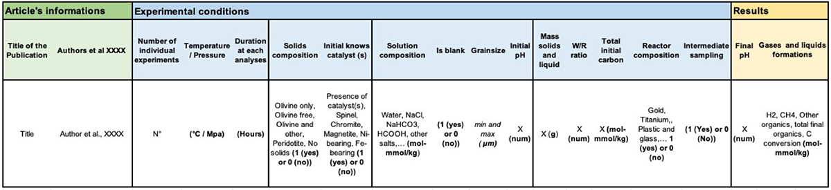
Table 1. Description of the working dataset modified from Huang et al. (unpublished) organized in three major sections: article’s information (green), experimental conditions (blue), and results (yellow).
Pearson Correlation Coefficient Matrix
The Pearson correlation coefficient is a value between -1 and 1 that indicates the extent of linear correlation between two variables. A coefficient of -1 or 1 means the two variables are in perfect negative or positive correlation respectively, with 0 indicating no correlation. Details of how the coefficient is calculated can be found in Pearson (1895) and Lee Rodgers and Alan Nice Wander (1988). The pairwise Pearson correlation coefficient matrix for our final dataset is calculated and displayed in Figure 4.
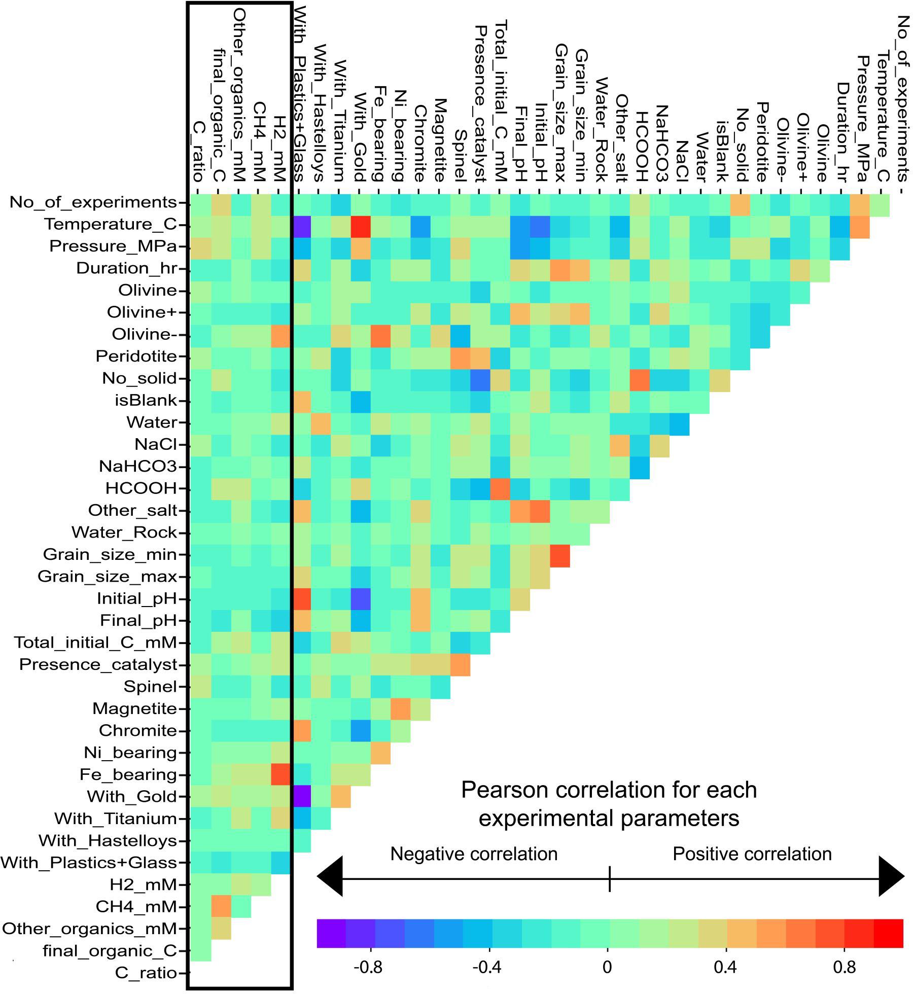
Figure 4. Pearson correlation coefficient matrix between all parameters analyzed in the dataset. Warm and cold colors show positive and negative correlation, respectively. The black rectangle across the first five columns highlights the five important experimental products.
It is worth noting that some parameters are dependent and led to some of the strongest correlation, e.g., between “CH4,” “Other_organics,” and “Total_final_organics,” the latter being the sum of the formers. Another example is “Spinel,” which correlates with “Peridotite” and “Presence_catalyst” because peridotite is partly composed of spinel and spinel is a common catalyst of some reactions. Conversely, “Magnetite,” which was separated from the “Fe-bearing” and “Spinel” lists, does not correlate with “Fe-bearing” and “Spinel.”
The experimental protocol also induced some strong correlations. For instance, temperature is strongly positively correlated with the parameter, “With_Gold,” and negatively correlated with the parameter, “With_Plastics+Glass,” classically used for HT and LT experiments, respectively. Similarly, the use of formate, “HCOOH,” as a source of carbon and H2 is strongly correlated to the highest levels of initial carbon, “Total_Initial_C_mM,” which are used in the gold reactors (“With_Gold”) predominantly in experiments that did not include mineral phases (“No_solid”).
The black box (Figure 4) highlights the correlations of interest, i.e., between all parameters, H2, and carbon products. It shows the lack of strong correlations that prevent the interpretation of the database using conventional wisdom. These relationships are presented and discussed in Section “Results and Discussion,” with the help of network analysis.
Network Analysis
Network analysis is a collection of analytical and visualization methods that have been employed to study complex systems in various fields of science and technology. For example, in biology, it has been applied to the study of ecosystem diversity (Banda-R et al., 2016), proteomics and protein–protein interactions (Amitai et al., 2004; Harel et al., 2015), evolution (Vilhena et al., 2013), and mass extinction events in Earth’s history (Muscente et al., 2018, 2019). In urban planning, networks have been used to model power grids (Pagani and Aiello, 2013), roads (Dong and Pentland, 2009), and water supply systems (Geem, 2006) as well as communications infrastructure (Hansen and Smith, 2014). Networks of people have also featured prominently in the study of social media, the spread of infectious diseases, the structure of criminal organizations, and connections among research collaborators (Otte and Rousseau, 2002; Abraham et al., 2010; Eslick, 2012; Scott and Carrington, 2015).
The power of network analysis arises mainly from its capability of representing and visualizing large sets of highly dimensional data and exposing the complex relationships amongst them. Entities are represented by nodes (vertices) and are connected by edges (links) that illustrate the relationship between entities. The visual attributes of the nodes such as shape, color, or radius, and of edges such as weight (line thickness), can be mapped to values resulting in a dynamic and more expressive network diagram. Visual inspection of the diagram with some perturbation of the parameters is a powerful tool for revealing potentially unseen patterns and characteristics in the data. A number of quantitative analytical techniques can be applied to the network in order to study and quantify the significance of these patterns and behaviors.
In this methodology, the nodes refer to each experiment within the dataset, and edges represent the similarity between different experiments. Therefore, nodes that cluster together have short edges, and represent similar experiments. At the end of the analysis, a cluster of nodes then becomes a community of similar experiments. The method to calculate similarity scores is explained in the following section.
Cosine Similarity Matrix
The network is built from a pre-calculated cosine similarity matrix (Janbandhu and Karhade, 2015). Each experimental measurement can be treated as a 35-dimension numeric vector (37 experimental features minus two article information features), and the pairwise cosine similarity score is calculated between each vector. The cosine similarity scores between two experimental features represent the combined effect of all parameters and vary between −1 and 1.
In the working dataset, 0 stands for no and 1 for yes, for categorical values. Numerical values such as temperature, pressure, or durations were normalized between 0 and 1 to avoid biases due to different value ranges. We then used the similarity scores as the edge weights of the networks. Since we consider just serpentinization experiments, many studies have some parameters in common, which results in a fully connected network with varying edge weights. Even though a fully connected network contains abundant information and potential insights, we choose to optimize the efficiency of the community detection algorithms by choosing a threshold to eliminate edges with low importance. For this purpose, we ran experiments by eliminating edges with low similarity scores and testing their effects on the results of the community detection algorithms.
Fruchterman–Reingold Force-Directed Networks
The Fruchterman–Reingold force-directed graph algorithm (Fruchterman and Reingold, 1991) simulates attractive and repulsive forces between the nodes, similar to those of molecular or planetary simulations, while attempting to find a minimum energy state for the network layout. It is based on two general principles: (1) nodes connected by an edge should be drawn near each other and (2) nodes should not overlap. To compute the layout, the method iteratively adds nodes to the diagram while recalculating the attractive and repulsive forces and displacing existing nodes accordingly. As such, we do not control the lengths of the edges or the final positions of the nodes, which are determined when the system reaches equilibrium. In this study, we use a python package called Networkx (v. 2.3) (Hagberg et al., 2008) to build the network. The 3D network structure is fixed by this algorithm, but its 2D projection can change at different angles randomly, meaning that every time when we run the code, the 2D project will change. For any algorithm involving randomization, a seed can be used to make the algorithm produce consistent results. We tested a set of seeds from 0 to 200 and found that seed 103 gives the clearest and most informative layout for our data. If the reader wants to reproduce our results, please use the same seed number as ours.
Louvain Community Detection Algorithm
The Louvain community detection algorithm (Blondel et al., 2008) attempts to find community structure in a network through multi-level modularity optimization. Initially, each node is assigned to its own community. At each step, nodes are reassigned to the communities with which they achieve the highest contribution to modularity. When no more nodes can be reassigned, the process is applied again to the merged communities and is stopped when there is only a single vertex remaining or modularity cannot be further improved. The algorithm in this paper is implemented using a package called python-louvain1.
Results and Discussion
Detection of Four Communities of Experiments: A Snapshot of the Literature
The Pearson similarity matrix (Figure 4) built from our dataset revealed no clear trend between experimental parameters and reaction products. It mostly identifies a couple of strong and inevitable correlations between some experimental parameters, such as the use of gold cells for HT experiments (see section “Pearson Correlation Coefficient Matrix”). However, it confirmed that (despite some trends on the kinetic curves that could already be drawn using the complete database; Figure 2), data discrepancies cannot be easily interpreted using conventional wisdom. We used the parameters reported from each experiment in our dataset to build a cosine similarity matrix, and then constructed a network (see section “Data and Methods”) with a layout defined by Fruchterman–Reingold force-directed graph algorithm. Four communities were detected using the Louvain community detection algorithm, as colored distinctively in Figure 5A, and plotted individually in Figure 5B. These experimental communities present overall similarity among different experiments when taking into account all experimental features, including starting materials, reactants, reactors, fluids, reaction products, and potential catalysts. Hence, they provide a full “picture” of the available literature, i.e., the conditions that have been explored to date and the degree of similarity or dissimilarity of the results. For ease of comparison, the network diagrams presented in Figure 5 follow the same color chart and layout throughout the manuscript.
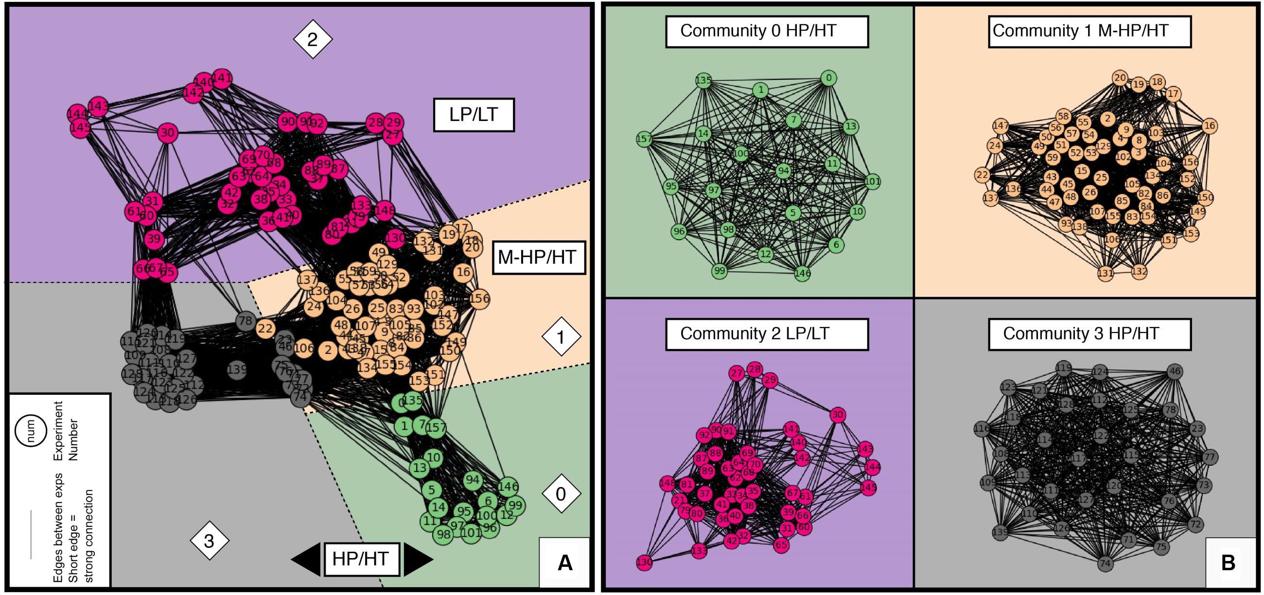
Figure 5. Networks built with the cosine similarity matrix calculated from the dataset, with the four detected communities that are a snapshot of the conditions tested so far and their usual experimental protocols (community 0: HP/HT using HCOOH as a source of C and H2, community 1: M-HP/HT, community 2: LP/LT, community 3: HP/HT with C_ratio > 1) (see Figures 6, 7). (A) The full network. Each filled circle (node) represents an experiment, which number is included and allows to back track the corresponding experiment in the database. The shorter the link (edge) between two circles, the higher the correlation between the experiments. (B) The four separate community networks. Communities have been arbitrarily color coded as a guide for the eyes, which remained the same in all figures—green, brown, purple, and gray, for communities 0, 1, 2, and 3, respectively.
The cosine similarity threshold and the initial node have been tested before ending up with these four experimental communities. Supplementary Figure S2 shows that by successively removing the weakest 10, 30, 50, and 70% of the edge connections, the communities detected by Louvain algorithm are quite similar. We therefore infer that these communities are robust and represent real trends in the data. The number of communities detected is always four, and communities 0, 1, and 3 virtually stayed the same. When we remove the weakest 70 % of edge connections, nodes 143, 144, and 145 in community 3 moved into community 2.
Our analysis enabled us to find the optimum threshold (0.39) where the community detection algorithms produce very similar results to the densely connected networks, while increasing the efficiency of the network. This approach assisted in identifying the important edges in the network structure. Depending on the initial node chosen by the algorithm, the number of detected communities was dominantly four but could increase to five occasionally. The initial node is chosen randomly by the algorithm, and the random state can be set with a random seed. As explained in Section ““Fruchterman–Reingold Force-Directed Networks,” if you want to reproduce the layout of our plots, please use a seed of 29. As the random seed varied, community 0 always remained the same, but a few nodes on the edges of communities 1 and 2 (e.g., node 143, 144.), and 1 and 3 (e.g., node 22, 46, 106) would change.
In order to identify the main features that control the separation into the four communities identified with Louvain algorithm, we colored the nodes of the network as a function of the value of each experimental parameter. For parameters with binary values, white and lemon colors were used for 0 and 1, respectively. Red stands for unreported values. Selected plots are displayed in Figure 6; others are available in Supplementary Figure S3. This data analysis highlights the primary control of temperature (T) and pressure (P) on the experimental communities (Figures 6A,B), akin to natural end-member conditions (Figure 1). Community 2 clearly corresponds to LP/LT experiments at ambient P and T below 100°C, while the other communities encompass experiments run at higher P and T. Community 1 differs from communities 0 and 3 because of pressure and covers MP range between 10 and 100 MPa. Community 3 differs from community 0 and others because it contains experiments that exclusively used the decomposition of formic acid HCOOH as a source of H2 and CO2 and buffered the initial pH to the lowest values reported in the literature (Figures 6C,D). Community 3 also lacks information on the water-to-rock ratio since neither a solid phase (Figure 6E and Supplementary Figure S3A), nor NaCl was added to the fluid (Supplementary Figure S3B), distinguishing it from almost all other experiments. It is worth noting that except for experiments performed with HCOOH, initial pH values are rarely reported in experiments within communities 0 and 1, and are most likely close to neutral or slightly alkaline considering the presence of NaCl with or without NaHCO3, respectively. Visualization of community 2 shows that LP/LT experiments have also been run at neutral to basic conditions to mimic outflow fluid composition in ophiolitic settings. Hence, experimental results of community 3 cannot be directly compared to the others and will be plotted in the following graphs for informative purposes only. Detailed examination of the communities’ characteristics highlights the lack of experiments under initial acidic conditions that are supposed to be the most favorable for olivine dissolution (Oelkers, 1999; Kaszuba et al., 2013). This might be due to the fact that natural serpentinizing systems are not expected to be acidic at a temperature of or below 300°C. However, reaction with acidic HT hydrothermal fluids such as those escaping from peridotite-hosted hydrothermal vents at slow-spreading ridges can occur (Fouquet et al., 2013). Finally, analysis of the communities shows that the initial fluid composition is a feature that has never been explored so far, especially in HT experiments.
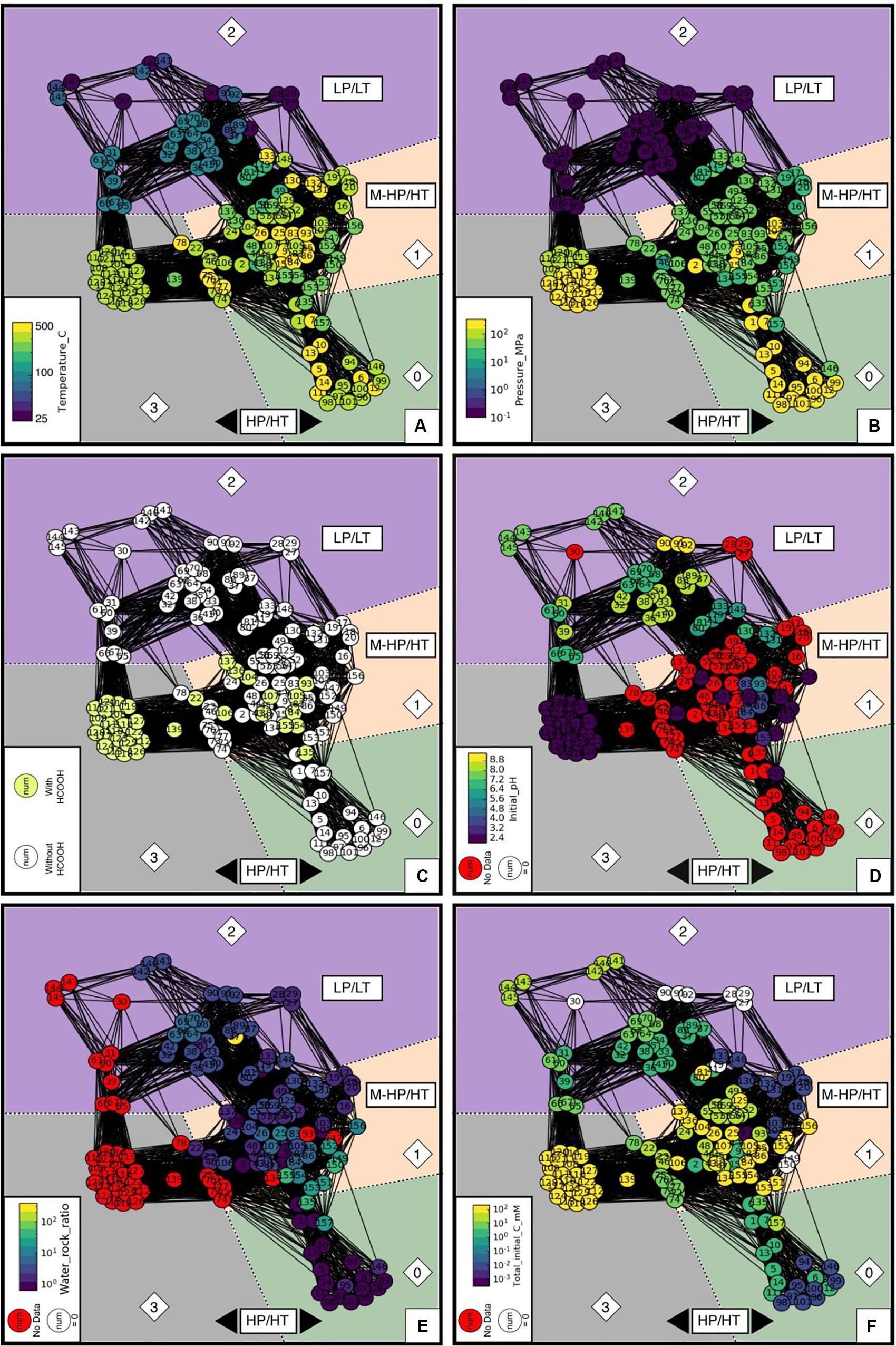
Figure 6. Values of the parameters that dominantly control the distribution of the data in four different communities of experiments: (A) temperature in °C; (B) pressure in MPa; (C) presence or absence of formic acid in the starting aqueous solution, with or without HCOOH; (D) pH of the starting aqueous solution (Initial_pH); (E) relative amount of water and rock (Water_rock_ratio); and (F) the total initial carbon concentration in the starting aqueous solution by adding up all carbon species (Total_initial_carbon_mM). All red filled circles indicate that the value of the parameter is missing in the original article that presents the experiment.
When looking at individual communities (Figure 5B and Supplementary Figure S4), experiments are also well grouped into clusters of LP/LT, MP/HT, and HP/HT conditions, even if P and T only partially characterize the communities. Communities 1 and 3 contain the highest number of nodes while community 0 is the smallest one, illustrating the limited number of experiments run at the pressure of hundreds of MPa. Communities 0, 1, and 3 form round layouts, whereas the layout of community 2 is irregular. Considering the layouts are defined by the force directed algorithm, this analysis indicates that the diversity of experimental parameters, notably fluid composition, is generally much larger in LP/LT experiments (community 2) than in others. For example, this is visible when looking at the variety of initial pH values, “other_salts” (e.g., MgCl2, CaCl2), or water-rock ratio tested under ambient pressure and temperature below 100°C (LP/LT).
H2, CH4, and Hydrocarbon Production
Figure 7 shows the distribution of the concentrations of gaseous H2, CH4, and other organics together with the carbon ratio (“C_ratio”) among the four communities. The C_ratio is the ratio between the carbon initially introduced in the system and the final measured one, according to the available information. This cannot take into account the potential carbon contamination of reactants that has never been quantified by the authors of the publications analyzed in the database. The distribution of H2 concentrations across communities is bimodal, spans eight orders of magnitude, and correlates with temperature (LT versus HT) but not pressure (Figure 7A) with the exception of community 3, whose experimental production of H2 was not reported. CH4 concentration spans five orders of magnitude and correlates with both T and P (Figure 7B); production is lower at LP/LT (community 2) than at HT (communities 1 and 3), and the highest concentrations are clustered in community 0 at HP. Community 0 is also characterized by “C_ratio” values higher than one (Figure 7D), which are unrealistic and necessitate that an unidentified source of carbon was present in the system, hence indicating contamination issues with the samples. It may also be responsible for the occurrence of other organic products (“Other_organics”), which systematically occur in community 0 (Figure 7C) and are occasionally observed in the others. Therefore, we will not discuss the results of community 0 further.
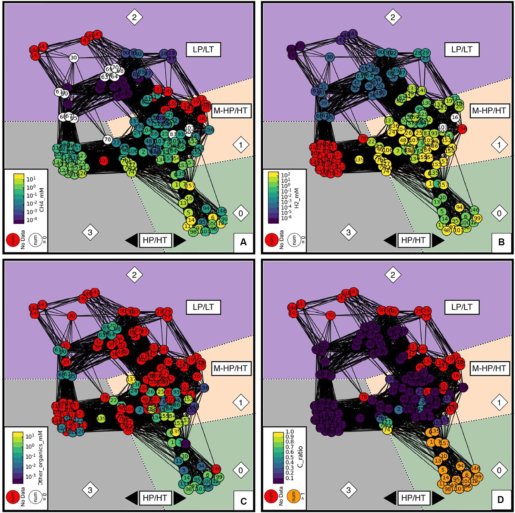
Figure 7. Networks of concentrations of: (A) CH4, (B) H2, and (C) other organic species. The heatmap color from cold to warm corresponds to low to high concentrations. Red nodes refer to experiments that did not report relevant concentrations. Experiments labeled in white have concentrations below detection limits, which are set to 0 in the database. (D) C_ratio - total final carbon divided by total initial carbon. Theoretically, C_ratio should be between 0 and 1. Dark purple nodes are experiments that did not include or report initial carbon concentrations (set to 0 by convention). Red nodes refer again to final carbon concentrations not reported in the original literature. The orange nodes, mainly in community 0, are experiments reports more final carbon than initial carbon, i.e., C_ratio higher than 1. This suggests that those experiments might have undocumented contamination issues.
Figure 8 further illustrates the evolution of H2 and CH4 concentration as a function of P and T together with values from 13C-labeled and blank experiments. As our dataset only considers the last sampling point of each experimental set (see section “Data Description”), the experimental duration varies from one data point to another. Hence, we also plot H2 and CH4 concentration as a function of duration (Figure 8C) to check whether the variability observed at a given P or T does not simply result from experimental duration (reaction kinetics). Figure 8 confirms the overall trends depicted on Figure 2 (regular kinetic curves using the non-reduced database) for both H2 and CH4 distribution and better highlights the strong variability of concentrations for given P-T conditions. The lack of consistency of the whole database is confirmed by the absence of correlation between gas concentrations and duration when observing all final experimental points from different experiments (Figures 8C,F). It is worth noting that blank experiments are frequently reported at LP/LT, while none are available at higher T to establish background levels of H2 and CH4 under those conditions. Experiments starting with 13C labeled sources have been used instead to test carbon contamination issue in a limited number of experiments (triangle symbols in Figure 8), but background levels of H2 remain unknown to date.
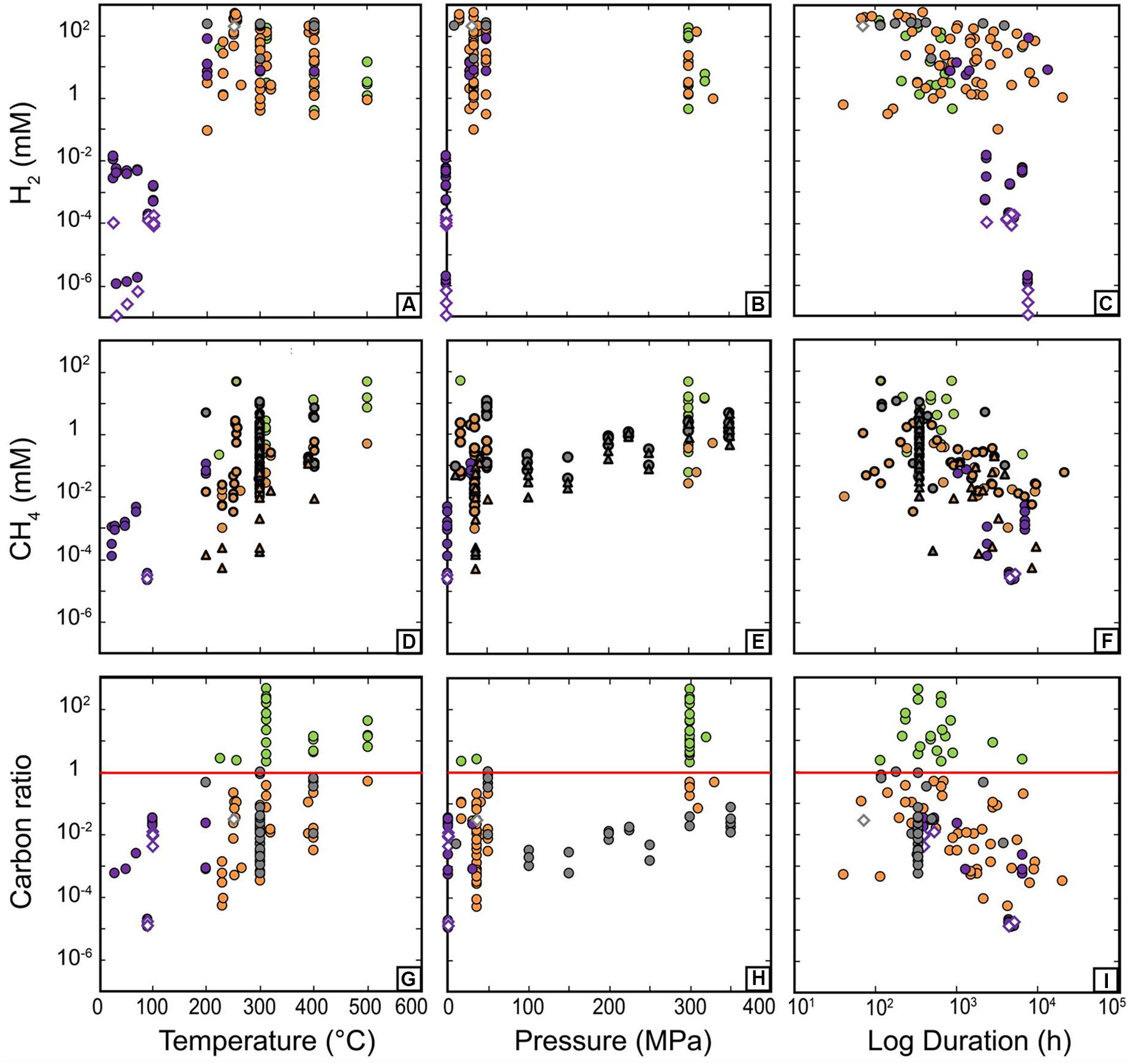
Figure 8. Concentrations of H2 (A–C), CH4 (D–F), and carbon conversion (G–I) displayed as a function of temperature (A,D,G), pressure (B,E,H), and experiment duration (C,F,I). Diamond symbols correspond to “blank experiments” run without minerals in the experimental load. Thick triangle symbols in (D–F) highlight 13CH4 concentration while thick circles show the corresponding total CH4 also including 12CH4. In (G,H), the red line corresponds to a carbon ratio value of 1, beyond which is suspected to be contaminated. Color coding consistent with Figure 5.
The evolution of H2 concentration as a function of P and T (Figures 8A,B) also highlights two regimes of reaction, at LP/LT below 100°C in the MPa range, and at MP–HP/HT above 200°C. In the LP/LT regime (community 2), H2 concentration is low, between 10–1 and 10–3 mM, and blanks indicate that concentrations below micromolar are not significant. In the MP–HP/HT regime (communities 0, 1, and 3), H2 concentrations can almost reach molar concentrations. HCOOH-bearing experiments (community 3) always have the highest values reported. This is expected because in these cases H2 comes from the decomposition of HCOOH that was introduced at high concentration (10–100 mM) in the starting fluid. In the other groups where H2 results from redox reaction with iron-bearing phases, H2 concentration is highly variable and no sweet spot for H2 production could be identified, hence preventing the description of a trend with either T or P (Figure 7). This does not correlate with serpentinization kinetics deduced from solid phase transformation (olivine-to-serpentine transformation, Martin and Fyfe, 1970; Malvoisin et al., 2012; McCollom et al., 2016). Indeed, serpentinization kinetics classically display a bell curve with a maximum at ∼250–300°C that is not observed in the current H2 dataset. H2 concentrations are neither correlated to duration nor to grain size (Figure 4). Available data on initial pH (Figure 6D) are too scarce to be conclusive. Rather, Figure 4 shows that H2 concentrations display strong positive correlation with “Olivine-” (i.e., olivine-free run) and “Fe_bearing” features, which are highly correlated to each other as well. This suggests that the highest levels of H2 are reached with a source of Fe (0 or II) other than olivine, i.e., derived from Fe-bearing species such as Fe-bearing salts, oxides, or alloys. Olivine, whose iron content is lower and whose release in the fluid is controlled by dissolution kinetics, appears less efficient at producing H2 than the other iron-rich compounds. However, this does not explain the variability among serpentinization experiments [i.e., the olivine-bearing experiments (“Olivine” and “Olivine+”) that dominate the database (e.g., Figure 2)]. It is worth noting that H2 also positively correlates with the presence of catalysts “Presence_catalyst” (Figure 4), whose occurrence is widely distributed among all communities (Figures 10A–D) suggesting either a catalytic or a reactive role of these phases on the production of H2 (see section “Effect of Accessory Solid Phases” for details).
In order to produce abiotic methane, assuming that it forms by an FTT reaction, an oxidized form of carbon is often added to the starting fluid. The CH4 concentration is then measured (Figure 2B) at the end of experiments. The evolution of CH4 evolution as a function of P and T (Figures 8D,E) first shows that CH4 concentrations are one to two orders of magnitude below those of H2 (Figure 9A). Figures 9B–D show that CH4 concentrations are also well below the concentrations of the oxidized carbon sources deliberately introduced in experiments, except for community 0 which was removed from discussion because of an unrealistic “C_ratio” (Figure 7D). First, this indicates that the low CH4 concentrations do not result from limited reactant availability for reaction R1. Second, it suggests that CH4 formation by reduction of oxidized carbon forms, if possible, is not efficient and far from equilibrium. Only LP/LT experiments displaying the lowest values of methane concentration achieve values close to expected CH4 concentrations (Figure 9A). These low methane concentrations, near micromolar level, are still above those of blank experiments run at similar conditions. At high T, 13C-labeled experiments report undetectable to micromolar levels of 13CH4, whether catalysts are present or not (see section “Effect of Accessory Solid Phases”). These concentrations are well below the CH4 concentration measured in all other experiments (Figures 8D–F, 9B–D). Assuming that the use of a heavy carbon source in 13C-labeled experiments does not have a kinetic effect on carbon reduction reactions, these results indicate that abiotic CH4 has never been formed at a significant level during serpentinization experiments. As such a strong statement rules out most of—if not all of—the available literature we further investigated the present database to discuss this hypothesis (see section “Contamination Issues”) and investigated the consistency of the available data for actual CH4 production by an FFT process.
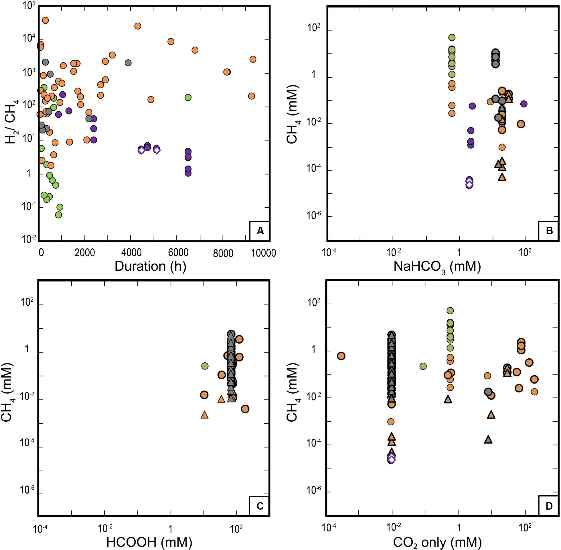
Figure 9. (A) H2/CH4 ratio as a function of time. CH4 concentration as a function of the initial carbon sources in experiments (bi-)carbonate salts (B), HCOOH (C), and CO2 (D). Thick triangles and circles correspond to labeled 13CH4 and total methane, respectively. Color coding consistent with Figure 5.
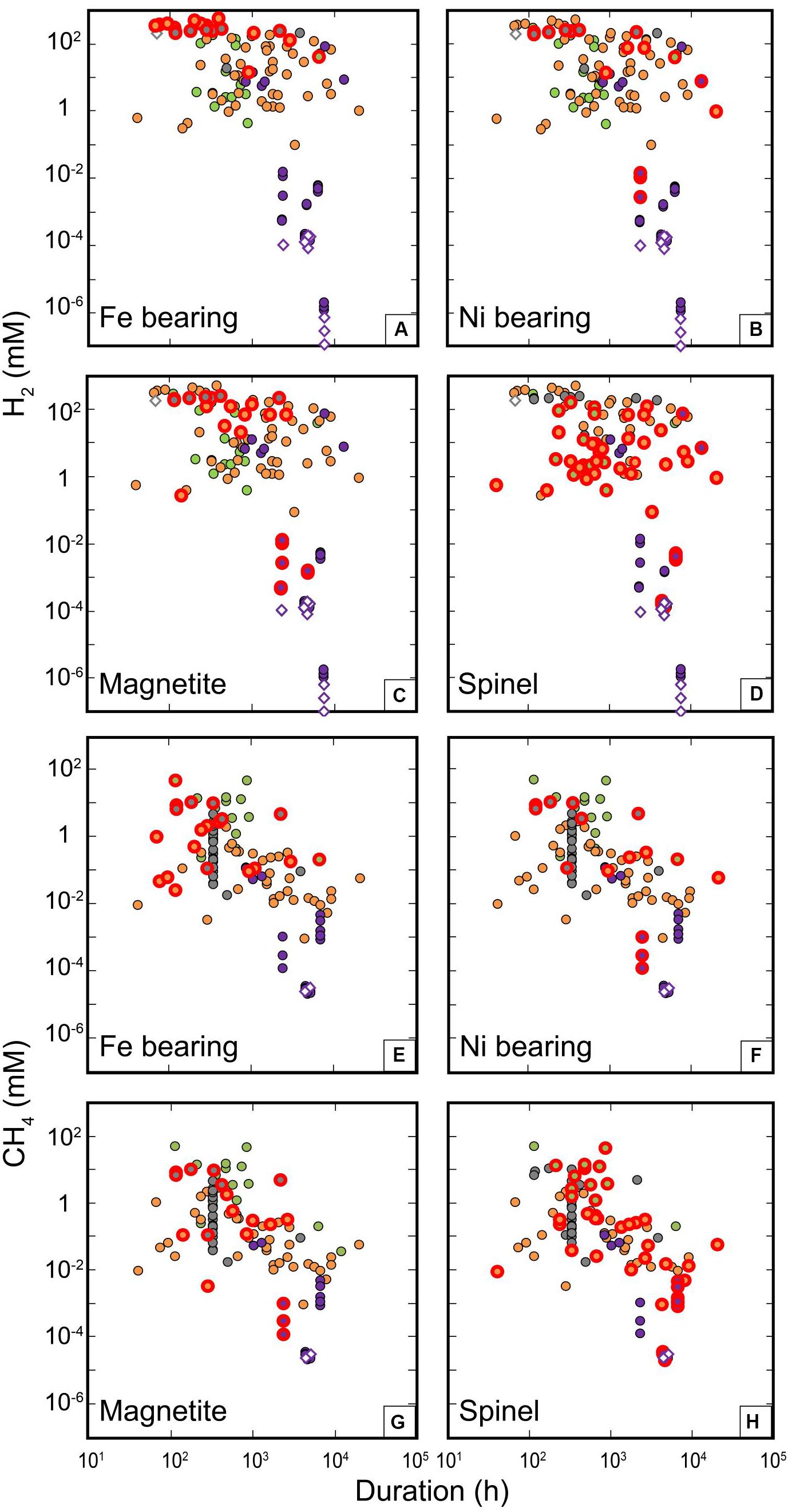
Figure 10. Potential catalytic effects on the formation of H2 and CH4. Concentrations of H2 (A–D) and CH4 (E–H) are plotted against run durations. Diamond symbols correspond to experiments without initial mineral phases, and red thick circles highlight the experiments with relevant catalyst reactants. (A) “Fe-bearing” ones include metallic iron, hematite, Ni-Fe alloys, FeS, FeO except magnetite; (B) “Ni-bearing” ones include NiS, Ni-Fe alloys; (C) “Magnetite” corresponds to experiments with magnetite; (D) “Spinel” corresponds to experiments with spinel or spinel-bearing peridotite. Color coding consistent with Figure 5.
The dataset shows that CH4 concentrations display a logarithmic increase with T between ambient T and 500°C (Figure 8D) and they do not show any dependence on pressure above 30 MPa. The increase of CH4 concentration with T is also well highlighted by the 13C-labeled experiments, despite much lower 13CH4 concentrations. The strong variability of CH4 concentrations among experiments from the largest community (community 1) precludes any further correlation between CH4 and pressure. Figure 8F highlights that duration does not account for the variability of CH4 concentrations in experiments at given P-T conditions. The same holds for “grain_size,” which is uncorrelated with CH4 concentrations (Figure 4).
McCollom et al. (2010) suggested that the nature of initial carbon source may affect the system reactivity, and they showed that dissolved CO and HCOOH carbon sources are more effective at abiotic organic synthesis than CO2. We test this hypothesis by comparing the CH4 concentrations reached for the different types of carbon source ((bi-)carbonate salts, HCOOH, or CO2) (Figures 9B–D). This selection of carbon sources is not the choice of the authors, it simply reflects the C-sources reported in the publications. HCOOH-bearing experiments (mainly community 3—all run at similar T conditions), in which high amounts of HCOOH have been added (10–100 mM), produced the highest CH4 concentrations (∼10 mM) at HP (Figures 8D,E, 9C), excluding data from community 0 because of contamination issues. Such experiments, in which olivine is mostly absent and HCOOH decomposes to H2, CO2 (±CO) at HT, are reported here for comparison but are not representative of the actual serpentinization process investigated so far in experiments. Experiments of community 2 at LP/LT have only used NaHCO3 at one concentration and show variable CH4 production. It appears that the most comprehensive dataset for this discussion is provided by the experiments in community 1 at MP–HP/HT. In community 1, CH4 concentrations display an overall correlation with CO2 content, which is also evidenced in 13C-labeled experiments for lower CH4 concentrations. Such a correlation is not observed with initial NaHCO3 concentrations whose variation range is too limited. This precludes the comparison between the reactivity of carbonate/bicarbonate ions versus CO2.
The above observations show that despite considerable efforts, the available experimental dataset remains incomplete and limits the analysis. Nevertheless, results deeply question the potential of these carbon sources to efficiently react with the H2 derived from serpentinization, and suggest a strong inhibition of R1 under those conditions, even with high reactant concentrations. In addition, the increase of CH4 as a function of T (Figure 8D) does not follow thermodynamic predictions and rather indicates a kinetic or a thermal control of experimental CH4 production, whatever the reaction is. The only plausible trajectory toward equilibrium is observed for LP/LT experiments (community 2, Figure 9A) and may be related to the presence of a gaseous phase in most of these experiments run into incubation flasks, i.e., in conditions closer to those ideal for reactions R1 and R2. The potential importance of a gaseous phase that could be mandatory for CH4 production was already raised by some authors and deserves further investigation (Etiope et al., 2011; McCollom, 2013).
Data on the production of organic products other than methane are very sparse and were combined in the dataset into a feature called “Other_organics” (Figure 7C) that dominantly includes small organic molecules (<0.1 mM) measured in either the liquid phase at LP/LT (organic acids, community 2) or the gas phase at MP/HT (HCs, communities 1 and 3). These sparse data do not show any obvious correlation with CH4, as possibly expected from reaction R2 (Figures 4, 7C). Figure 4 rather points to a positive correlation between “Other_organics” and “Total_inital_C” that is potentially true for the whole P-T range since “Other_organics” (mainly in the form of organic acids) were also detected at LP/LT conditions in the aqueous phase while CH4 was not.
Effect of Accessory Solid Phases
Metal-bearing catalysts are critical to the industrial production of H2 or CH4 in gaseous phase. Notably they are critical for (R1) and (R2) to overcome the first step of CO2 reduction to CO by the water-gas shift reaction. The lack of data on CO occurrence and concentration in hydrothermal experiments focusing on serpentinization does not allow either decomposing reaction mechanisms or discussing the potential role of CO as an intermediate phase, which has been examined by a previous experimental study (Seewald et al., 2006). In addition, under aqueous conditions, the catalytic phases can be more reactive and propitious to alteration and consequently act either as real catalysts (do not react but accelerate the reaction) or as reactants whose transformation directly produces H2 (e.g., alloy) or facilitates olivine dissolution, such as aluminum (Andreani et al., 2013). Addition of any material in a reactor also induces potential introduction of carbon contamination that could contribute to gas production.
To distinguish the role of potential catalysts, an in-depth characterization of the solid surfaces before and after experiment is mandatory. Unfortunately, this step has not been done in the large majority of experiments, hence preventing any inference. This also precludes the potential identification of precipitated carbonaceous phases among solids (Milesi et al., 2015; Andreani and Ménez, 2019). Here we take advantage of the dataset to discuss potential correlation between the concentration of reaction products such as H2, CH4, or the other organics, and the presence or absence of potential catalysts in experiments for guiding future studies. The list of potential catalysts includes those introduced in the experiments as solids, natural or synthetic, such as Cr-spinel, magnetite, chromite, Ni- or Fe-bearing minerals or alloys. It also includes those produced by the serpentinization reaction such as magnetite or spinel, that have a recognized significant effect on the reaction. For example, spinel has been shown to improve H2 production at LP/LT (Mayhew et al., 2013). We also do not underestimate the potential catalytic role of the constitutive materials of the reactor vessels commonly made of Au, Ti of HastelloyTM (a Ni/Fe-bearing alloy), whose catalytic properties have been demonstrated for some other reactions notably in aqueous systems, for example, CO2 reduction to CO (Chen et al., 2012), reforming reactions (Van Haasterecht et al., 2014), H2 production (Michiels et al., 2018; Fowler et al., 2019), and HCOOH dehydrogenation (Brunet and Lanson, 2019). Despite such evidence, especially for Au and Ti which are the most used for studying serpentinization reactions, reactor vessels are classically considered as inert for geochemical experiments dedicated at understanding the potential of serpentinization to produce abiotic H2, CH4, and light HC.
In the previous section, we highlighted the positive correlations between H2 and the presence of potential metal catalysts (“Presence_catalysts”). A more detailed examination of Figure 4 shows a positive correlation between H2 production and the following catalysts, in decreasing order: “Fe-bearing” > “Titanium” > “Au” ∼ “Ni-bearing” > “magnetite.” “Chromite” and “Hastelloy” have no correlation and “Spinel” a potentially negative one with H2. The case of titanium reactors is well known as Ti-reactors have to be pre-oxidized prior to hydrothermal experiments in order to avoid H2 production from Ti oxidation (Seewald et al., 2006) and we reasonably assume that this step was run before experiments. Hastelloy, gold, or Ti do not have any recognized catalytic properties for H2 production or CH4 formation, and the strong correlation between H2 concentrations and gold or titanium could also well be due to the fact that H2 production is intrinsically more efficient at MP-HP/HT in hydrothermal reactors that are systematically made of gold and titanium. Hence, it is not yet possible to disentangle between P-T and catalytic effects here. Figure 10 shows the concentrations of H2 as a function of experimental duration for experiments run with the catalysts usually considered as the most optimal, i.e., omitting reactor metals and spinel, the latter displaying a slight negative correlation with H2. Figure 10 fits well with the ordering of potential catalysts previously identified on Figure 4 (“Fe-bearing” > “Ni-bearing” > “magnetite”). Irrespective of the run duration or the community, the addition of “Fe-bearing” phases that encompass both Fe(II) and Fe(III) compounds appears to be the most efficient and leads to the highest production of H2 (Figure 10A). A strong contribution of Fe(II) oxidation is expected in most cases but there may be underappreciated effects of Fe(III)-bearing phases yet to be explored in future works. H2 synthesis is also clearly enhanced by the presence of Ni-bearing phases at MP/HT conditions (community 1) while magnetite seems to be efficient for both LP/LT (community 2) and MP/HT conditions (community 1). As for “Fe-bearing” phases, oxidation of Fe(II) in magnetite and of Ni or reduced sulfur in Ni-bearing phases such as alloys or sulfides may intrinsically produce more H2 without a true catalytic effect occurring. Indeed, moderate amounts of Ni metal particles have recently been identified as catalysts of FeO oxidation under hydrothermal conditions (Michiels et al., 2018) and this effect may be extrapolated to Fe-bearing minerals such as olivine (Brunet, 2019). Conversely, H2 concentrations in spinel-bearing experiments cover the whole range of concentrations despite run duration or P-T conditions (all communities) and always lie below the maximum values observed, which explains the negative correlation observed in Figure 4. Hence, spinel does not appear as a good candidate for catalyzing H2 production under those conditions. The effect on H2 production of those different phases often introduced in experiments contributes to the variability of concentrations observed for similar thermodynamic conditions, whatever the mechanisms behind.
The correlation between the presence of potential catalysts “Presence_catalysts” and CH4 concentration is much lower than for H2, and simply zero with “other organics” (Figure 4). Potential effects of the different catalyst candidates appear in the following decreasing order for CH4: “Fe-bearing” > “Au” > “Ni-bearing” ∼ “Magnetite” ∼ “spinel,” while “Ti,” “Hastelloy,” or “Chromite” have no correlation with CH4 concentration (Figure 4). As for H2, we will not consider metals constitutive of reactors any further and rather focus on the effects of “Fe-bearing,” “Ni-bearing,” “Magnetite,” and “Spinel” (Figure 10). Spinel correlates more positively with the “Carbon _ratio” (Figure 4) than with CH4 and is not explained by any correlations with “Other_organics” or “Total_final_carbon.” This is probably due to the fact that the highest values of “Carbon_ratio” are obtained in the experiments of community 0. These experiments were run with spinel-bearing peridotites as reactants and produced such a large amount of methane at HT that they reached an unrealistic carbon ratio beyond 1, indicative of contamination as aforementioned. Contrary to H2 catalysis, the weak correlations noticed in Figure 4 are hardly visible in Figure 10 for CH4 that does seem affected by any of the selected potential catalytic phases, whatever the community. This questions some previous results that have highlighted the potential role of similar catalysts to explain the high CH4 concentration obtained in their experiments. Our analysis of the dataset compiled from the literature is again in better agreement with the results of 13C-labeled experiments that did not detect any significant 13CH4 production despite the presence of potential catalytic phases (McCollom et al., 2010; Grozeva et al., 2017).
Contamination Issues
The previous sections have shown that H2 is systematically and significantly formed in experiments, indicating that its production during serpentinization is well established. This is apparent even at LP/LT, despite the general lack of blank experiments required to estimate background levels at these conditions. Catalytic effects and reactive Fe-bearing phases other than olivine contribute to the observed variability of H2 concentrations for given P-T conditions.
This is much more different for CH4 and HC production. In line with the results of the 13C-labeled and blank experiments, this in-depth analysis of the experimental dataset reinforces the hypothesis that CH4 and other organic products in serpentinization experiments are either not produced by FTT reactions, or are produced only at very low levels, much lower than those reported in virtually all experiments (Figures 8, 9). The amount of CH4 possibly produced by R1 seems to be sensitive to the initial CO2 content (Figure 9D), but uncorrelated to the production of other organic products. In addition, no obvious catalytic effects have been identified (Figure 10), confirming that FTT reactions are not efficient under aqueous conditions with the catalysts tested so far, which are abundant in natural systems. These observations call for potential contamination issues in most CH4-bearing experiments. Various organic contaminants can indeed be brought to the system via reactants, carried by minerals surfaces (Tingle et al., 1990), organic particles among solid reactants (e.g., pollen: Berndt et al., 1996), fluid inclusions, or derived from chemicals with complex manufacturing process (e.g., purification and storage of lab salts). It results in an underappreciated amount and variety of additional organic compounds in the reactive system. Since the carbon-load of each ingredient used in experiments described in the literature has never really been characterized, it is unfortunately difficult to propose specific reactions. Moreover, such minute amounts of organics can decompose with T or evolve toward more reduced compounds, producing an even larger variety of compounds, potentially including CH4 and HC. This could fit with the sensitivity of CH4 concentration to T. The positive correlation of “Other_Organics” with the “Initial_C_content” that is dominantly brought by chemicals, also suggests that salts can be an important source of contamination. This contamination source should be characterized when running future experiments, especially at MP-HP/HT where blanks are systematically missing.
These contamination issues also highlight the need to investigate both the aqueous and gaseous phases when investigating understanding carbon processes under hydrothermal conditions. This is to better characterize organic contaminants and possibly identify unexpected products other than CH4 and HC that do not efficiently form during serpentinization. Such data are very limited to date and virtually missing at MP–HP/HT for which liquid sampling and analysis is more challenging. Similarly, the content and forms of carbon in solid products have never been reported in the literature while the limited formation of CH4 suggests other reaction path, possibly involving minerals, new C-bearing reactants, and metastable organic products, whether soluble or not (Andreani and Ménez, 2019).
Conclusion
We built a comprehensive dataset on H2, CH4, and HC concentrations measured during abiotic experimental serpentinization as they are reported in the available literature, without any a priori on whether or not those gases are actually produced by the reaction or (partly) result from an interfering process such as contamination. We reduced the dimensionality of the dataset compiling some features who are too sparse in larger ones to obtain representable parameters. We notably had to select the final points only in multi-sampling experiments, to prevent overweighting them. We then performed analysis and visualization using statistical methods and unsupervised clustering network analysis. This approach allowed us to discuss the role of numerous parameters on the observed highly variable concentrations of H2 and CH4. The Pearson correlation covariance indicated pairwise correlations among all parameters, and network analysis helped classify experiments into four main communities that correspond to (1) the P-T conditions of experiments and (2) experimental practices. These communities offer an overview of the conditions tested so far for serpentinization experiments and enable us to identify the data that can be reasonably compared to each other. Two communities correspond to serpentinization reaction at LP/LT (community 2) and MP-HP/HT (community 1), while one community corresponds to HCOOH-bearing experiments (community 3) in which no solid is involved, and a last one (community 0) is characterized by an unreasonable final carbon content exceeding the one initially introduced, clearly indicating contamination.
Two main regimes of H2, CH4, and HC production are distinguished, leading to low concentrations at LP/LT and high concentrations at MP-HP/HT, as depicted by the comparison to regular kinetic curves. However, neither P-T conditions nor grain size explains the remaining variability of H2, CH4, or HC concentrations that span eight, five, and four orders of magnitude, respectively. These H2 variations could be explained by the sensitivity of H2 production to accessory phases classically introduced in experiments for their potential catalytic effects on CO2 reduction. The most efficient phases are Fe- and Ni-bearing phases that can enhance H2 production via either catalytic or reactive effect (metal oxidation), both of which have yet to be assessed by an in-depth characterization of solids phases in such experiments. CH4 concentration are always one to two orders of magnitude lower than those of H2 and of oxidized carbon sources, therefore indicating inefficient reduction reactions which are not limited by reactants. The only clear trend is the increase of CH4 as a log function of T, which is opposite to predictions made by thermodynamic models (Shock, 1992) and rather suggests a kinetic control, whatever the reaction is: carbon reduction reaction or thermal degradation/evolution of organic contaminants. Dataset analysis also shows that among the reactants of the classical FTT reaction, i.e., H2 and inorganic carbon sources [CO2 or (bi-)carbonates ions], CO2 is slightly correlated to CH4 concentration but represent very low conversion yield (<1%), and no correlation is observed between CH4 and HC concentrations. No potential catalyst could be identified for CH4 formation under hydrothermal conditions for all conditions tested so far, in agreement with the limited number of 13C-labeled experiments. Only LP/LT experiments tend to a H2/CH4 ratio close to equilibrium for an FTT reaction, indicating that experiments run at higher P-T conditions (P > ambient P or Psat; T > 100°C) were far from equilibrium or unrelated to FTT reactions. In addition to an unquantified contamination from solids (on surfaces or in inclusions), dataset analysis suggests a contamination contribution of C-bearing salts to CH4 and HC production in most experiments.
This study shows that the available dataset on H2 and CH4 production during serpentinization is incomplete and not internally consistent despite a general increase with P and T. The lack of blank experiments at HT precludes the evaluation background levels of H2, while available 13C-labeled experiments rule out most available results from the dataset at HT conditions (200–500°C). Our analysis of the data agrees with the latter hypothesis and suggests that the strong variability of H2 and CH4 could result from the effect of accessory phases for H2 production, and from the unquantified effect of different sources of contaminants whose decomposition or evolution with increasing reducing conditions is most sensitive to T and produces CH4 and HC at higher T. Recent hypotheses propose on a deep source of methane formed by CO2 reduction in fluid inclusions over millions of years (McDermott et al., 2015; Grozeva et al., 2020), overriding kinetic barriers. Whether ophiolitic settings have the current capacity for releasing such a deep CH4 reservoir remains an open question and the experimental dataset at LP/LT is still too limited to conclude on the efficiency of olivine alteration. In any case, abiotic reactions other than FTT ones certainly exploit the reduction potential of the current serpentinization in natural systems under shorter time scale and they remain to be identified. Future experimental work should consider this possibility while systematically exploring the organic content in liquids and solids, the reactivity and surfaces of accessory phases, and the variability of the isotopic signal of biotic and abiotic methane.
Data Availability Statement
All datasets and scripts generated and used in this study are available at: https://github.com/bronzitte/Network_analysis_abiotic_methane.git.
Author Contributions
SB, FH, MA, PF, and ID contributed to conception and design of the study. SB, MA, RT, JH, and ID collected the data. FH, AE, AP, OM, and PF cleaned data and performed the analysis. SB, FH, MA, and ID wrote the manuscript with inputs from all authors.
Funding
This research was supported by the AP Sloan Foundation through the Deep Carbon Observatory’s Deep Energy Community and Data Science team (partly award G-2018-11204). SB also thanks TOTAL EP R&D Project MAFOOT for financial support. It is partially funded by the French National Research Agency through the PREBIOM project #ANR-15-CE31-0010.
Conflict of Interest
The authors declare that the research was conducted in the absence of any commercial or financial relationships that could be construed as a potential conflict of interest.
Acknowledgments
We are grateful to the authors of the 30 publications used for this analysis. We are indebted to Andrew Merdith for improving the English writing of this contribution. We also want to thank the two reviewers for their fruitful comments that considerably improved the manuscript.
Supplementary Material
The Supplementary Material for this article can be found online at: https://www.frontiersin.org/articles/10.3389/feart.2020.00209/full#supplementary-material
FIGURE S1 | (A) Temperature and pressure distribution of serpentinization experiments reported in literature. Diamonds and filled circles represent mineral free and bearing experiments, respectively. Individual networks representation of temperature (B) and pressure (C) of experiments. The heatmap color from cold to warm illustrates low to high values. Four communities of experiments explained Figure 5 captions.
FIGURE S2 | Sensitivity test results on the cosine similarity threshold. The number of communities detected by Louvain algorithm is shown in the figure after removing the weakest 10, 30, 50, and 70 % of the edge connections. Results show that the number of communities detected is always four, and communities 0, 1, and 3 almost stayed the same. The algorithm is pretty robust. Therefore, we did the analysis by removing 70% of the weakest edges.
FIGURE S3 | (A) Full networks representation of experiments with or without solid reactants—white means with solids and yellow means fluid only. Experiments with or without a specific solid reactant—white means without and yellow means with: (B) sodium bicarbonate; (C) NaCl; (D) other salts, including KCl, CaCl2, MgCl2, NH4Cl, K2HPO4, KNO3, Ca(OH)2, CaSO4.H2O, Mg(SO4)2⋅ 7H2O.
FIGURE S4 | In addition to Figure 7, it shows the distribution of the concentration of (A) H2, (B) CH4, (C) total other organics in mM, and (D) carbon ratio, across the experiments represented in individual community networks. Color coding consistent with Figure 7.
Footnotes
References
Abraham, A., Hassanien, A.-E., and Snasel, V. (2010). Computational Social Network Analysis: Trends, Tools and Research Advances (Computer Communications and Networks). Berlin: Springer Science & Business Media.
Allen, D. E., and Seyfried, W. E. (2003). Compositional controls on vent fluids from ultramafic-hosted hydrothermal systems at mid-ocean ridges: an experimental study at 4 00°C, 500 bars. Geochim. Cosmochim. Acta 67, 1531–1542. doi: 10.1016/S0016-7037(02)01173-0
Amitai, G., Shemesh, A., Sitbon, E., Shklar, M., Netanely, D., Venger, I., et al. (2004). Network analysis of protein structures identifies functional residues. J. Mol. Biol. 344, 1135–1146. doi: 10.1016/j.jmb.2004.10.055
Andreani, M., Daniel, I., and Pollet-Villard, M. (2013). Aluminum speeds up the hydrothermal alteration of olivine. Am. Mineral. 98, 1738–1744. doi: 10.2138/am.2013.4469
Andreani, M., and Ménez, B. (2019). “New perspectives on abiotic organic synthesis and processing during hydrothermal alteration of the oceanic lithosphere,” in Deep Carbon, eds B. Orcutt, I. Daniel, and R. Dasgupta, (Cambridge: Cambridge University Press), 447–479. doi: 10.1017/9781108677950.015
Banda-R, K., Delgado-Salinas, A., Dexter, K. G., Linares-Palomino, R., Oliveira-Filho, A., Prado, D. E., et al. (2016). Plant diversity patterns in neotropical dry forests and their conservation implications. Science 353, 1383–1387.
Berndt, M. E., Allen, D. E., and Seyfried, W. E. (1996). Reduction of CO2 during serpentinization of olivine at 300°C and 500 bar. Geology 24, 351–354. doi: 10.1130/0091-76131996024
Blondel, V. D., Guillaume, J. L., Lambiotte, R., and Lefebvre, E. (2008). Fast unfolding of communities in large networks. J. Stat. Mech. Theory Exp. 2008:10008. doi: 10.1088/1742-5468/2008/10/P10008
Brunet, F. (2019). Hydrothermal production of H2 and magnetite from steel slags: a geo-inspired approach based on olivine serpentinization. Front. Earth Sci. 7:17. doi: 10.3389/feart.2019.00017
Brunet, F., and Lanson, M. (2019). Effect of gold and magnetite on the decomposition kinetics of formic acid at 200° C under hydrothermal conditions. Chem. Geol. 507, 1–8.
Charlou, J. L., Donval, J. P., Fouquet, Y., Jean-Baptiste, P., and Holm, N. (2002). Geochemistry of high H2 and CH4 vent fluids issuing from ultramafic rocks at the Rainbow hydrothermal field (36°14’N,MAR). Chem. Geol. 191, 345–359. doi: 10.1016/S0009-2541(02)00134-1
Chavagnac, V., Monnin, C., Ceuleneer, G., Boulart, C., and Hoareau, G. (2013). Characterization of hyperalkaline fluids produced by low-temperature serpentinization of mantle peridotites in the Oman and Ligurian ophiolites. Geochem. Geophys. Geosyst. 14, 2496–2522. doi: 10.1002/ggge.20147
Chen, Y., Li, C. W., and Kanan, M. W. (2012). Aqueous CO2 reduction at very low overpotential on oxide-derived Au nanoparticles. J. Am. Chem. Soc. 134, 19969–19972.
Dong, W., and Pentland, A. (2009). “A network analysis of road traffic with vehicle tracking data,” in AAAI Spring Symposium – Technical Report, (Menlo Park, CA: Association for the Advancement of Artificial Intelligence), 7–12.
Dufaud, F., Martinez, I., and Shilobreeva, S. (2009). Experimental study of Mg-rich silicates carbonation at 400 and 500 °C and 1 kbar. Chem. Geol. 265, 79–87. doi: 10.1016/j.chemgeo.2009.01.026
Ehlmann, B. L., Mustard, J. F., and Murchie, S. L. (2010). Geologic setting of serpentine deposits on Mars. Geophys. Res. Lett. 37:L06201. doi: 10.1029/2010gl042596
Eslick, V. G. (2012). Book Review: Understanding Social Networks: Theories, Concepts, and Findings. Oxford: Oxford University Press, doi: 10.1177/136078041201700402
Etiope, G., Ifandi, E., Nazzari, M., Procesi, M., Tsikouras, B., Ventura, G., et al. (2018). Widespread abiotic methane in chromitites. Sci. Rep. 8:8728. doi: 10.1038/s41598-018-27082-0
Etiope, G., Schoell, M., and Hosgörmez, H. (2011). Abiotic methane flux from the Chimaera seep and Tekirova ophiolites (Turkey): understanding gas exhalation from low temperature serpentinization and implications for Mars. Earth Planet. Sci. Lett. 310, 96–104. doi: 10.1016/j.epsl.2011.08.001
Etiope, G., and Sherwood Lollar, B. (2013). Abiotic methane on earth. Rev. Geophys. 51, 276–299. doi: 10.1002/rog.20011
Fouquet, Y., Cambon, P., Etoubleau, J., Charlou, J. L., Ondréas, H., Barriga, F. J. A. S., et al. (2013). Geodiversity of hydrothermal processes along the mid-atlantic ridge and ultramafic-hosted mineralization: a new type of oceanic Cu-Zn-Co-Au volcanogenic massive sulfide deposit. Geophys. Monogr. Ser. 188, 321–367. doi: 10.1029/2008GM000746
Foustoukos, D. I., and Seyfried, W. E. (2004). Hydrocarbons in hydrothermal vent fluids: the role of chromium-bearing catalysts. Science 304, 1002–1005. doi: 10.1126/science.1096033
Fowler, A. P. G., Scheuermann, P., Tan, C., and Seyfried, W. Jr. (2019). Titanium reactors for redox-sensitive hydrothermal experiments: an assessment of dissolved salt on H2 activity-concentration relations. Chem. Geol. 515, 87–93.
Fruchterman, T. M. J., and Reingold, E. M. (1991). Graph drawing by force−directed placement. Softw. Pract. Exp. 21, 1129–1164. doi: 10.1002/spe.4380211102
Fu, Q., Foustoukos, D. I., and Seyfried, W. E. (2008). Mineral catalyzed organic synthesis in hydrothermal systems: an experimental study using time-of-flight secondary ion mass spectrometry. Geophys. Res. Lett. 35:L033389. doi: 10.1029/2008GL033389
Fu, Q., Sherwood Lollar, B., Horita, J., Lacrampe-Couloume, G., and Seyfried, W. E. (2007). Abiotic formation of hydrocarbons under hydrothermal conditions: constraints from chemical and isotope data. Geochim. Cosmochim. Acta 71, 1982–1998. doi: 10.1016/j.gca.2007.01.022
Geem, Z. W. (2006). Optimal cost design of water distribution networks using harmony search. Eng. Optim. 38, 259–280. doi: 10.1080/03052150500467430
Glein, C. R., Baross, J. A., and Waite, J. H. Jr. (2015). The pH of Enceladus’ ocean. Geochim. Cosmochim. Acta 162, 202–219.
Grozeva, N. G., Klein, F., Seewald, J. S., and Sylva, S. P. (2017). Experimental study of carbonate formation in oceanic peridotite. Geochim. Cosmochim. Acta 199, 264–286. doi: 10.1016/j.gca.2016.10.052
Grozeva, N. G., Klein, F., Seewald, J. S., and Sylva, S. P. (2020). Chemical and isotopic analyses of hydrocarbon-bearing fluid inclusions in olivine-rich rocks. Philos. Trans. A Math. Phys. Eng. Sci. 378:20180431. doi: 10.1098/rsta.2018.0431
Hagberg, A. A., Schult, D. A., and Swart, P. J. (2008). Exploring Network Structure, Dynamics, and Function using NetworkX. Los Alamos, NM: Los Alamos National Lab (LANL).
Hansen, D. L., and Smith, M. A. (2014). Social Network Analysis in HCI. Hoboken, NJ: John Wiley & Sons, doi: 10.1007/978-1-4939-0378-8_17
Harel, A., Karkar, S., Cheng, S., Falkowski, P. G., and Bhattacharya, D. (2015). Deciphering primordial cyanobacterial genome functions from protein network analysis. Curr. Biol. 25, 628–634. doi: 10.1016/j.cub.2014.12.061
Hellevang, H., Huang, S., and Thorseth, I. H. (2011). The potential for low-temperature abiotic hydrogen generation and a hydrogen-driven deep biosphere. Astrobiology 11, 711–724. doi: 10.1089/ast.2010.0559
Holm, N. G., Oze, C., Mousis, O., Waite, J. H., and Guilbert-Lepoutre, A. (2015). Serpentinization and the formation of H2 and CH4 on celestial bodies (Planets, Moons, Comets). Astrobiology 15, 587–600. doi: 10.1089/ast.2014.1188
Horita, J., and Berndt, M. E. (1999). Abiogenic methane formation and isotopic fractionation under hydrothermal conditions. Science 285, 1055–1057. doi: 10.1126/science.285.5430.1055
Huang, R., Sun, W., Liu, J., Ding, X., Peng, S., and Zhan, W. (2016). The H2/CH4 ratio during serpentinization cannot reliably identify biological signatures. Sci. Rep. 6:33821. doi: 10.1038/srep33821
Huang, R. F., Sun, W. D., Ding, X., Liu, J. Z., and Peng, S. B. (2015). Olivine versus peridotite during serpentinization: gas formation. Sci. China Earth Sci. 58, 2165–2174. doi: 10.1007/s11430-015-5222-3
Janbandhu, M. R., and Karhade, M. (2015). Introduction to information retrieval systems. Int. J. Recent Innov. Trends Comput. Commun. 3, 2051–2054. doi: 10.17762/ijritcc2321-8169.150462
Ji, F., Zhou, H., and Yang, Q. (2008). The abiotic formation of hydrocarbons from dissolved CO2 under hydrothermal conditions with cobalt-bearing magnetite. Orig. Life Evol. Biosph. 38, 117–125. doi: 10.1007/s11084-008-9124-7
Jones, L. C., Rosenbauer, R., Goldsmith, J. I., and Oze, C. (2010). Carbonate control of H2 and CH4 production in serpentinization systems at elevated P-Ts. Geophys. Res. Lett. 37:L043769. doi: 10.1029/2010GL043769
Kaszuba, J., Yardley, B., and Andreani, M. (2013). Experimental perspectives of mineral dissolution and precipitation due to carbon dioxide-water-rock interactions. Rev. Mineral. Geochem. 77, 153–188. doi: 10.2138/rmg.2013.77.5
Klein, F., Bach, W., Jöns, N., McCollom, T., Moskowitz, B., and Berquó, T. (2009). Iron partitioning and hydrogen generation during serpentinization of abyssal peridotites from 15°N on the mid-atlantic ridge. Geochim. Cosmochim. Acta 73, 6868–6893. doi: 10.1016/j.gca.2009.08.021
Klein, F., Bach, W., and McCollom, T. M. (2013). Compositional controls on hydrogen generation during serpentinization of ultramafic rocks. Lithos 178, 55–69. doi: 10.1016/j.lithos.2013.03.008
Klein, F., Grozeva, N. G., Seewald, J. S., McCollom, T. M., Humphris, S. E., Moskowitz, B., et al. (2015). Fluids in the crust. Experimental constraints on fluid-rock reactions during incipient serpentinization of harzburgite. Am. Mineral. 100, 991–1002. doi: 10.2138/am-2015-5112
Klein, F., and McCollom, T. M. (2013). From serpentinization to carbonation: new insights from a CO2 injection experiment. Earth Planet. Sci. Lett. 379, 137–145. doi: 10.1016/j.epsl.2013.08.017
Konn, C., Charlou, J. L., Donval, J. P., Holm, N. G., Dehairs, F., and Bouillon, S. (2009). Hydrocarbons and oxidized organic compounds in hydrothermal fluids from Rainbow and Lost City ultramafic-hosted vents. Chem. Geol. 258, 299–314. doi: 10.1016/j.chemgeo.2008.10.034
Lafay, R., Montes-Hernandez, G., Janots, E., Chiriac, R., Findling, N., and Toche, F. (2012). Mineral replacement rate of olivine by chrysotile and brucite under high alkaline conditions. J. Cryst. Growth 347, 62–72. doi: 10.1016/j.jcrysgro.2012.02.040
Lazar, C., Cody, G. D., and Davis, J. M. (2015). A kinetic pressure effect on the experimental abiotic reduction of aqueous CO 2 to methane from 1 to 3.5kbar at 300°C. Geochim. Cosmochim. Acta 151, 34–48. doi: 10.1016/j.gca.2014.11.010
Lazar, C., McCollom, T. M., and Manning, C. E. (2012). Abiogenic methanogenesis during experimental komatiite serpentinization: implications for the evolution of the early Precambrian atmosphere. Chem. Geol. 326–327, 102–112. doi: 10.1016/j.chemgeo.2012.07.019
Lee Rodgers, J., and Alan Nice Wander, W. (1988). Thirteen ways to look at the correlation coefficient. Am. Stat. 42, 59–66. doi: 10.1080/00031305.1988.10475524
Malvoisin, B., Brunet, F., Carlut, J., Rouméjon, S., and Cannat, M. (2012). Serpentinization of oceanic peridotites: 2. Kinetics and processes of San Carlos olivine hydrothermal alteration. J. Geophys. Res. Solid Earth 117:B04102. doi: 10.1029/2011JB008842
Marcaillou, C., Muñoz, M., Vidal, O., Parra, T., and Harfouche, M. (2011). Mineralogical evidence for H2 degassing during serpentinization at 300°C/300bar. Earth Planet. Sci. Lett. 303, 281–290. doi: 10.1016/j.epsl.2011.01.006
Martin, B., and Fyfe, W. S. (1970). Some experimental and theoretical observations on the kinetics of hydration reactions with particular reference to serpentinization. Chem. Geol. 6, 185–202. doi: 10.1016/0009-2541(70)90018-5
Mayhew, L. E., Ellison, E. T., McCollom, T. M., Trainor, T. P., and Templeton, A. S. (2013). Hydrogen generation from low-temperature water-rock reactions. Nat. Geosci. 6, 478–484. doi: 10.1038/ngeo1825
McCollom, T. M. (2003). Formation of meteorite hydrocarbons from thermal decomposition of siderite (FeCO3). Geochim. Cosmochim. Acta 67, 311–317. doi: 10.1016/S0016-7037(02)00945-6
McCollom, T. M. (2013). Laboratory simulations of abiotic hydrocarbon formation in earth’s deep subsurface. Rev. Mineral. Geochemistry 75, 467–494. doi: 10.2138/rmg.2013.75.15
McCollom, T. M. (2016). Abiotic methane formation during experimental serpentinization of olivine. Proc. Natl. Acad. Sci. U.S.A. 113, 13965–13970. doi: 10.1073/pnas.1611843113
McCollom, T. M., and Donaldson, C. (2016). Generation of hydrogen and methane during experimental low-temperature reaction of ultramafic rocks with water. Astrobiology 16, 389–406. doi: 10.1089/ast.2015.1382
McCollom, T. M., Klein, F., Robbins, M., Moskowitz, B., Berquó, T. S., Jöns, N., et al. (2016). Temperature trends for reaction rates, hydrogen generation, and partitioning of iron during experimental serpentinization of olivine. Geochim. Cosmochim. Acta 181, 175–200. doi: 10.1016/j.gca.2016.03.002
McCollom, T. M., Lollar, B. S., Lacrampe-Couloume, G., and Seewald, J. S. (2010). The influence of carbon source on abiotic organic synthesis and carbon isotope fractionation under hydrothermal conditions. Geochim. Cosmochim. Acta 74, 2717–2740. doi: 10.1016/j.gca.2010.02.008
McCollom, T. M., and Seewald, J. S. (2001). A reassessment of the potential for reduction of dissolved CO2 to hydrocarbons during serpentinization of olivine. Geochim. Cosmochim. Acta 65, 3769–3778. doi: 10.1016/S0016-7037(01)00655-X
McCollom, T. M., and Seewald, J. S. (2003). Experimental constraints on the hydrothermal reactivity of organic acids and acid anions: I. Formic acid and formate. Geochim. Cosmochim. Acta 67, 3625–3644. doi: 10.1016/S0016-7037(03)00136-4
McDermott, J. M., Seewald, J. S., German, C. R., and Sylva, S. P. (2015). Pathways for abiotic organic synthesis at submarine hydrothermal fields. Proc. Natl. Acad. Sci. U.S.A. 112, 7668–7672. doi: 10.1073/pnas.1506295112
Ménez, B., Pisapia, C., Andreani, M., Jamme, F., Vanbellingen, Q. P., Brunelle, A., et al. (2018). Abiotic synthesis of amino acids in the recesses of the oceanic lithosphere. Nature 564, 59–63. doi: 10.1038/s41586-018-0684-z
Michiels, K., Haesen, A., Meynen, V., and Spooren, J. (2018). Applicability of fine industrial metallic iron-rich waste powders for hydrothermal production of hydrogen gas: the influence of non-ferrous contaminants. J. Clean. Prod. 195, 674–686.
Milesi, V., Guyot, F., Brunet, F., Richard, L., Recham, N., Benedetti, M., et al. (2015). Formation of CO2, H2 and condensed carbon from siderite dissolution in the 200–300 C range and at 50 MPa. Geochim. Cosmochim. Acta 154, 201–211.
Miller, H. M., Mayhew, L. E., Ellison, E. T., Kelemen, P., Kubo, M., and Templeton, A. S. (2017). Low temperature hydrogen production during experimental hydration of partially-serpentinized dunite. Geochim. Cosmochim. Acta 209, 161–183. doi: 10.1016/j.gca.2017.04.022
Monnin, C., Chavagnac, V., Boulart, C., Ménez, B., Gérard, M., Gérard, E., et al. (2014). Fluid chemistry of the low temperature hyperalkaline hydrothermal system of Prony bay (New Caledonia). Biogeosciences 11, 5687–5706. doi: 10.5194/bg-11-5687-2014
Muscente, A. D., Bykova, N., Boag, T. H., Buatois, L. A., Mángano, M. G., Eleish, A., et al. (2019). Ediacaran biozones identified with network analysis provide evidence for pulsed extinctions of early complex life. Nat. Commun. 10:911. doi: 10.1038/s41467-019-08837-3
Muscente, A. D., Prabhu, A., Zhong, H., Eleish, A., Meyer, M. B., Fox, P., et al. (2018). Quantifying ecological impacts of mass extinctions with network analysis of fossil communities. Proc. Natl. Acad. Sci. U.S.A. 115, 5217–5222. doi: 10.1073/pnas.1719976115
Neubeck, A., Duc, N. T., Bastviken, D., Crill, P., and Holm, N. G. (2011). Formation of H2and CH4by weathering of olivine at temperatures between 30 and 70°C. Geochem. Trans. 12:6. doi: 10.1186/1467-4866-12-6
Neubeck, A., Duc, N. T., Hellevang, H., Oze, C., Bastviken, D., Bacsik, Z., et al. (2014). Olivine alteration and H2 production in carbonate-rich, low temperature aqueous environments. Planet. Space Sci. 96, 51–61. doi: 10.1016/j.pss.2014.02.014
Oelkers, E. H. (1999). “A comparison of forsterite and enstatite dissolution rates and mechanisms,” in Growth, Dissolution and Pattern Formation in Geosystems, eds B. Jamtveit, P. Meakin, and P. Meakin, (Berlin: Springer), 253–267. doi: 10.1007/978-94-015-9179-9_12
Okland, I., Huang, S., Thorseth, I. H., and Pedersen, R. B. (2014). Formation of H2, CH4 and N-species during low-temperature experimental alteration of ultramafic rocks. Chem. Geol. 387, 22–34. doi: 10.1016/j.chemgeo.2014.08.003
Otte, E., and Rousseau, R. (2002). Social network analysis: a powerful strategy, also for the information sciences. J. Inf. Sci. 28, 441–453. doi: 10.1177/016555150202800601
Oze, C., and Sharma, M. (2007). Serpentinization and the inorganic synthesis of H2 in planetary surfaces. Icarus 186, 557–561. doi: 10.1016/j.icarus.2006.09.012
Pagani, G. A., and Aiello, M. (2013). The power grid as a complex network: a survey. Phys. A Stat. Mech. Appl. 392, 2688–2700. doi: 10.1016/j.physa.2013.01.023
Pearson, K. (1895). VII. Note on regression and inheritance in the case of two parents. Proc. R. Soc. London 58, 240–242. doi: 10.1098/rspl.1895.0041
Proskurowski, G., Lilley, M. D., Kelley, D. S., and Olson, E. J. (2006). Low temperature volatile production at the Lost City Hydrothermal Field, evidence from a hydrogen stable isotope geothermometer. Chem. Geol. 229, 331–343. doi: 10.1016/j.chemgeo.2005.11.005
Proskurowski, G., Lilley, M. D., Seewald, J. S., Früh-Green, G. L., Olson, E. J., Lupton, J. E., et al. (2008). Abiogenic hydrocarbon production at lost city hydrothermal field. Science 319, 604–607. doi: 10.1126/science.1151194
Russell, M. J., Hall, A. J., and Martin, W. (2010). Serpentinization as a source of energy at the origin of life. Geobiology 8, 355–371. doi: 10.1111/j.1472-4669.2010.00249.x
Schulte, M., Blake, D., Hoehler, T., and McCollom, T. (2006). Serpentinization and its implications for life on the early Earth and Mars. Astrobiology 6, 364–376. doi: 10.1089/ast.2006.6.364
Scott, J., and Carrington, P. (2015). The SAGE Handbook of Social Network Analysis. Thousand Oaks, CA: SAGE publications, doi: 10.4135/9781446294413
Seewald, J. S., Zolotov, M. Y., and McCollom, T. (2006). Experimental investigation of single carbon compounds under hydrothermal conditions. Geochim. Cosmochim. Acta 70, 446–460. doi: 10.1016/j.gca.2005.09.002
Seyfried, W. E., Foustoukos, D. I., and Fu, Q. (2007). Redox evolution and mass transfer during serpentinization: an experimental and theoretical study at 200 °C, 500 bar with implications for ultramafic-hosted hydrothermal systems at Mid-Ocean Ridges. Geochim. Cosmochim. Acta 71, 3872–3886. doi: 10.1016/j.gca.2007.05.015
Shock, E. L. (1992). “Chapter 5 chemical environments of submarine hydrothermal systems,” in Origins of Life and Evolution of the Biosphere, ed. A. W. Schwartz, (Berlin: Springer), 67–107. doi: 10.1007/BF01808019
Sleep, N. H., Meibom, A., Fridriksson, T., Coleman, R. G., and Bird, D. K. (2004). H 2 -rich fluids from serpentinization: geochemical and biotic implications. Proc. Natl. Acad. Sci. U.S.A. 101, 12818–12823. doi: 10.1073/pnas.0405289101
Szatmari, P. (1989). Petroleum formation by Fischer-Tropsch synthesis in plate teconics. Am. Assoc. Pet. Geol. Bull. 73, 989–998. doi: 10.1306/44b4a2cb-170a-11d7-8645000102c1865d
Thayer, T. P. (1966). Serpentinization considered as a constant-volume metasomatic process. Am. Mineral. J. Earth Planet. Mater. 51, 685–710.
Tingle, T. N., Hochella, M. F. Jr., Becker, C. H., and Malhotra, R. (1990). Organic compounds on crack surfaces in olivine from San Carlos, Arizona and Hualalai Volcano, Hawaii. Geochim. Cosmochim. Acta 54, 477–485.
Van Haasterecht, T., Ludding, C. C. I., De Jong, K. P., and Bitter, J. H. (2014). Toward stable nickel catalysts for aqueous phase reforming of biomass-derived feedstock under reducing and alkaline conditions. J. Catal. 319, 27–35.
Vilhena, D. A., Harris, E. B., Bergstrom, C. T., Maliska, M. E., Ward, P. D., Sidor, C. A., et al. (2013). Bivalve network reveals latitudinal selectivity gradient at the end-Cretaceous mass extinction. Sci. Rep. 3:1790. doi: 10.1038/srep01790
Vitale Brovarone, A., Martinez, I., Elmaleh, A., Compagnoni, R., Chaduteau, C., Ferraris, C., et al. (2017). Massive production of abiotic methane during subduction evidenced in metamorphosed ophicarbonates from the Italian Alps. Nat. Commun. 8:14134. doi: 10.1038/ncomms14134
Wang, D. T., Reeves, E. P., McDermott, J. M., Seewald, J. S., and Ono, S. (2018). Clumped isotopologue constraints on the origin of methane at seafloor hot springs. Geochim. Cosmochim. Acta 223, 141–158. doi: 10.1016/j.gca.2017.11.030
Young, E. D. (2019). “A two-dimensional perspective on CH4 isotope clumping,” in Deep Carbon, eds B. N. Orcutt, I. Daniel, and R. Dasgupta, (Cambridge: Cambridge University Press), 388–414. doi: 10.1017/9781108677950.013
Zahnle, K., Freedman, R. S., and Catling, D. C. (2011). Is there methane on Mars? Icarus 212, 493–503. doi: 10.1016/j.icarus.2010.11.027
Zolotov, M., and Shock, E. (1999). Abiotic synthesis of polycyclic aromatic hydrocarbons on Mars. J. Geophys. Res. E Planets 104, 14033–14049. doi: 10.1029/1998JE000627
Keywords: experimental serpentinization, hydrothermal, abiotic hydrogen, methane, data and network analysis
Citation: Barbier S, Huang F, Andreani M, Tao R, Hao J, Eleish A, Prabhu A, Minhas O, Fontaine K, Fox P and Daniel I (2020) A Review of H2, CH4, and Hydrocarbon Formation in Experimental Serpentinization Using Network Analysis. Front. Earth Sci. 8:209. doi: 10.3389/feart.2020.00209
Received: 02 August 2019; Accepted: 19 May 2020;
Published: 16 June 2020.
Edited by:
Sung Keun Lee, Seoul National University, South KoreaReviewed by:
Charles Le Losq, UMR 7154 Institut de Physique du Globe de Paris, FranceFabrice Brunet, UMR 5275 Institut des Sciences de la Terre (ISTERRE), France
Copyright © 2020 Barbier, Huang, Andreani, Tao, Hao, Eleish, Prabhu, Minhas, Fontaine, Fox and Daniel. This is an open-access article distributed under the terms of the Creative Commons Attribution License (CC BY). The use, distribution or reproduction in other forums is permitted, provided the original author(s) and the copyright owner(s) are credited and that the original publication in this journal is cited, in accordance with accepted academic practice. No use, distribution or reproduction is permitted which does not comply with these terms.
*Correspondence: Fang Huang, f.huang@csiro.au
†These authors share first authorship