Quantification of Lichen Cover and Biomass Using Field Data, Airborne Laser Scanning and High Spatial Resolution Optical Data—A Case Study from a Canadian Boreal Pine Forest

Abstract

Ground-dwelling macrolichens dominate the forest floor of mature upland pine stands in the boreal forest. Understanding patterns of lichen abundance, as well as environmental characteristics associated with lichen growth, is key to managing lichens as a forage resource for threatened woodland caribou (Rangifer tarandus caribou). The spectral signature of light-coloured lichen distinguishes it from green vegetation, potentially allowing for mapping of lichen abundance using multi-spectral imagery, while canopy structure measured from airborne laser scanning (ALS) of forest openings can indirectly map lichen habitat. Here, we test the use of high-resolution KOMPSAT (Korea Multi-Purpose Satellite-3) imagery (280 cm resolution) and forest structural characteristics derived from ALS to predict lichen biomass in an upland jack pine forest in Northeastern Alberta, Canada. We quantified in the field lichen abundance (cover and biomass) in mature jack pine stands across low, moderate, and high canopy cover. We then used generalized linear models to relate lichen abundance to spectral data from KOMPSAT and structural metrics from ALS. Model selection suggested that lichen abundance was best predicted by canopy cover (ALS points > 1.37 m) and to a lesser extent blue spectral data from KOMPSAT. Lichen biomass was low at plots with high canopy cover (98.96 g/m²), while almost doubling for plots with low canopy cover (186.30 g/m²). Overall the model fit predicting lichen biomass was good (R² c = 0.35), with maps predicting lichen biomass from spectral and structural data illustrating strong spatial variations. High-resolution mapping of ground lichen can provide information on lichen abundance that can be of value for management of forage resources for woodland caribou. We suggest that this approach could be used to map lichen biomass for other regions.

1. Introduction

Terricolous macrolichens can form extensive mats on the boreal forest floor, and in some cases become the dominant understory vegetation in mature open pine stands [1]. In the boreal forest of Northern Alberta, Canada, a heterogeneous patchwork of lowlands and upland forests form a mosaic of suitable and unsuitable habitat for ground lichens. Since these terricolous macrolichens have specific growth requirements and are slow growing, these lichens are easily outcompeted by bryophytes and vascular plants in more mesic upland sites [1]. Likewise, flooding and water table fluctuations associated with peatland forests negatively impact lichens through reduction of available habitat [2]. In the driest habitats, such as well-drained upland forests dominated by jack pine (Pinus banksiana), a naturally low production of vascular plants and a more open canopy structure can facilitate conditions for the dominance of ground lichens [1]. Terricolous reindeer lichens of the genus Cladonia can form large mats, particularly in open pine stands, where they often dominate the forest floor. However, lichen mats are susceptible to disturbance from fire, the primary natural agent of disturbance of boreal forests. Since lichens are slow growing, with Cladonia averaging 4.1 mm of growth per year [3], it can take several decades to recover from pre-disturbance conditions via fragmentation and spores (lichens lack subsurface rooting and seed banking) from outside sources for recolonization [4]. Previous studies suggest that ground lichens are recovered approximately 40 years post fire [4], but this may vary between stand types and regions of the boreal forest. Monitoring available lichen abundance (biomass) is important for quantifying the distribution and abundance of Cladonia lichen in Alberta’s boreal forest, including other species that depend on it.

Within the boreal region of Alberta, woodland caribou rely on ground mats of lichen as their primary forage, particularly in winter. Woodland caribou are listed as threatened in Canada [5] due in part to anthropogenic disturbances that are fragmenting their habitat, including seismic lines and well-sites associated with oil and gas exploration in Western Canada, and cut blocks from forestry throughout large parts of their range [6]. This fragmentation reduces the availability of woodland caribou habitat, while also increasing their risk of predation [7]. Wolves (Canis lupus), the primary predator of caribou, use seismic lines to increase their movement efficiency, resulting in greater use of previously inaccessible habitats [7]. While predation remains the primary driver of woodland caribou population decline (top-down effects), habitat quality associated with lichen forage supply (bottom-up effects) is also a factor. In particular, large, stand-replacing fires have been increasing in their frequency [8]. While fire is a natural disturbance common to boreal forests [9], large fires alter stand structure and composition of ground vegetation, ultimately reducing the availability of mature forests that caribou use for predator avoidance and abundant forage supply [9]. Not only do fires destroy lichens, but the accumulation of deadfall following a fire introduces barriers to movement, making it energetically costly for caribou to move through recent burns [10]. As a result, caribou typically avoid burned areas for several decades post-fire [4]. The cumulative effects of both anthropogenic and natural disturbances have therefore reduced the quantity and quality of caribou habitat, while also increasing their predation risk. Quantifying the availability of forage lichens, particularly following a fire, is critical to mapping suitable caribou habitat, and thus informing caribou management strategies.

One approach to predicting the distribution and abundance of lichens is the use of multi-spectral imagery. Light coloured ground lichens of the genus Cladonia absorb ultraviolet and blue wavelengths [11], making them distinguishable from green vegetation in the blue spectrum. Previous studies have used spectral data from satellite imagery to map lichen cover [12,13], although cover may not accurately represent lichen biomass, which also relates to the height of lichen mats [14]. Ultimately, lichen biomass is a better estimate of available forage for woodland caribou (Rangifer tarandus caribou), and can be compared to daily foraging requirements for assessments of suitable habitat. Previous work by Dunford et al. [2] identified a relationship between lichen cover and biomass for Northeastern Alberta, but this work occurred only within peatland environments and thus may not represent lichen biomass for other land cover types. While spectral data can predict lichen presence well, it may not accurately depict lichen growth, which is related most to light availability associated with the structure of the overstory canopy [1]. Airborne laser scanning (ALS) data provides accurate, 3-dimensional representations of vegetation structure, including estimates of canopy (horizontal) cover, tree height (vertical structure), and understory shrub or ground cover [15]. Indeed, ALS-derived metrics of forest structure have been previously shown to relate to lichen biomass, as canopy cover, the presence of understory vascular plants, and stand age all affect lichen abundance [1]. Likewise, spectral data have been successfully used to quantify lichen biomass [16], however these studies have typically occurred in open, treeless environments, such as those in arctic ecosystems, or used coarser resolution Landsat imagery [13,17]. While these studies provide broad-scale mapping of lichen abundance, they may not accurately predict lichen in areas where lichen abundance is low. Gilichinsky [12] found that higher resolution (10 m) SPOT imagery predicted lichen with high accuracy in lichen-poor habitats. Additionally, Konkolics [18] found that woodland caribou use residual patches of unburned forest, likely due to the persistence of lichens in those patches. High resolution imagery can provide a more accurate map of lichen abundance in small, residual patches and lichen-poor areas, allowing for better management of woodland caribou forage. Mapping of lichen abundance that combines both high-resolution spectral and stand structural (ALS) data has not to our knowledge been examined for upland boreal forests.

Here we use these high-resolution spectral and structural remote sensing data to predict lichen abundance for a region of the boreal plains of Alberta, Canada, with the objective of testing field methodology and predictive value of available high resolution, multi-spectral imagery. The aim of our study is to relate available lichen abundance (biomass) to different spectral and ALS-derived stand structural metrics to better quantify these relationships and to demonstrate the potential to map winter habitat (forage) for woodland caribou. Specifically, we investigate the relationship between lichen abundance with blue spectral reflectance values of KOMPSAT (Korea Multi-Purpose Satellite-3) imagery (280 cm resolution), canopy cover from ALS, and forest stand maturity determined by time since last fire. We hypothesize that lichen biomass will be related to canopy openness and spectral data since competition from bryophytes and vascular plants in shaded, closed canopy stands reduces lichen abundance.

2. Materials and Methods

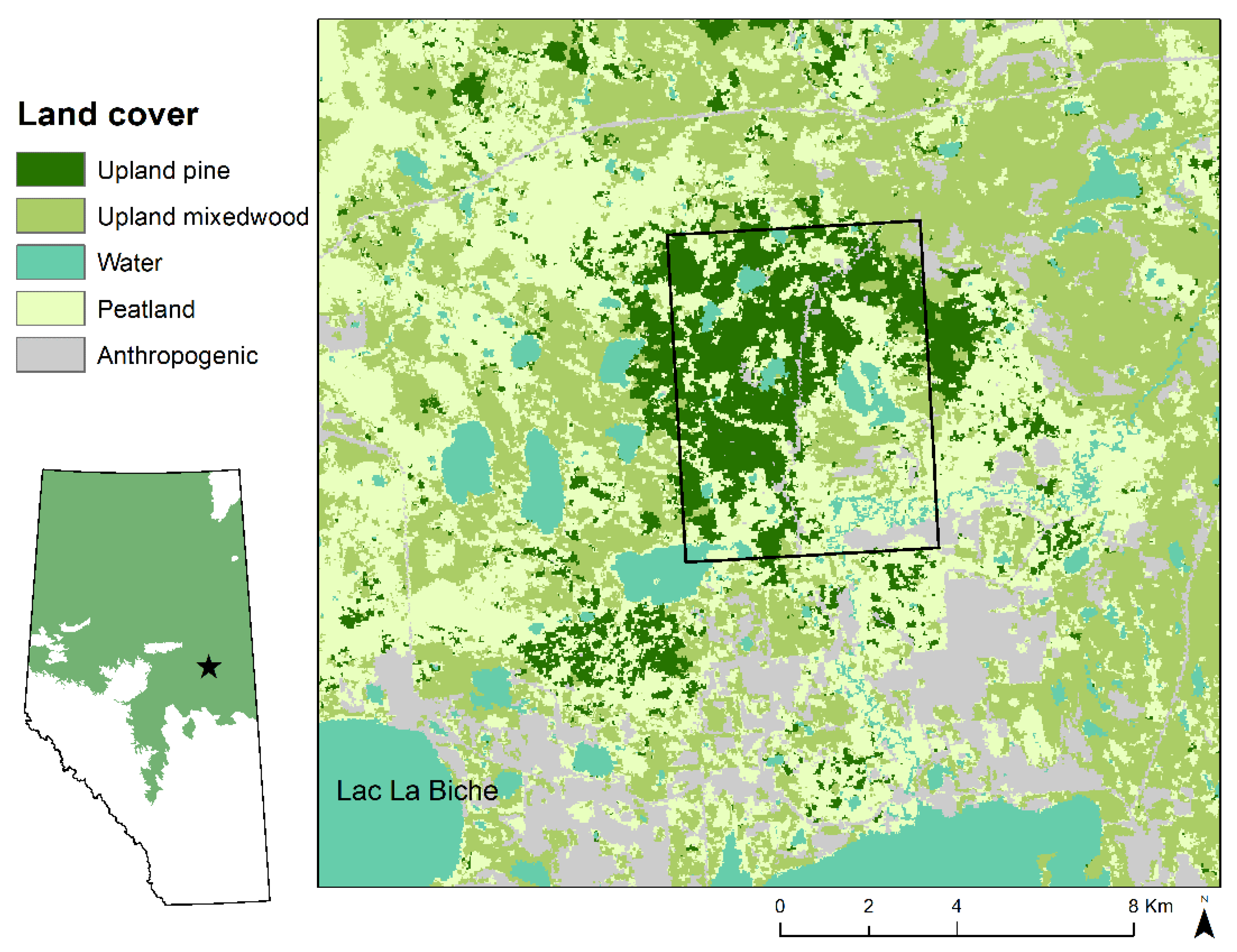
2.1. Study Area

We estimated lichen cover for 15 mature, jack pine dominated forest stands located in the dry mixedwood subregion of the boreal forest within the south boreal transition zone 25 km north of Lac La Biche, Alberta, Canada (Figure 1). The dry mixedwood is characterized by upland aspen (Populus tremuloides) forests, open jack pine (Pinus banksiana) stands with lichen-dominated understory (Figure 2a), and lowland fens [19]. The area is classified as mature forest, and has not been disturbed by fire in at least 80 years [20]. Lichens are uncommon in aspen and mixedwood stands due to high levels of shading and competition with vascular plants, thus these habitat types were excluded from the study. Since lowland fens are characterized by having a high and fluctuating water table that results in conditions too wet for abundant ground lichen growth, we also excluded lowlands from our study. That leaves mature jack pine stands with abundant mats of Cladonia lichens, sparse ground vegetation (consisting predominantly of Arctostaphylos uva-ursi, Vaccinium myrtilloides, and Maianthemum canadense), and feather-mosses. Reindeer lichen species in the area consists of Cladonia arbuscula ssp. mitis, Cladonia uncialis, Cladonia rangerifina, Cladonia amaurocrea, Cladonia stellaris, and Cladonia stygia.

2.2. Remote Sensing Predictor Variables

The Government of Alberta has acquired ALS data for over 33 million hectares of forested regions in the province, with data used for this study collected on 11 May 2009 [22]. Pulse density for these data ranged from 1 to 4 returns per m² with a scan angle of <25° from nadir and vertical accuracy of no greater than 30 cm root mean square error [23]. Bare-Earth digital elevation models (DEM) derived from these data were subtracted from the ALS-derived digital surface model (DSM) to derive tree heights. A suite of forest canopy raster metrics were developed at 30 m resolution using FUSION software [24] by the Government of Alberta and provided to us for use. Although these data were collected earlier than our study, the study area has not experienced any major disturbances since collection and tree growth in these unproductive sites is slow. Due to the mature status of these forest stands, metrics derived from ALS will not therefore have changed substantially.

While stand age is an important factor in lichen abundance due to its slow growth, our study area contained little variation in stand age (>90 years), and thus tree heights were similar. We therefore excluded ALS tree height variables and instead focused on horizontal (canopy) cover since light is a more important predictor of lichen abundance [1]. Specifically, we defined canopy cover as the fraction of first ALS returns over 1.37 m in height. In upland habitats, lichen preferentially grows in dry, sandy soils, so surficial geology data [25] related to the presence of sandy substrates (here eolian deposits) was considered but subsequently removed since it did not vary across our study plots. As lichen prefers drier conditions and can be limited by a high water table, depth to water table (DWT) was included as a potential predictor of lichen abundance [26]. DWT was derived from ALS data, using predicted stream lines as a reference [26]. All predictor variables were resampled to 2.8 m resolution using the bilinear interpolation method to match spectral data.

KOMPSAT-3 [27] is an optical high-resolution (280 cm) satellite with 1.4 day revisit time. Multispectral imagery is collected in 4 bands: red, green, blue, and near-infrared. For spectral remotely sensed data, we used imagery from KOMPSAT-3 [27] ortho-rectified with imagery from Pleiades satellite [28]. Based on cloud-free coverage of our study area, imagery used in our study was collected on 4 June 2016. Despite an approximate 1 year discrepancy between the date of image collection and date of field sampling, the degree of lichen abundance may be expected to be unchanged over this time, as lichen is slow-growing and no observable disturbance occurred between image collection and field sampling dates. Imagery was reprojected in Alberta 10TM projection for further analysis. See

Table 1. Predictor variable values for low, moderate, and high canopy plots. Minimum, median, maximum, and mean values (including standard error (SE)) are provided for airborne laser scanning (ALS)-derived canopy cover, KOMPSAT-3 blue band, and depth to water table (DWT).

Predictor Variable	Minimum	Median	Maximum	Mean (SE)
Canopy cover < 25%
ALS-derived canopy cover (%)	6	25	64	26.92 (3.31)
KOMPSAT-3 blue band (reflectance value)	0.30	0.60	1.00	0.60 (0.03)
DWT (m)	2	5	9	5.08 (0.40)
Canopy cover 25–50%
ALS-derived canopy cover (%)	13	53	59	48.96 (2.14)
KOMPSAT-3 blue band (reflectance value)	0.07	0.31	0.73	0.34 (0.04)
DWT (m)	0	3	10	3.92 (0.62)
Canopy cover > 50%
ALS-derived canopy cover (%)	57	68	82	68.08 (1.54)
KOMPSAT-3 blue band (reflectance value)	0.00	0.13	0.25	0.13 (0.01)
DWT (m)	0	1	4	1.68 (0.26)

for a summary of predictor variable values.

2.3. Sample Plot Selection

Jack pine stands were selected for sampling in ArcMap [29] using the enhanced wetland classification layer from Ducks Unlimited [21]. Specifically, plots were stratified by canopy cover using ALS data on the fraction of points over 1.37 m height (30 m cell size) and dividing the region into low (<25%), moderate (25–50%), and high (>50%) canopy cover, with 5 replicate plots selected in each canopy cover strata for a total 15 plots. Sites with low canopy cover made up 20% of the study area (342.09 ha), moderate canopy cover made up 34% of the study area (594.36 ha), and high canopy cover made up 46% (799.56 ha) of the study area.

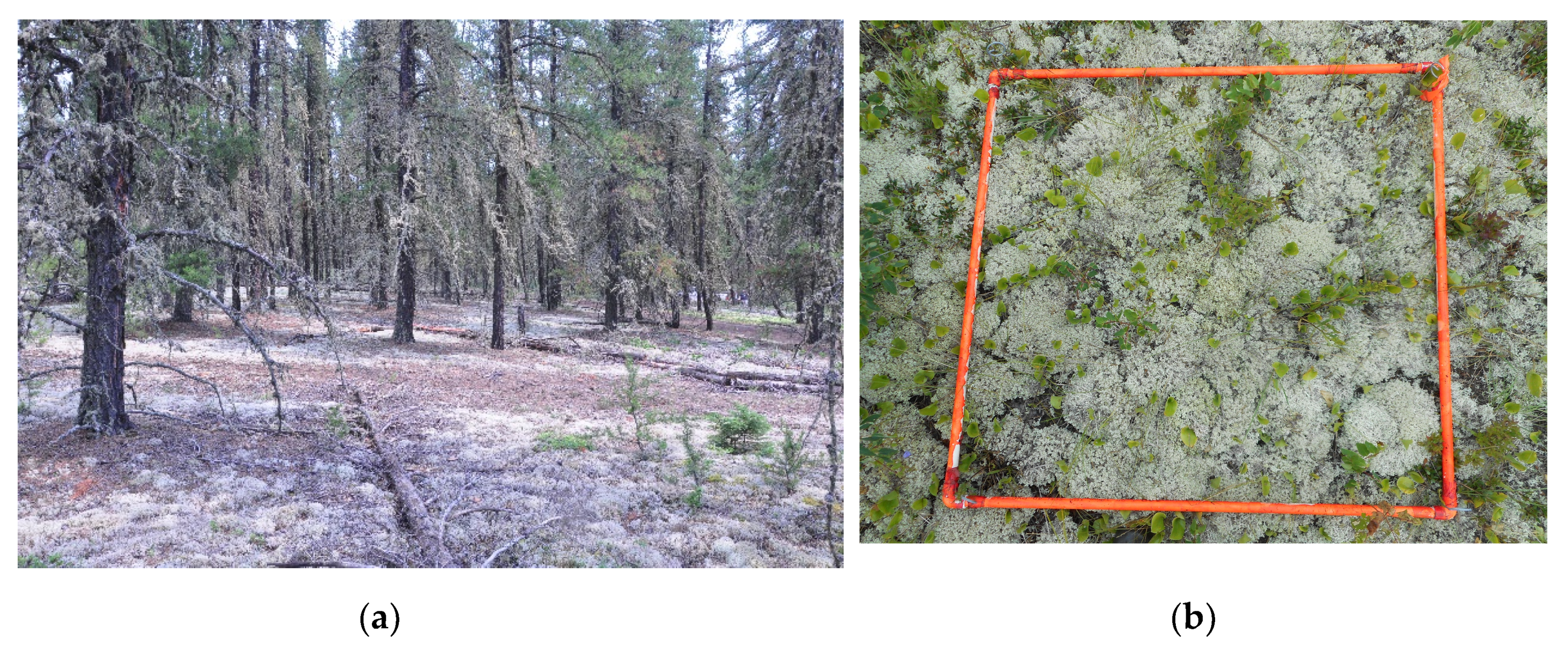
2.4. Field Measurements of Cover and Biomass

Sample plots were 20 m² in size, with five 1 m² quadrats located in the centre and corners of each plot (75 total subplots, see Figure 2b example) and surveyed in June 2017. Within each plot, we visually estimated percent cover (within the nearest 5th percentile) and measured average height (in cm) of each reindeer lichen species, as well as cover of other lichen species. Ground cover was estimated for other items (within the nearest 5th percentile), including vascular plants, litter, bare ground, and downed woody material. We measured canopy cover above each quadrat using a spherical densiometer. For a subsample of plots (3 plots in low canopy cover, 3 plots in medium canopy cover, and 3 plots in high canopy cover), we harvested all lichen within each 1 m² quadrat. In the lab, we hand sorted harvested lichen to remove twigs, leaves, and other debris, and then oven dried samples at 70 °C for 24 h at which point we weighed each sample (by species) to determine dry biomass.

2.5. Allometric Model of Lichen Cover and Biomass

For harvested plots, g/m² biomass per plot (20 m² plot) was averaged from all quadrats and compared to lichen cover to estimate the relationship between lichen cover and biomass (i.e., the allometric relationship) using linear regression. Due to the inability of satellite imagery to determine lichen species, as well as low sample size for some species, all species data were pooled when estimating the cover to biomass relationship. Allometric equations derived from this model were then applied to the remaining plots to predict lichen biomass (g/m²) for all plots. Initially both cover and height of lichens were considered in the allometric model, but here we only report on the relationships with cover as there was little support for including height in these equations, potentially due to the similarity of stand age across study plots (all pine stands > 90 years old with older patches of lichen).

2.6. Statistical Modelling

Tree height metrics and the fraction of returns between 0.15 and 1.37 m showed no significant relationship with lichen biomass (p = 0.43 and p = 0.32, respectively) and were removed from further model selection. Since lichens are known to show high reflectance in the blue wavelength, band 3 of the KOMPSAT imagery was used in all models, while bands 1 and 2 that were correlated (r > 0.7) with band 3 were excluded. Non-linear quadratic functions were also tested for each variable, as well as interaction terms between all variables.

To compare remotely sensed variables, we developed 8 candidate models that represented different a priori hypotheses. Each remotely sensed variable was considered as an independent predictor, and they were also used in combination with band 3 and canopy cover, as these variables were anticipated to be the most related to lichen biomass. We also considered the interaction between each variable and band 3 (see

Table 2. Name and structure of candidate models used to predict lichen biomass. Covariates within the same model have a Pearson’s correlation coefficient > |0.7|. DWT refers to the depth to water table, Blue refers to blue spectral data, and canopy refers to canopy cover.

Model Name	Model Structure
Blue spectrum	Biomass ~ band 3
Canopy cover	Biomass ~ canopy
Depth-to-water (DWT)	biomass ~ logDWT
Blue + Canopy cover	biomass ~ band 3 + canopy
Blue + DWT	biomass ~ band 3 + log DWT
Blue × Canopy cover	biomass ~ band 3 + canopy + band3 × canopy
Blue × DWT Null	biomass ~ band 3 + logDWT + band3 × logDWT biomass ~ 1 + plot random effect

). Additionally, we tested a null model to assess how much more the final model was supported over a simple null model that effectively predicted the same lichen biomass (mean value) across all plots.

Values for each remotely sensed variable were acquired for all quadrat locations and fit with a series of generalized linear mixed-effect models, using the glmmTMB package in R [30].. All models used a Gaussian family, and plot ID was used as a random effect to account for nested observations (multiple quadrats within the plot). Akaike’s information criterion (AIC) was used to evaluate model selection (support among models). Assessment of overall model fit was determined using pseudo-R-squared for generalized mixed-effects models in the MuMIn package in R [31]. The most supported model from AIC was then predicted across the study area using Spatial Analyst Map Algebra tool in ArcMap using model coefficients and spatial layers [29]. Other light-coloured objects, such as sand roads or senesced vegetation in riparian areas, were masked in map predictions.

3. Results

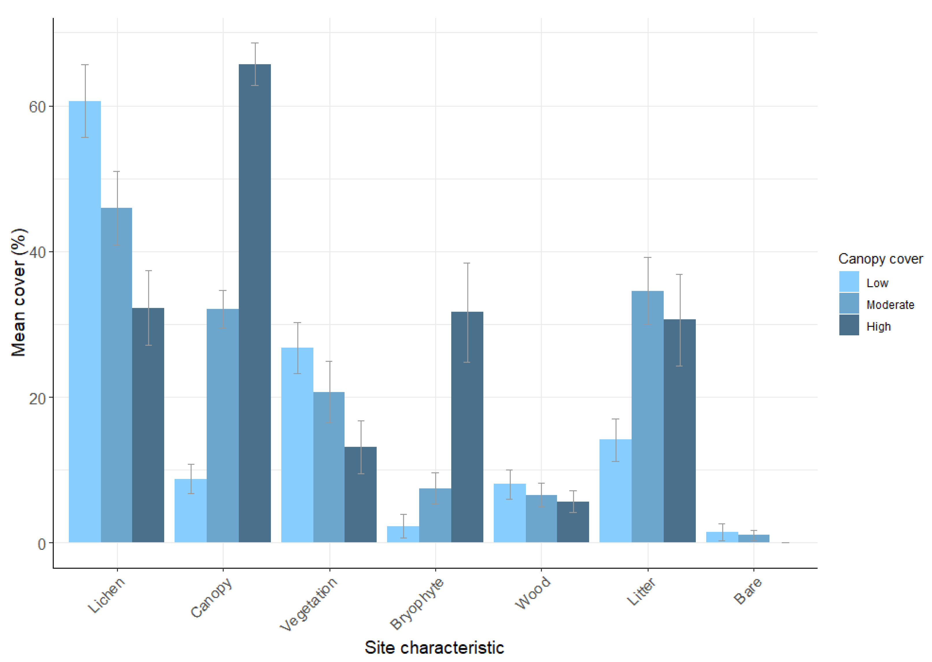
3.1. Plot Characteristics

Spherical densiometer measurements of canopy cover in study plots for the low canopy strata averaged 8.8% (SE = 2.0), 32.1% (SE = 2.5) for the moderate canopy strata, and 65.7% (SE = 2.9) for the high canopy strata. Lichen abundance was lowest within the high canopy cover strata averaging 32.3% cover (SE = 5.1) and 98.96 g/m² of dry biomass. Lichen abundance in moderate canopy strata averaged 45.9% (SE = 5.1) cover and 140.93 g/m² of dry biomass. Lichen abundance in low canopy strata supported approximately double the amount of lichen as in plots with high canopy cover, averaging 60.6% (SE = 5.0) cover and 186.27 g/m² of dry biomass. Other ground cover, including vegetation, bryophyte, litter, and downed woody material varied from 0% to 90% cover. See Figure 3 for summary statistics of plot and stand characteristics.

The linear relationship between lichen cover and biomass was y = 7.3478x (p < 0.001, R² = 0.82; Figure 4). For every 1% increase in lichen cover, biomass increased by 7.3478 g/m². Scatter within the observations may be related to species of lichen with each plot. For example, observations that show low lichen cover but high biomass tended to have a higher abundance of Cladonia uncialis, a densely matted, robust species. Observations with high lichen cover but low biomass tended to have a higher abundance of Cladonia arbuscula sp. mitis, which tends to mat more sparsely and show more extensive branching. Due to the inability of optical imagery to distinguish between species, this data was not included in further analysis.

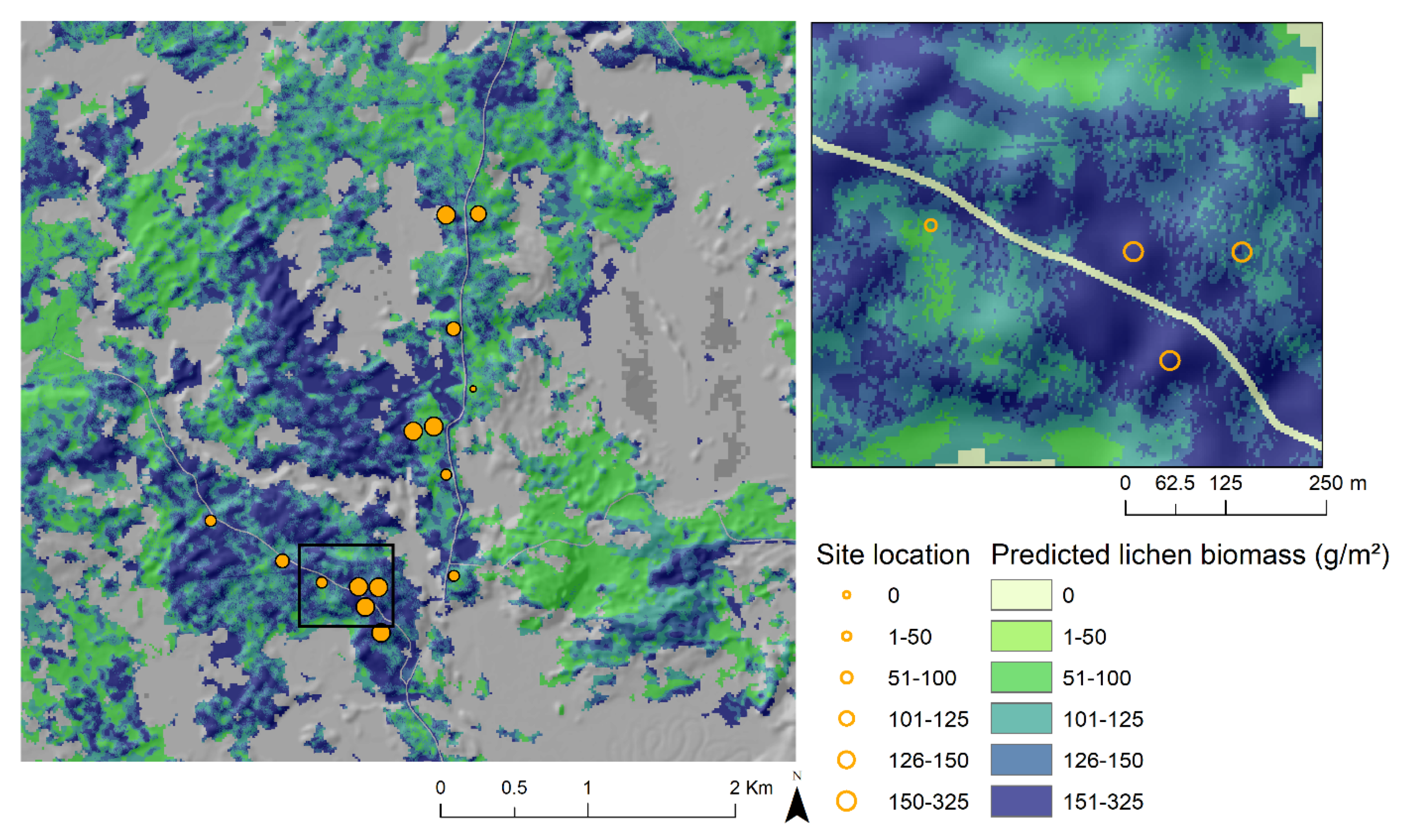
3.2. Model Selection

Canopy cover (ALS returns above 1.37) was significantly related lichen biomass (p = 0.001), as was DWT (p < 0.001). Band 1 (red band), band 2 (green band), and band 3 (blue band) were all correlated to lichen biomass (p = 0.012, p = 0.007, and p = 0.017, respectively), however high correlation was observed between bands (Pearson’s correlation coefficient > |0.7|).

Overall, the most supported model included either canopy cover (i.e., canopy) or band 3 and canopy cover (i.e., band 3 and canopy) combined (Akaike weights w_i = 0.433 and 0.276, respectively;

Table 3. Ranking of model support for a series of models predicting ground lichen biomass (g/m²) in jack pine stands based on remotely sensed data using Akaike’s information criterion (AIC). Model name, parameter number, change in AIC, and Akaike weights are provided. Blue + canopy cover was chosen as the model of best fit. Band 3 is derived from satellite imagery (KOMPSAT), while canopy cover is derived from Airborne laser scanning (ALS) first returns above 1.37 m. DWT refers to the depth to water table.

Model	K	AIC	∆AIC	wi
Canopy cover	2	867.3	0.0	0.433
Blue + Canopy cover	3	868.2	0.9	0.276
Blue + DWT	3	869.9	2.6	0.118
Blue spectrum	2	870.6	3.3	0.083
Blue × Canopy cover	4	872.0	4.7	0.041
Blue × DWT	4	873.5	6.2	0.020
Null	2	873.5	6.2	0.020
DWT	2	875.1	7.8	0.009

). The model that included both spectral and structural variables was within ∆AIC < 2.0 (∆AIC = 0.9) and given that the aim of this study was to assess relationships between spectral satellite data and ALS-derived stand structure data on lichen biomass, we chose the model including band 3 and canopy cover (∆AIC = 0.9) for further reporting. When considering individual predictors, there was no support for including DWT as it was shown to be the poorest predictor of lichen biomass. The canopy variable alone was more supported (more than 5-fold) than that of the spectral data alone (∆AIC = 3.3).

The model of best fit (R² c = 0.35) demonstrated a positive relationship between band 3 (blue) and lichen biomass (

Table 4. Model parameters relating remote sensed variables to lichen biomass within jack pine forests in central Alberta, Canada. Variable name, beta-values (β), standardized beta (Beta), standard error (Std. Error), z value (z), and significance values (p) are provided. Band 3 refers to blue spectral values from KOMPSAT-3 imagery, while LiDAR refers to canopy cover derived from ALS.

Variable	β Value	Beta	Std. Error	z	p
Intercept	156.70		67.53	2.32	0.020
band 3 (blue)	0.03	0.15	0.03	1.06	0.290
Lidar (canopy cover)	−1.34	−0.32	0.64	−2.1	0.035

) where an increase in band 3 reflectance is related to higher lichen biomass. Specifically, for each one unit increase in spectral value of band 3, lichen biomass increased by 0.03 g/m². In contrast, a negative relationship was observed between lichen biomass and canopy cover (Table 4). Specifically, for every 1 unit increase in percent canopy cover, lichen biomass decreased by 1.34 g/m². Standardized coefficients illustrated a stronger effect of canopy cover over that of spectral data with canopy cover being 2-fold greater in absolute effect (Table 4). We tested our final model with lichen cover as the response variable and found similar results to that of lichen biomass (band 3: β = 0.01, canopy cover: β = −0.38), however a lower overall fit (R² = 0.20).

As a demonstration of the developed model, we predicted lichen biomass for our study area (Figure 5). A clear pattern of lichen abundance was observed, with areas of predicted high abundance occurring in areas where forest canopy is open and blue spectral reflectance is high.

4. Discussion

The boreal forest consists of a complex structure composed of overstory trees and understory vegetation. The abundance, diversity, and structure of the understory is linked to the structure of the overstory, as changes in light availability from the canopy affect the productivity of the understory [32]. In general, the link between overstory structure and understory composition has been largely understudied in the boreal forest, with studies focusing primarily on tree characteristics or understory characteristics in isolation [33]. Additionally, studies that rely on remote sensing products, which cannot map the understory through the canopy, often rely on overstory measurements as a metric of understory characteristics, however without simultaneous ground truthing and overstory measurements, it is difficult to associate understory patterns with exact overstory structure [33]. Majasalmi and Rautiainen [33] found that understory characteristics varied with canopy cover metrics, and that canopy cover was a better indicator of understory structure than other forest metrics. In lichen dominated understories in particularly, lichen abundance has been shown to be closely tied to canopy cover [34]. The patchiness of lichen distribution can therefore be attributed to patchiness in canopy cover [34], and can be deduced by overstory metrics derived from remote sensing.

We mapped lichen biomass for a dry, upland jack pine stand in the south boreal transition zone using high-resolution spatial imagery and ALS data. By applying spatial data from KOMPSAT imagery and structural data from ALS to field measurements of lichen biomass, we identified site characteristics, spectral bands, and forest stand characteristics that best related to lichen abundance. Overall, we found that canopy cover and the blue spectral band were the most important predictors of lichen biomass with canopy cover being a better single predictor of lichen abundance than spectral data. Lichen biomass was positively related to areas of open canopy. Lichens require sufficient amounts of sunlight and water (precipitation) to photosynthesize [3], which they can more readily get under open canopy conditions. Forests with low canopy cover contained almost double the biomass of high canopy cover, suggesting that as the canopy cover increases, shade tolerant bryophytes outcompete lichens [1]. Indeed, we observed a 10-fold increase in bryophyte cover between plots with low canopy cover and plots with high canopy cover (Table 1). However, due to the small area of this study (4200 ha) and the relatively homogenous stands of open pine, as well as the overall low abundance and diversity of vascular and non-vascular plants, we did not consider abundance of other plants and bryophytes within these models, but instead focused on the use of remotely sensed information.

For spectral information, we found that the blue spectral band of KOMPSAT imagery was the best predictor of lichen biomass (p = 0.012). There was a positive relationship between blue spectral values and lichen biomass (β = 0.03), suggesting that in areas where blue band reflectance is high, lichen biomass is also high. While the blue spectrum can be sensitive to atmospheric scattering, ground lichens tend to exhibit backward scatter, differentiating them from surrounding vegetation that tends to exhibit forward scatter [35]. There are, however, some limitations to using spectral data alone in mapping lichen abundance. For example, other light coloured objects in the imagery, such as sandy roads and senesced vegetation along riparian zones also have high reflectance in the blue band. We masked these features to exclude them from the analysis.

There are several factors that should be taken into consideration when applying our approach to a larger spatial scale. For example, lichens can occur in low to moderate abundance in peatland habitats [2]. Although peatlands were present in our study area, they were excluded due to low or no lichen abundance. Subsequent studies should incorporate both peatlands and upland areas across a larger region with different stand ages. Under those conditions the value of other variables in predicting lichen abundance, including DWT, may be quite different than observed for mature open jack pine stands. Additionally, due to the importance of fire as a natural disturbance in the boreal, the effect of fire intensity, fire severity, and regeneration of tree stands on lichen regeneration and growth need to be considered. The presence of fire greatly affects lichen abundance and available winter forage for caribou. Due to the homogeneity and maturity of our study area, fire severity and time since fire were not included. Future work should include lichen biomass measurements at various stand ages post-fire to assess the ability of spectral band data to detect lichen recovery over time. Although lichen cover has been shown to be useful in predicting lichen biomass, lichen height also contributes to its biomass, can be used to estimate lichen growth rate [36], and may indicate changes to lichen biomass that may not be accounted for by cover alone. Average height of lichens in our study did not contribute significantly to estimates of lichen biomass and was excluded, but is likely to be important elsewhere, especially for younger stands. Additional work on this subject should measure average lichen height across a range of plots that vary in lichen abundance in order to establish more robust relationships between lichen height and biomass.

Limitations in acquisition will place limitations on the use of ALS-derived canopy cover as a predictor of lichen abundance. Our study area had not experienced significant disturbance since ALS data was acquired in 2009, therefore we can reasonably estimate lichen biomass using this metric. However, in other areas where disturbance occurs more frequently, canopy cover derived from ALS may not accurately represent current canopy conditions. In studies without up to date ALS data, there is need for additional field measurements of canopy cover.

Our a priori models showed little variation in AIC values, suggesting that the predictive power of our models did not differ greatly. Due to the homogeneity (i.e., little variation in ecosite type, stand age, and lichen abundance) of our study area, we expect that our predictor variables did not differ greatly enough to show high variation in AIC values. In more heterogeneous areas, larger differences between models may be expected.

The use of high-resolution KOMPSAT imagery demonstrates that fine spatial scale imagery can be useful for predicting lichen abundance, since even small canopy gaps can significantly increase lichen abundance. Previous studies using spectral data to predict ground lichens relied on coarser resolution Landsat or SPOT imagery [12,13,17] at resolutions of 30 m or 10 m, respectively. While these studies have shown success mapping lichen abundance at broad spatial scales, the use of 280 cm KOMPSAT can be used to accurately estimate patterns in lichen biomass that may not be evident at broader scales. The predictive power of our model (R² c = 0.35) may be impacted by the early date of KOMPSAT data collection (4 June 2016). Image collection at this stage of the growing season may be too early to fully capture peak vegetation cover, thereby reducing the overall contrast between green vegetation and light-coloured lichens. Given the homogeneity of our study area, our model could have been strengthened further by considering greater environmental variation, including topography, ecosite type, and changes in soil type. This study area was selected due to the known presence and abundance of terricolous lichens with the objective of testing field methodology and predictive value of available high resolution, multi-spectral imagery. Our model of best fit was reasonable in estimating general patterns in lichen abundance based on variation in canopy cover and spectral data. As we demonstrated in our map of lichen abundance, fairly simple models based on ALS and optical satellite data can be used to map spatial variations in lichen abundance. We provide our raw data as an Appendix (

Table A1. Raw field data for surveyed plots. Quadrat location, lichen cover (%), lichen biomass (g/m²), canopy cover derived from ALS (%), and blue band spectral values are provided. Locations are collected in NAD83.

Plot	Quadrat	Easting	Northing	Lichen Cover (%)	Lichen Biomass (g/m2)	ALS-Derived Canopy Cover (%)	Band 3 (Blue)
L1	L1-C	435310.41	6093434.95	84	258.03	7	1853
L1	L1-NE	435319.23	6093443.17	2	6.14	7	2044
L1	L1-SE	435319.28	6093424.69	74	227.31	7	2405
L1	L1-SW	435300.41	6093425.63	62	190.45	25	1977
L1	L1-NW	435302.57	6093446.64	69	211.95	18	1610
L2	L2-C	435272.78	6093572.72	55	168.95	15	1926
L2	L2-NE	435280.45	6093581.18	80	245.74	15	2058
L2	L2-SE	435281.30	6093560.35	87	267.25	32	2019
L2	L2-SW	435260.19	6093560.88	30	92.15	32	2189
L2	L2-NW	435263.24	6093581.09	92	282.61	15	1953
L3	L3-C	436011.89	6096061.35	45	138.23	39	1810
L3	L3-NE	436023.26	6096068.65	52	159.73	39	1848
L3	L3-SE	436021.27	6096050.76	36	110.58	39	1604
L3	L3-SW	436000.76	6096052.05	80	245.74	39	1881
L3	L3-NW	436002.63	6096070.84	34	104.44	39	1511
L4	L4-C	435702.91	6094608.81	87	267.25	37	1527
L4	L4-NE	435713.12	6094620.01	35	107.51	64	2099
L4	L4-SE	435714.29	6094598.74	54	165.88	64	2630
L4	L4-SW	435694.39	6094603.25	25	76.80	37	1446
L4	L4-NW	435695.17	6094622.39	95	291.82	37	1986
L5	L5-C	435407.70	6093253.91	98	301.04	6	2266
L5	L5-NE	435416.70	6093265.36	52	159.73	24	1944
L5	L5-SE	435417.40	6093247.32	46	141.30	6	2303
L5	L5-SW	435396.90	6093245.72	72	221.17	6	2333
L5	L5-NW	435397.91	6093267.91	70	215.03	24	1674
M1	M1-C	435407.39	6093564.43	75	230.39	53	1639
M1	M1-NE	435418.35	6093574.51	82	251.89	53	1537
M1	M1-SE	435417.98	6093553.59	57	175.09	55	1451
M1	M1-SW	435397.47	6093556.23	90	276.46	56	1465
M1	M1-NW	435398.64	6093575.02	72	221.17	47	1644
M2	M2-C	434766.11	6093777.52	36	110.58	28	2158
M2	M2-NE	434772.69	6093790.00	47	144.37	46	1190
M2	M2-SE	434773.59	6093768.06	45	138.23	28	1300
M2	M2-SW	434755.49	6093773.33	20	61.44	43	1755
M2	M2-NW	434757.06	6093788.89	52	159.73	13	1357
M3	M3-C	434295.61	6094080.33	4	12.29	48	1292
M3	M3-NE	434307.67	6094090.84	10	30.72	48	1491
M3	M3-SE	434304.34	6094073.20	41	125.94	53	2176
M3	M3-SW	434285.74	6094074.92	55	168.95	55	1233
M3	M3-NW	434286.62	6094091.37	40	122.87	45	2151
M4	M4-C	436015.54	6095286.12	42	129.02	59	1134
M4	M4-NE	436024.67	6095291.11	7	21.50	53	1403
M4	M4-SE	436024.32	6095271.09	32	98.30	53	1374
M4	M4-SW	436002.78	6095271.95	32	98.30	59	1567
M4	M4-NW	436003.72	6095293.42	75	230.39	59	1822
M5	M5-C	436230.31	6096055.12	87	267.25	54	1261
M5	M5-NE	436239.56	6096066.23	55	168.95	54	1369
M5	M5-SE	436239.25	6096049.20	55	168.95	54	1595
M5	M5-SW	436218.95	6096047.49	30	92.15	54	1053
M5	M5-NW	436220.02	6096064.28	6	18.43	54	1041
H1	H1-C	435023.08	6093619.85	30	92.15	58	1207
H1	H1-NE	435032.45	6093630.07	17	52.22	58	1148
H1	H1-SE	435032.31	6093607.37	50	153.59	60	1125
H1	H1-SW	435013.39	6093604.19	42	129.02	77	1196
H1	H1-NW	435014.79	6093630.44	7	21.50	67	1332
H2	H2-C	435922.83	6093611.45	0	0.00	60	1163
H2	H2-NE	435932.76	6093616.31	17	52.22	60	970
H2	H2-SE	435932.05	6093598.18	8	24.57	60	1359
H2	H2-SW	435911.61	6093601.26	0	0.00	67	1212
H2	H2-NW	435912.07	6093619.95	50	153.59	67	1249
H3	H3-C	435911.01	6094300.87	22	67.58	74	1199
H3	H3-NE	435922.42	6094306.72	17	52.22	74	1262
H3	H3-SE	435920.04	6094288.17	8	24.57	74	1058
H3	H3-SW	435899.31	6094288.35	17	52.22	57	1296
H3	H3-NW	435900.35	6094307.48	67	205.81	57	1203
H4	H4-C	436125.92	6094872.09	27	82.94	76	928
H4	H4-NE	436135.71	6094881.41	22	67.58	76	1016
H4	H4-SE	436138.37	6094861.67	2	6.14	82	1132
H4	H4-SW	436117.24	6094859.97	0	0.00	82	1037
H4	H5-NW	436118.28	6094879.66	24	73.72	76	986
H5	H5-C	435844.78	6094631.70	80	245.74	68	1130
H5	H5-NE	435856.22	6094639.66	42	129.02	68	1145
H5	H5-SE	435855.30	6094624.65	60	184.31	68	1059
H5	H5-SW	435838.90	6094622.99	45	138.23	68	1300
H5	H5-NW	435835.54	6094638.73	87	267.25	68	1001

) to foster development of models applicable to larger areas. The benefit of our approach is that it can easily be reproduced in other regions with more variation in ecosystem properties.

5. Conclusions

In this study, we developed and applied an approach to quantify lichen cover and biomass based on field data, airborne laser scanning, and high spatial resolution optical data, using a pine dominated site in boreal Canada as a case study area. We used field measurements to establish an allometric relationship between lichen cover and biomass for jack pine stands to facilitate easier estimation of biomass. We found that blue spectral data from KOMPSAT and canopy cover from aerial ALS best predicted lichen biomass. The overall fit of this model (R² c = 0.35) suggests these two remote sensing variables can reasonably estimate patterns in lichen abundance. Our approach to mapping lichen abundance suggests that high resolution remotely sensed data could be used to map spatial variations in lichen abundance.

References

1. Vitt, D.H.; Finnegan, L.; House, M. Terrestrial bryophyte and lichen responses to canopy opening in pine-moss-lichen forests. Forests 2019, 10, 233. [Google Scholar] [CrossRef] [Green Version]
2. Dunford, J.S.; McLoughlin, P.D.; Dalerum, F.; Boutin, S. Lichen abundance in the peatlands of northern Alberta: Implications for boreal caribou. Ecoscience 2007, 13, 469–474. [Google Scholar] [CrossRef]
3. Hale, M. The Biology of Lichens, 2nd ed.; Edward Arnold Publishers Ltd.: London, UK, 1974. [Google Scholar]
4. Environment Canada. National Recovery Strategy for Woodland Caribou (Rangifer tarandus caribou), Boreal Population, in Canada; Environment Canada: Ottawa, ON, Canada, 2012; ISBN 9781100207698.
5. COSEWIC. Assessment and Update Status Report on the Woodland Caribou; Committee on the Status of Endangered Wildlife of Canada: Ottawa, ON, Canada, 2002. [Google Scholar]
6. McLoughlin, P.D.; Dzus, E.; Wynes, B.; Boutin, S. Declines in Populations of Woodland Caribou. J. Artic. 2019, 67, 755–761. [Google Scholar] [CrossRef]
7. Dickie, M.; Serrouya, R.; McNay, R.S.; Boutin, S. Faster and farther: Wolf movement on linear features and implications for hunting behaviour. J. Appl. Ecol. 2017, 54, 253–263. [Google Scholar] [CrossRef]
8. Wotton, B.M.; Flannigan, M.D.; Marshall, G.A. Potential climate change impacts on fire intensity and key wildfire suppression thresholds in Canada. Environ. Res. Lett. 2017, 12, 9. [Google Scholar] [CrossRef]
9. Klein, D.R. Fire, Lichens, and Caribou. J. Range Manag. 2007, 35, 390. [Google Scholar] [CrossRef]
10. Metsaranta, J.M. Assessing the length of the post-disturbance recovery period for woodland caribou habitat after fire and logging in west-central Manitoba. Rangifer 2007, 27, 103. [Google Scholar] [CrossRef] [Green Version]
11. Petzold, D.E.; Goward, S.N. Reflectance spectra of subarctic lichens. Remote Sens. Environ. 1988, 24, 481–492. [Google Scholar] [CrossRef]
12. Gilichinsky, M.; Sandström, P.; Reese, H.; Kivinen, S.; Moen, J.; Nilsson, M. Mapping ground lichens using forest inventory and optical satellite data. Int. J. Remote Sens. 2011, 32, 455–472. [Google Scholar] [CrossRef]
13. Nelson, P.R.; Roland, C.; Macander, M.J.; McCune, B. Detecting continuous lichen abundance for mapping winter caribou forage at landscape spatial scales. Remote Sens. Environ. 2013, 137, 43–54. [Google Scholar] [CrossRef]
14. Rosso, A.; Neitlich, P.; Smith, R.J. Non-destructive lichen biomass estimation in northwestern Alaska: A comparison of methods. PLoS ONE 2014, 9, e103739. [Google Scholar] [CrossRef]
15. Lim, K.; Treitz, P.; Wulder, M.; St-Ongé, B.; Flood, M. LiDAR remote sensing of forest structure. Prog. Phys. Geogr. 2003, 27, 88–106. [Google Scholar] [CrossRef] [Green Version]
16. Falldorf, T.; Strand, O.; Panzacchi, M.; Tømmervik, H. Estimating lichen volume and reindeer winter pasture quality from Landsat imagery. Remote Sens. Environ. 2014, 140, 573–579. [Google Scholar] [CrossRef] [Green Version]
17. Kennedy, B.; Pouliot, D.; Manseau, M.; Fraser, R.; Duffe, J.; Pasher, J.; Chen, W.; Olthof, I. Assessment of Landsat-based terricolous macrolichen cover retrieval and change analysis over caribou ranges in northern Canada and Alaska. Remote Sens. Environ. 2020, 240, 111694. [Google Scholar] [CrossRef]
18. Konkolics, S.M. A Burning Question: The Spatial Response of Woodland Caribou to Wildfire in Northeastern Alberta. Master’s Thesis, Department of Biological Sciences, University of Alberta, Edmonton, AB, Canada, 2019. [Google Scholar]
19. Downing, D.J.; Pettapiece, W.W. Natural Regions and Subregions of Alberta; Government of Albeta: Stony Plain, AB, Canada, 2006; ISBN 0778545725.
20. Alberta Wildfire. Historical Wildfire Perimeter Data: 1931–2017. Available online: http://wildfire.alberta.ca/resources/historical-data/spatial-wildfire-data.aspx (accessed on 1 April 2017).
21. Ducks Unlimited. Enhanced Wetland Classifcation Layer; Ducks Unlimited: Edmonton, AB, Canada, 2011. [Google Scholar]
22. Guo, X.; Coops, N.C.; Tompalski, P.; Nielsen, S.E.; Bater, C.W.; John Stadt, J. Regional mapping of vegetation structure for biodiversity monitoring using airborne lidar data. Ecol. Inform. 2017, 38, 50–61. [Google Scholar] [CrossRef]
23. Alberta Environment and Sustainable Resource Develeopment. General Specifications for Acquisition of LiDAR Data; Environment and Sustainable Resource Development: Edmonton, AB, Canada, 2013. [Google Scholar]
24. McGaughey, R.J. FUSION/LDV: Software for LIDAR Data Analysis and Visualization; US Department of Agriculture Forest Service Pacific Northwest Research Station: Seattle, WA, USA, 2014.
25. Alberta Geological Survey. Surficial Geology of Alberta, Generalized Digital Mosaic (DIG 2013-0002). Available online: https://geology-ags-aer.opendata.arcgis.com/datasets/surficial-geology-of-alberta-generalized-digital-mosaic-dig-2013-0002 (accessed on 1 April 2017).
26. Alberta Agriculture and Forestry. Wet Areas Mapping. Available online: https://geodiscover.alberta.ca/geoportal/rest/metadata/item/2ef5a9d1b2154067bc1af0160499ef3c/html (accessed on 1 April 2017).
27. Korean Aerospace Research Institute. KOMPSAT-3 Data; Korean Aerospace Research Institute: Daejeon, Korea, 2016.
28. French Space Agency. Pleidates 1 Satellite Data; French Space Agency: Paris, French, 2016.
29. ESRI. ArcGIS Desktop: Release 10; Environmental Systems Research Institute: Redlands, CA, USA, 2011. [Google Scholar]
30. Brooks, M.E.; Kristensen, K.; van Benthem, K.J.; Magnusson, A.; Berg, C.W.; Nielsen, A.; Skaug, H.J.; Maechler, M.; Bolker, B.M. glmmTMB balances speed and flexibility among packages for zero-inflated generalized linear mixed modeling. R J. 2017, 9, 378–400. [Google Scholar] [CrossRef] [Green Version]
31. Barton, K. Mu-MIn: Multi-model Inference. 2009. Available online: http://R-Forge.R-project.org/projects/mumin/ (accessed on 1 September 2017).
32. Barbier, S.; Gosselin, F.; Balandier, P. Influence of tree species on understory vegetation diversity and mechanisms involved-A critical review for temperate and boreal forests. For. Ecol. Manag. 2008, 254, 1–15. [Google Scholar] [CrossRef]
33. Majasalmi, T.; Rautiainen, M. The impact of tree canopy structure on understory variation in a boreal forest. For. Ecol. Manag. 2020, 466, 118100. [Google Scholar] [CrossRef]
34. Haughian, S.R.; Haughian, S.R. Microhabitat associations of lichens, feathermosses, and vascular plants in a caribou winter range, and their implications for understory development. Botany 2015, 93, 221–231. [Google Scholar] [CrossRef]
35. Peltoniemi, J.I.; Kaasalainen, S.; Näränen, J.; Rautiainen, M.; Stenberg, P.; Smolander, H.; Smolander, S.; Voipio, P. BRDF measurement of understory vegetation in pine forests: Dwarf shrubs, lichen, and moss. Remote Sens. Environ. 2005, 94, 343–354. [Google Scholar] [CrossRef]
36. Scotter, G.W. Growth Rates of Cladonia Alpestris, C. Mitis, and C. Rangiferina in the Taltson River Region, N.W.T. Can. J. Bot. 1963, 41, 1199–1202. [Google Scholar] [CrossRef]
Figure 1. Location of study area. The study area is located north of Lac La Biche, Alberta, Canada in the south boreal transition zone (see black rectangular outline). Land cover classes modified from the enhanced wetland classification [21]. Inset map shows the extent of the boreal forest in Alberta, Canada.
Forests 11 00682 g001
Figure 2. Terricolous lichen-dominated understory of a lichen woodland ecosystem in Alberta, Canada. (a) The study area consists primarily of mature (>90 years old) jack pine (Pinus banksiana) with a lichen-dominated understory. (b) Cover of lichen was visually estimated in 1 m2 quadrats.
Forests 11 00682 g002
Figure 3. Plot characteristics for 15 jack pine forest stands, each with five subplots (75 total observations) sampled in the south boreal transition zone of Alberta, Canada. Mean and standard error (error bars) of plot characteristics for low (<25% canopy cover), moderate (25% to 50% canopy cover), and high (>50% canopy cover) plots.
Forests 11 00682 g003
Figure 4. Allometric relationship between lichen cover and lichen biomass. The linear relationship (regression) between lichen cover and biomass for our study area is y = 7.3478x. For every 1% increase in lichen cover, lichen biomass increases by 7.3478 g/m2.
Forests 11 00682 g004
Figure 5. Predicted lichen biomass (g/m2) for an area of central Alberta, Canada using spectral band data and ALS-derived canopy cover (>1.37 m height). Plot locations are marked in orange, and are scaled by lichen abundance. Larger circles represent plots where lichen biomass was measured between 151 and 325 g/m2. Riparian zones and roads were masked from the map.
Forests 11 00682 g005