Article

Decline and Passive Restoration of Forest Vegetation Around the Yeocheon Industrial Complex of Southern Korea

1
Department of Biology, Miami University, Oxford, OH 45056, USA
2
Department of Bio and Environmental Technology, Seoul Women’s University, Seoul 01797, Korea
3
National Institute of Ecology, Seocheon 33657, Korea
4
National Institute of Environmental Research, Incheon 22689, Korea
*
Author to whom correspondence should be addressed.
Forests 2020, 11(6), 674; https://doi.org/10.3390/f11060674
Submission received: 21 April 2020 / Revised: 5 June 2020 / Accepted: 9 June 2020 / Published: 12 June 2020
(This article belongs to the Special Issue Forest Ecosystem Restoration on Postindustrial Sites)

Abstract

:
This study was carried out to clarify the vegetation decline due to air pollutants emitted in the process of industrial activities and the passive restoration of the vegetation due to socioeconomic changes after economic growth. To achieve this goal, we investigated the spatial distribution of vegetation, differences in species composition and diversity among vegetation types different in damage degree, vegetation dynamics, the age structure and annual ring growth of two dominant plant species, and the landscape change that occurred in this area over the last 50 years. Plant communities tended to be spatially distributed in the order of grassland, shrubland (dominated by Styrax japonicus Siebold and Zucc. community), and forests (dominated by Pinus thunbergii Parl. and Pinus densiflora Siebold and Zucc. communities), with increasing distance from the pollution source. The result of stand ordination based on vegetation data reflected the trend of such a spatial distribution. Species richness evaluated based on the species rank dominance curve was the highest in shrubland and the lowest in grassland; species richness in forests was intermediate. The size class distribution of woody plant species in four plant communities composing three vegetation types showed the possibility of them being replaced by forest in the late successional stage. However, the density of successor trees was relatively low, whereas the density of shrubby plants, which are resilient to air pollution, was very high. The age class distribution of a dominant species forming shrubland and pine forest showed that most of them were recruited after industrialization in this area. The period when young individuals in both vegetation types were recruited corresponded to the period when the annual ring growth of the pine trees that survived air pollution was reduced. An analysis of the landscape change in this area indicated that coniferous forest and agricultural field decreased greatly, whereas industrial area, residential area, mixed forest, and broadleaved forest showed increasing trends since construction of the industrial complex. As a result, the decrease in coniferous forest is usually due to vegetation decline and partially to succession, as the pine trees dominating the forest are not only sensitive to air pollution but are also shade-intolerant. The increase in mixed and broadleaved forests reflects vegetation decline or succession. Vegetation decline progressed for about 30 years after the construction of the industrial complex; it has begun to be restored passively since then, although the change has been slow. These results are in line with the environmental Kuznets curve hypothesis that environmental degradation increases in the early stages of economic growth to a certain point, and, after a turning point, economic development leads to environmental improvements—thus, there is an inverted U-shaped relationship between economic growth and environmental degradation.

1. Introduction

Air pollution, which occurs when concentrations of substances in the air are elevated above typical background levels, causes measurable and undesirable effects on organisms and/or ecosystems [1,2,3,4,5,6,7,8]. Air pollutants come from natural sources, such as volcanic activity and forest fires, and from large-scale anthropogenic emissions. Examples of the latter include industrial processes such as metal smelting and refining, the production of commercial energy through the burning of fossil fuels, and the use of fossil-fueled engines for transportation [1,9,10,11,12]. In Korea, anthropogenic emissions of air pollutants have increased enormously over the past 50 years, due to a combination of rapid industrialization and population growth [13]. As a result, industrial and urban regions of Korea have experienced high concentrations of air pollutants, which in some cases have caused significant ecological effects, including damage to forests, like in other developed countries of the world [1,14,15,16,17,18].
The risks to forest ecosystems caused by air pollution are extremely complex and depend on numerous variables [1,2,7,19,20,21,22,23]. In cases involving exposure to high concentrations of pollutants emitted by discrete point-sources, the damage is most severe close to the point-sources, and decreases in a more or less geometric fashion with increasing distance from the source [1,2,24,25,26].
The study of the effects of environmental stressors on a forest ecosystem has usually focused on changes in the physiology of individuals of certain species, or, more broadly, on their population dynamics. Even less is known about the potential ecological responses to combinations of pollutants in the long term, particularly at the level of forest landscapes [27,28,29].
Under the stress of air pollution and acid rain, vegetation undergoes changes that may range from drastic to negligible. Their ultimate effects on vegetation structure are the results of different responses of competing plant species [1,2,4,7,16,17,18,26,27,30,31,32,33,34,35]. Reduced photosynthesis and visible damage such as chlorosis, lesions, and abscission are preludes to growth inhibition and to the mortality of the more sensitive plants, leading to the alteration of the vegetation structure [16,17,18,26,27,32,36,37,38,39]. In addition, vegetation is influenced by changes in reproductive capacity due to air pollution and acid rain [40,41,42,43], and by interactions with plant diseases and insects [44,45,46,47].
Imposed pollution stresses usually set in motion a retrogression characterized by a reduction in the structural complexity and function of vegetation [1,4,7,16,17,18,26,32,33,35,48,49,50,51]. Severe air pollution stress sometimes comes on so rapidly that feedback mechanisms cannot operate to select for resistant species. Nevertheless, even under severe plant competition and the imposition of air pollution stresses, some species may increase their growth, if a competitive advantage is given to them by the relatively greater impact of the pollutant on other species in the vegetation, and the growth of other species in the same vegetation may be greatly reduced because of their lowered competitive potential [1,16,17,18,26,30,50,52,53].
In Korea, forest ecosystems around the industrial areas under severe air pollution were degraded to shrubland, grassland, and even to denuded bare ground [16,17,18,33]. However, some positive signals were detected in a severely degraded forest ecosystem. For instance, grassland and shrubland turned to forest of the late successional stage correspond to the indication.
This study aims to clarify the processes of forest decline and passive restoration based on vegetation structure and dynamics that occurred in the polluted forest around the Yeocheon industrial complex in southern Korea over the last 50 years.
To arrive at this goal, first, we investigated the spatial distribution of vegetation along the distance from the industrial complex. Second, we investigated the differences of species composition and diversity among vegetation types that were different in damage degree. Third, we analyzed the dynamics of each vegetation type to predict the vegetation changes that will occur in the future. Fourth, we analyzed the annual ring growth and age structure of two major plant communities—Pinus densiflora Siebold and Zucc. community and Styrax japonicus Siebold and Zucc. community—to clarify the background of vegetation decline. Finally, we investigated the landscape change over the last 50 years to clarify the holistic changes in the area.

2. Materials and Methods
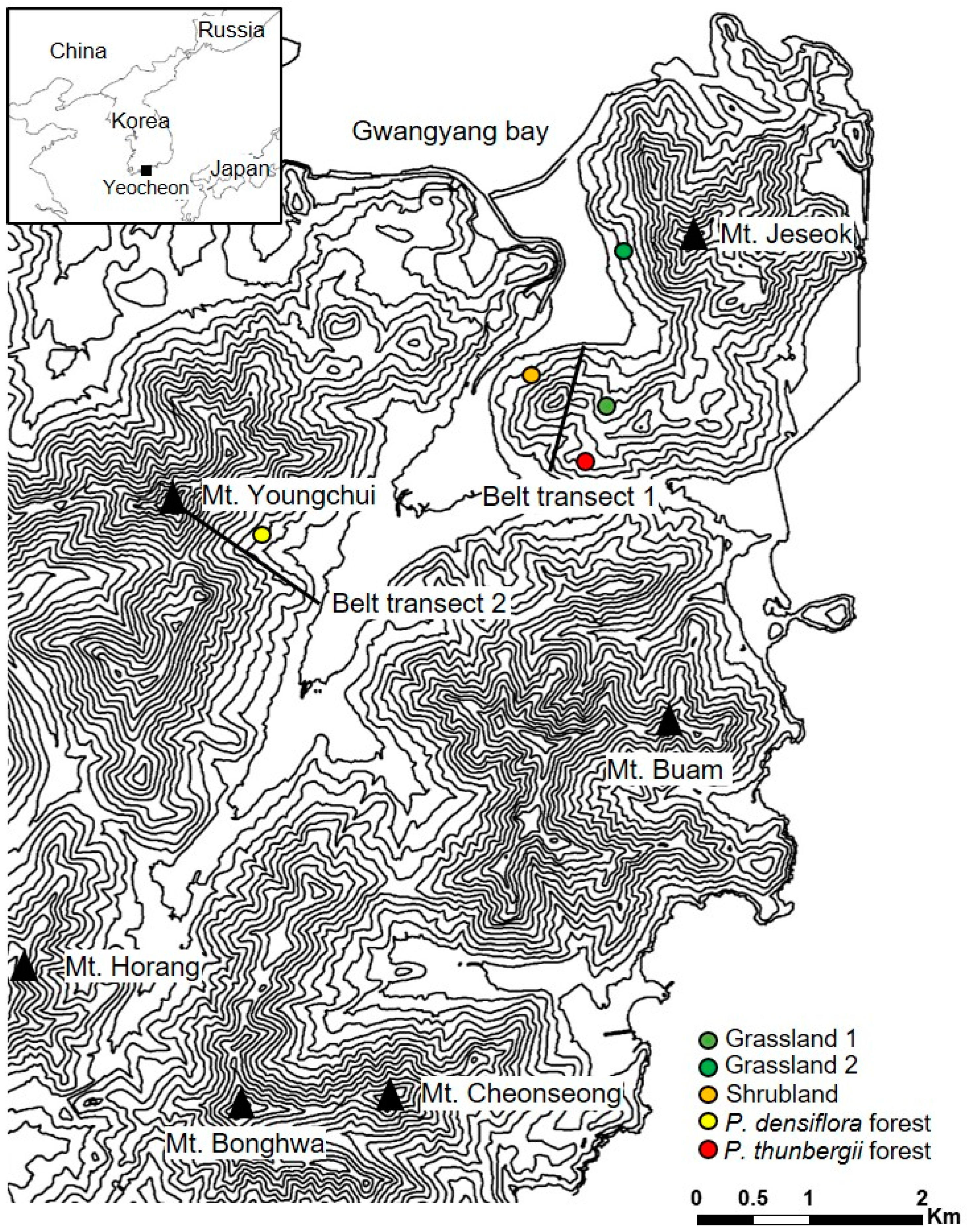
2.1. Study Area

This study was carried out around the Yeocheon industrial complex, located on the south coasts of the Korean Peninsula (Figure 1). This study area consisted of a watershed that forms three ridges. Two ridges, which are connected from Mt. Horang to Mt. Youngchui and from Mt. Cheonseong through Mt. Buamsan to Mt. Jeseok, run in the northeast direction, and a third ridge, which stretches from Mt. Cheonseong through Mt. Bonghwa to Mt. Horang, runs in the northwest direction, connecting the other two. In the valley located between the ridges that run in the northeast direction, there are agricultural fields and residences. The elevation of the study area ranges from 0 to 510 m (Mt. Youngchui) above sea level.
The parent rock of the mountainous areas consists mostly of igneous rock, and the flat land beside streams consists of alluvium. The soil in this area was classified into the alfisols, entisols, histosols, inceptisols, and ultisols, which developed on igneous bedrock [54].
The climate of this region is continental, with warm and moist summers and cold and dry winters. The mean annual temperature is 14.3 °C and the mean annual precipitation is 1428.0 mm (Korea Metrological Administration, 2020). Northeast and northwest winds dominate [55].
The forest vegetation of this area consisted of two major plant communities, the Pinus densiflora community in the inland area and the P. thunbergii community in the coastal area, before the construction of the industrial complex [56].
However, oak communities dominate areas where human interference is low and nature is thus well conserved. In this case, most areas are dominated by Quercus mongolica Fisch. Ex Ledeb. Community, but the Q. serrata Thunb. ex Murray community dominates the lower slope and the Q. variabilis Blum community tends to dominate the steep and infertile sites of the southern slope [57]. Celtis sinensis Pers. community remains as a remnant community near the coast [57].
Based on these results, we decided to use these oak communities and the C. sinensis community as the reference forest for comparing with the damaged vegetation types established close to the pollution source.
Yeocheon industrial complex is the representative heavy-chemical industrial complex of Korea constructed in the early 1970s. Thereafter, air pollutants that originated from many industrial facilities induced changes in the spatial distribution and structure of vegetation in the forest around the industrial complex.
Yeocheon industrial complex began construction in the early 1970s and is still expanding. Industrial activities focus on the heavy chemical industry, including the petrochemical industry. A major pollutant is SO2. The SO2 concentration in Yeocheon industrial complex increased continuously until 1991—the annual and daily means were 0.03 ppm and 0.06 ppm, respectively. Such severe air pollution not only caused vegetation degradation from forest to grassland and/or shrubland, but also led to soil acidification—the mean pH is 4.4 and the range is 3.5‒6.7 [16,17,58]. Moreover, the soil contains lower Ca2+ and Mg2+ contents (one-third to one-half) and two or three times higher Al3+ content than that in the healthy control area due to acidification [58].
However, these days, the ambient SO2 concentration stays at a level below 0.01 ppm, half the standard value (annual: 0.02 ppm, daily: 0.05), the target ambient concentration set by regulation [13], and the physicochemical properties of the soil are improved [59].
On the other hand, vegetation damage of this area was also interpreted as being due to hydrofluoride [60]. In this study, the fluoride concentration in needles of the P. thunbergii reflected well the spatial distribution of vegetation types. Grassland, shrubland, and forest tended to be established in the sites more than 400 ppb, 200 ppb, and below 100 ppb, respectively.

2.2. Experimental Design

This study was carried out to clarify the processes of forest decline and passive restoration, based on vegetation structure and dynamics that occurred over the last 50 years in the polluted forest around the Yeocheon industrial complex in southern Korea. The study area was designated to be within the boundary where the visible damage of vegetation was observed. The hypothetical belt transects were installed in the first and second ridges from the pollution source to clarify the spatial distribution of vegetation and the topographic conditions (Figure 1). The plots for vegetation survey were installed in two grasslands, shrubland, and two pine forests of P. thunbergii and P. densiflora, reflecting the vegetation damage (Figure 1). We did not secure the replicated plots for each vegetation type because of location constraints. Instead, we secured the various replicated subplots for each plot. The differences of species composition and diversity were compared among vegetation types that were different in damage degree and with the reference forests. To clarify the background of vegetation decline, we analyzed the annual ring growth of P. densiflora, which has an easily discernible annual ring. Furthermore, we analyzed the age structures of two dominant plants, P. densiflora and Styrax japonicas, to get information on the decline and regeneration of vegetation. Passive restoration was discussed based on the size class distribution of dominant woody plants in each vegetation type different in damage degree. The holistic changes of the area over the last 50 years were investigated by analyzing the landscape change.

2.3. Vegetation Survey and Data Processing

Vegetation surveys were carried out in 1991 and 2018. However, analyses of age distribution and annual ring growth, used to clarify when the forest decline started, were only performed in 1991. Field surveys were conducted from May to September in each year.
A landscape ecological map, including major vegetation types, was made based on aerial photograph interpretation (1:15,000 scale) and field checks. Field checks were done for the 1991, 2001, and 2018 maps. The final map was constructed with the ArcGIS program (ver. 10.0).
The stand profile was prepared by carefully depicting the horizontal and vertical distributions of the major plant species appearing in a hypothetical belt transect. This reflected the distance from the pollution source and changes in the topographic conditions. Spatial distribution of vegetation around the industrial area was discussed with special reference to the degree of air pollution estimated by distances from the pollution source and topographic conditions [16,17,18,33].
The vegetation survey was carried out by recording the cover class of plant species appearing in randomly installed quadrats of 2 × 2 m, 5 × 5 m, and 20 × 20 m in grassland, shrubland, and forest, respectively [61]. The vegetation survey was carried out in 45 subplots from June to August 1991. The numbers of subplots chosen for the vegetation survey were 9, 11, 8, 3, 6, and 8 for the Miscanthus sinensis var. purpurascens Anderss. (grassland), Phytolacca americana L. (grassland), S. japonicus (shrubland), Celtis sinensis Pers. (remnant forest), Pinus thunbergii Parl. (forest), and P. densiflora (forest) communities, respectively.
The 2018 survey was carried out on 48 subplots including 18, 9, 9, 5, and 7 subplots for the M. sinensis var. purpurascens (grassland 1), S. japonicus (shrubland), C. sinensis (forest), P. thunbergii (forest), and P. densiflora (forest) communities, respectively.
The reference forest, used for comparison, was designated as the oak (Quercus serrata Thunb. ex Murray, Q. mongolica Fisch. Ex Ledeb., and Q. variabilis Blum communities) forests, which are the representative late successional vegetation types in Korea [57]. The reference oak forests were selected in the area, which are far more than 10 km from the pollution source and therefore remain healthy. The reference forests are 50 to 100 years old, which means they are stable but not old growth. The numbers of subplots chosen for the survey for the reference oak forest were five, five, and two for the Q. serrata, Q. mongolica, and Q. variabilis communities, respectively.
All the plant species in each plot were identified using the Korea Plant Name Index [62]. Plant cover was recorded by applying the Braun‒Blanquet [63] scale. Each ordinal cover scale was converted to the median value of percent cover range in each cover class. Relative coverage was determined by dividing the cover fraction of each species by the total cover of all species in each plot and then multiplying the value by 100. Relative coverage was regarded as the importance value of each species. A matrix of importance values for all species in all plots was constructed and used as data for ordination using a detrended correspondence analysis (DCA [64]). Plant communities were named after dominant species and followed by subdominant species in the case of a mixed community.
To compare species diversity and dominance among sites, rank abundance curves [65,66,67] were plotted. The data used to obtain the species rank dominance curves were collected by selecting four plots randomly from each community.
For dominant tree and shrub species, stem diameters (at breast height for mature trees, DBH; or at stem base for seedlings and saplings below 1.3 m in height, D0) were measured and sorted by diameter classes. Stem diameters were measured for all tree and shrub species that appeared in four plots (20 × 20 m) selected randomly from each vegetation type. Stem diameter was measured with a tape ruler (mature tree) or Vernier calipers (seedlings and saplings) with mm precision.
Vegetation dynamics were analyzed by a frequency distribution of diameter classes of dominant tree and shrub species. The size distributions of trees are useful indicators for understanding the structures of tree populations and for predicting their dynamics [68,69,70]. The diameter class distribution of plant populations has generally been computed as frequency histograms [71]. Frequency distribution patterns of each diameter class indicate the potential change of the population in a plant community. A plant population where young individuals are numerous and mature ones are fewer is recognized as having a reverse J-shaped diameter distribution pattern [72,73]. It is recognized that a population that shows a reverse J-shaped distribution pattern can persist continuously [72,73,74,75]. On the other hand, a normal population pattern with fewer juveniles relative to adults is typically replaced by another population in the future [74,75], but a bimodal pattern is shown in a population that regenerates with periodic disturbance [76,77].
Age class distribution was investigated for P. densiflora and S. japonicus, which represent vegetation types before and after construction of the industrial complex in this area, respectively. Age was determined by counting the number of annual rings of core sample collected from stem of sample plants under a dissecting microscope. Core samples were collected 30 cm above the ground surface. The time it took to reach 30 cm was determined as five and three years for P. densiflora and S. japonicus, respectively [51,78]. Age distribution was investigated for all individuals of P. densiflora and S. japonicus that appeared in four plots (20 × 20 m) selected randomly from the two vegetation types.
Core samples for estimating the tree age and analyzing the growth of annual rings were collected by an increment borer. The growth of annual rings was measured with calipers under a dissecting microscope with a 0.05 mm precision. Core samples for the analysis of radial growth were collected from 10 individuals selected randomly from the P. densiflora individuals that survived severe air pollution damage in the early stage when the industrial facilities began to be operated.
Landscape structure and change were interpreted by analyzing landscape ecological maps constructed before and in the 4th, 17th, 27th, and 44th years after the construction of the industrial complex.

2.4. Statistical Analyses

All statistical analysis was carried out using SPSS (Statistical Package for the Social Sciences) 24 software package. The t-test was applied for comparing the differences of the annual ring growth of P. densiflora between the suppressed and non-suppressed periods. Leneved’s test was performed to determine the homogeneity of variance in the two groups [79].
Detrended correspondence analysis (DCA) was used to identify differences in species composition among vegetation types. DCA is a multivariate technique that maximally separates species distribution in ordination space; stand and species placements are constrained to be linear combinations of environmental variables [80]. This analysis was conducted to compare species composition among vegetation types and between the survey years 1991 and 2018.

3. Results

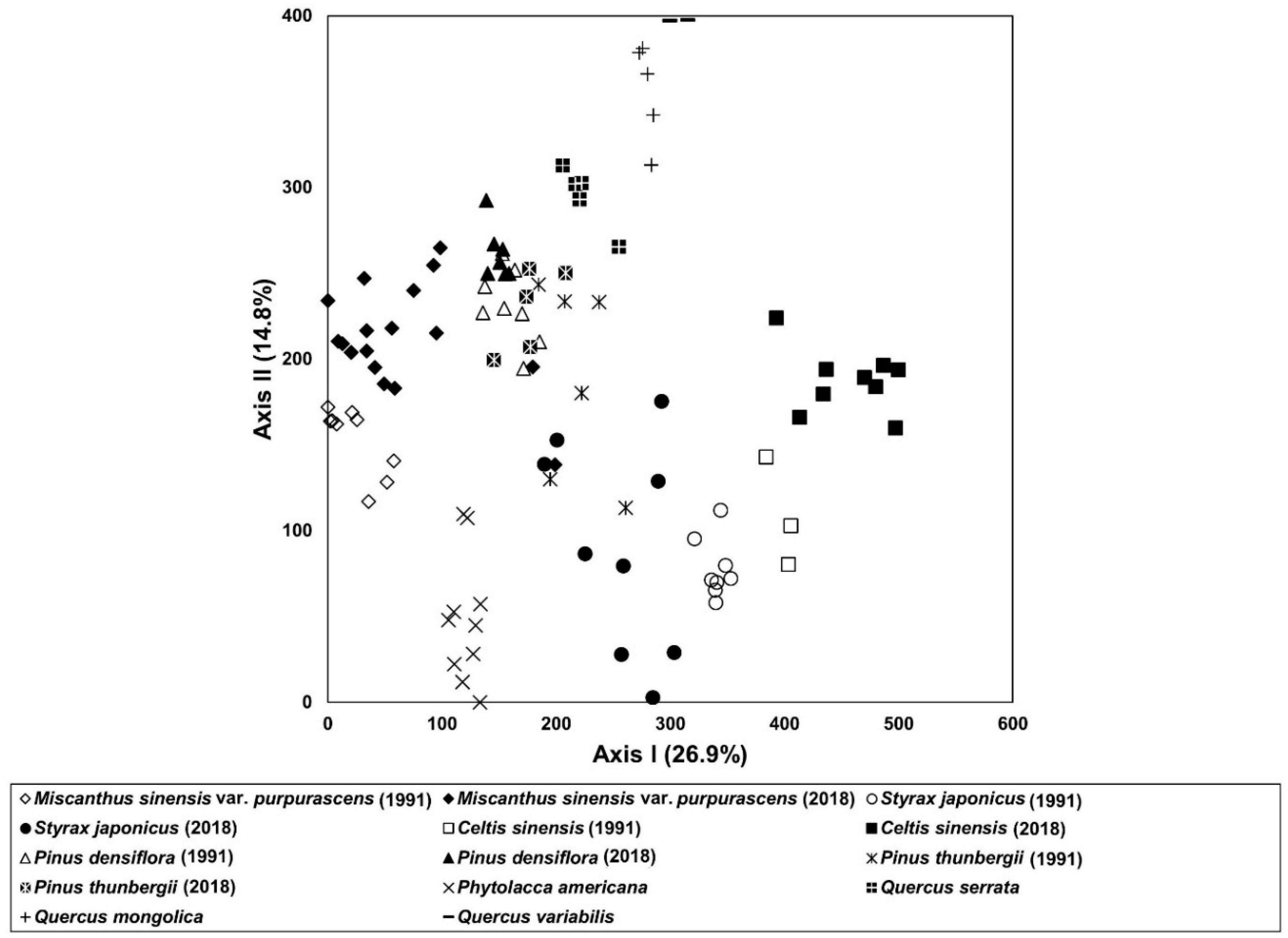
3.1. Vegetation Sequence

The result of a DCA ordination of stands based on vegetation data tended to be divided into the upper and the lower parts on the diagonal line that axis I and axis II form (Figure 2). Plant communities arranged in the upper part tended to be established in the upper part of the hill slope, which is far from the pollution source located near the coast, while those in the lower part were distributed in the lower part of the slope, which is closer to the pollution source and coast. In the upper part, M. sinensis var. purpurascens (grassland), P. thunbergii (forest), P. densiflora (forest), and the reference oak stands were arranged in the mentioned order in the diagonal direction. In the lower part, P. americana (grassland), S. japonicus (shrubland), and Celtis sinensis Pers. (forest) stands were arranged in the mentioned order in the same direction as that in the upper part.
In the result based on data collected in 2018, stands of M. sinensis var. purpurascens tended to be closer to the forest stands composed of P. thunbergii and P. densiflora, whereas stands of P. thunbergii and P. densiflora little changed. Stands of S. japonicus became far from the forest stands, which were composed of C. sinensis and scattered. Stands of C. sinensis became farther from stands of S. japonicus; stands succeeded from P. americana stands were arranged close to stands surveyed in 1991 and S. japonicus stands. On the other hand, stands of P. americana were succeeded by C. sinensis.

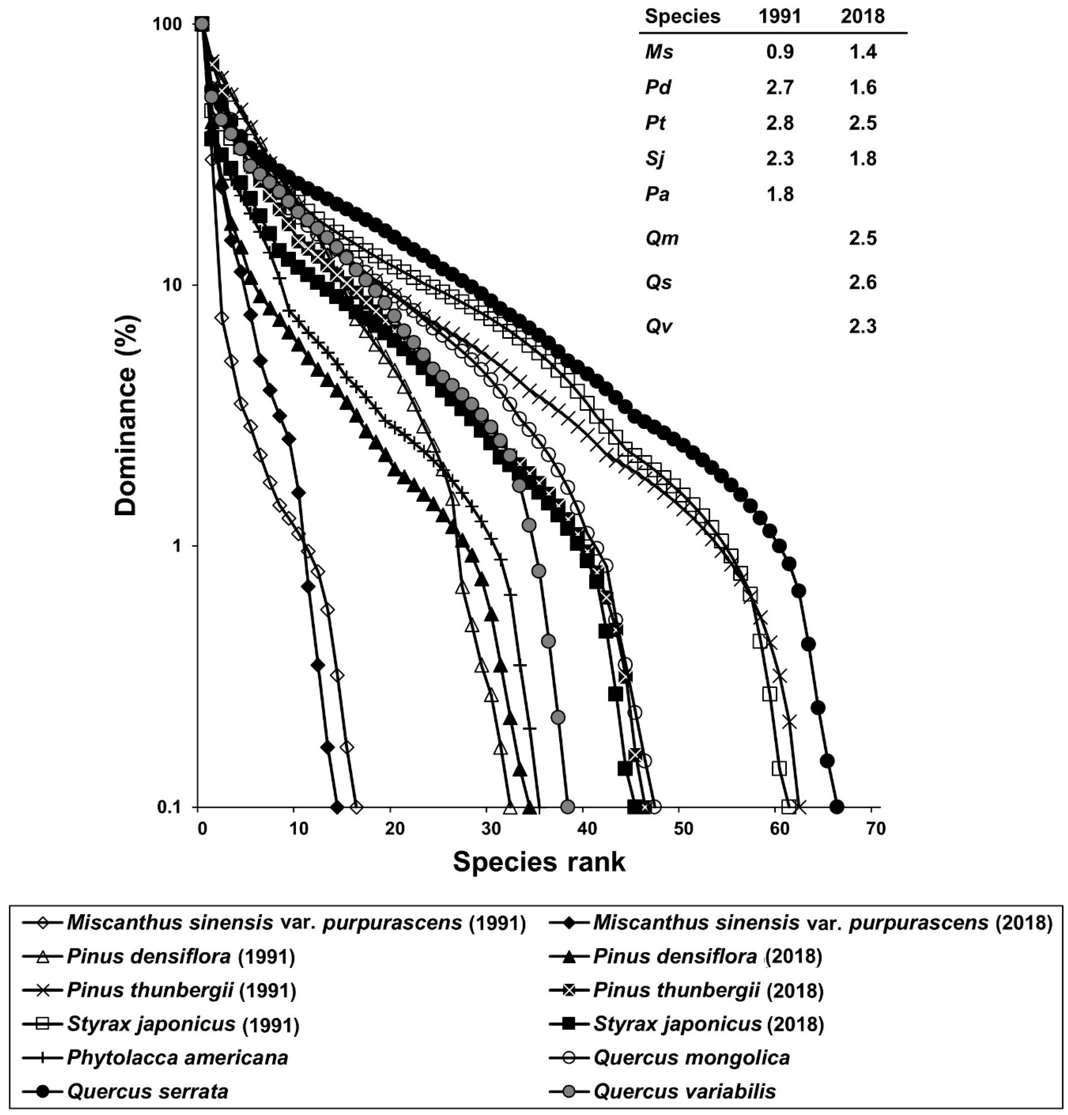
3.2. Species Diversity

In the data from 1991, species richness was the lowest in the M. sinensis var. purpurascens community and the highest in the S. japonicus and P. thunbergii communities; the P. americana and P. densiflora communities were at a medium level. Compared with the reference oak communities, the species richness of M. sinensis var. purpurascens and P. densiflora communities was the lower but those of S. japonicus and P. thunbergii communities were similar to each other (see the x-axis in Figure 3).
In the data from 2018, the order of species richness did not change. Comparing the species richness between survey years, those of the S. japonicus and P. thunbergii communities decreased greatly but those of the M. sinensis var. purpurascens and P. densiflora communities changed little.
The results compared by the slope of the species rank dominance curve, which indicates the evenness, showed a similar trend (Figure 3).
The results compared based on Shannon index showed a similar trend (Figure 3).

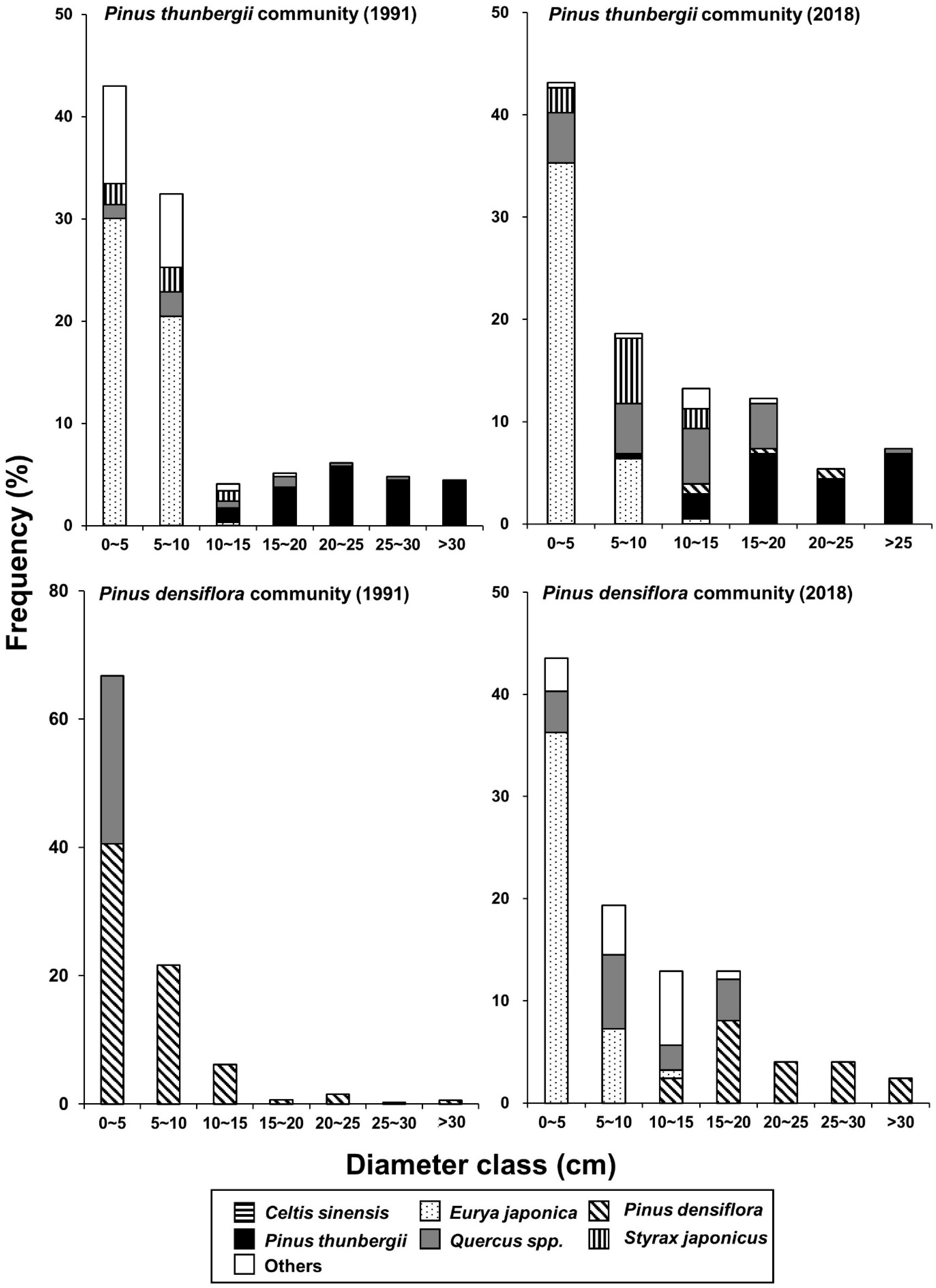
3.3. Vegetation Dynamics

In the 1991 survey for grassland 1, oaks, which are usually Quercus serrata, appeared in a state of undergrowth below dominant M. sinensis var. purpurascens, and the density was also very low. The size class distribution of them showed a reverse J-shaped pattern. In the 2018 survey, Quercus spp. grew to shrub size but not many new seedlings were recruited; therefore, the size class distribution showed a J-shaped pattern (Figure 4).
In grassland 2, which is located near the northern coast, C. sinensis appeared. C. sinensis grew bigger than oaks and their size class distribution showed a reverse J-shaped pattern in which new seedlings were recruited continuously in the 2018 survey (Figure 4).
In the size class distribution diagram for the dominant species composing S. japonicus stands, S. japonicus showed a reverse J-shaped distribution pattern. Quercus spp. had a frequency of over 10% in diameter classes below 10 cm, but its frequency in other classes was low. In this diagram, Pinus spp. also appeared, but their frequency was also low. In the 2018 survey, the S. japonicus population still showed a reverse J-shaped pattern, except in the diameter class below 5 cm. Quercus spp. appeared in all diameter classes evenly; mature trees more than 30 cm also appeared, although the frequency was not so high (Figure 4).
In the size class distribution diagram for dominant species composing a P. thunbergii forest located on the opposite slope of the pollution source, the P. thunbergii population showed the normal distribution pattern, with fewer juveniles relative to adults, whereas the Eurya japonica Thunb. population showed a reverse J-shaped distribution pattern in diameter classes below 15 cm. Quercus spp. usually appeared in the lower diameter classes, but the density was very low. S. japonicus was restricted to diameter classes below 15 cm and showed a frequency distribution similar to that of Quercus spp. In the 2018 survey, the size class distribution diagram changed little, but the oak density increased a bit (Figure 4).
In the size class distribution diagram for dominant species composing P. densiflora forest, the P. densiflora population showed a reverse J-shaped pattern whereby seedlings and saplings are recruited continuously. Quercus spp. appeared only in the diameter classes below 5 cm. In the 2018 survey, the P. densiflora population changed to a normal distribution pattern, with fewer juveniles than adults. The E. japonica population as an evergreen shrub appeared at a very high density below 10 cm and showed a reverse J-shaped pattern. Quercus spp. showed a reverse J-shaped pattern, although the density was relatively low (Figure 4).

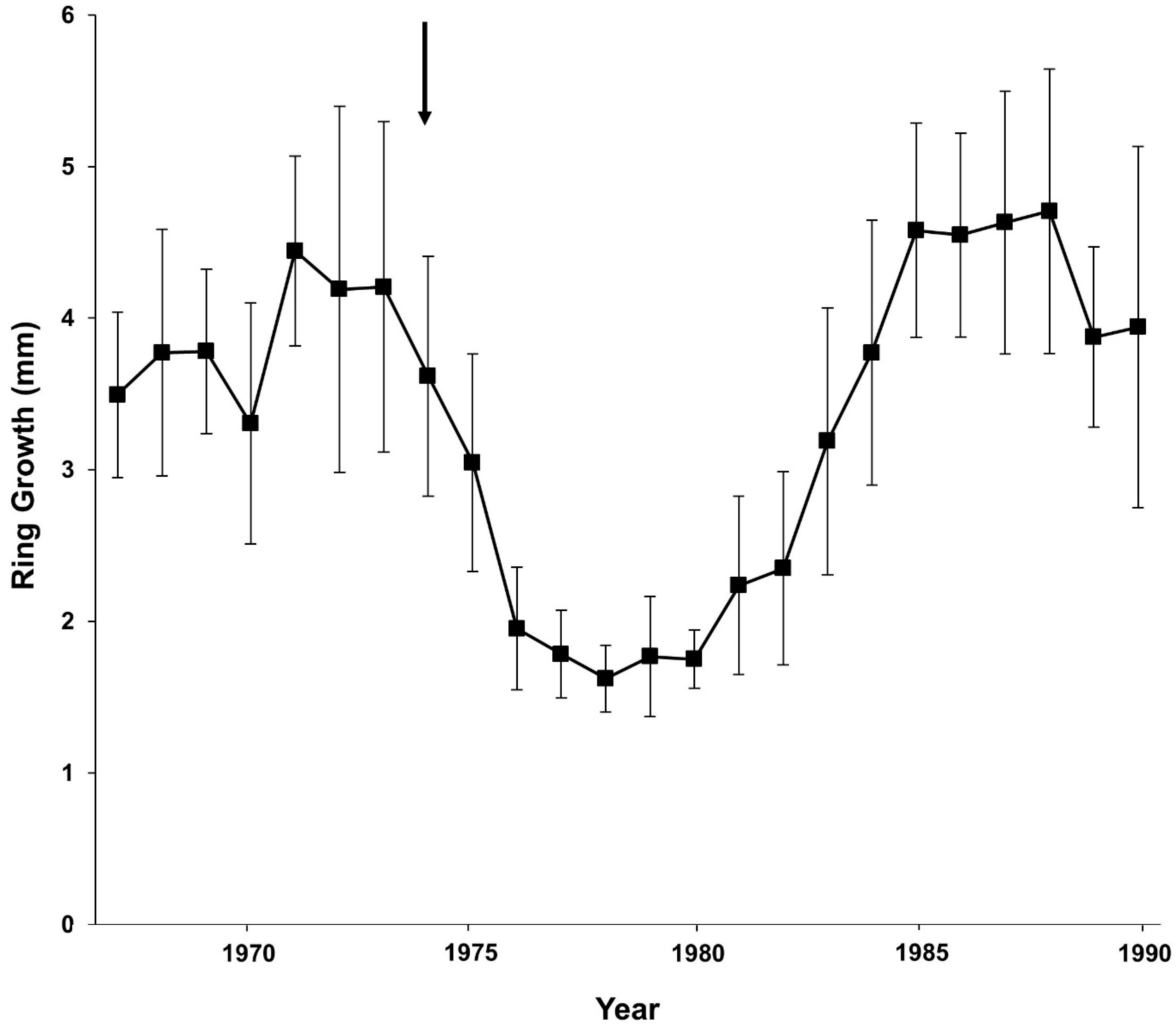
3.4. Yearly Changes in Annual Rings

The annual ring growth of pine trees that survived air pollution damage was suppressed for about 10 years after industrial facilities began to operate in this area, but since then they tended to recover (Figure 5). It was supposed that the suppressed growth originated from air pollution and the improvement of growth since then was due to the release from competition after the selective death of neighboring trees and the mitigation of air pollution [51,73].
Annual ring growth during the suppressed period showed a significant difference from that of the non-suppressed period (Table 1).

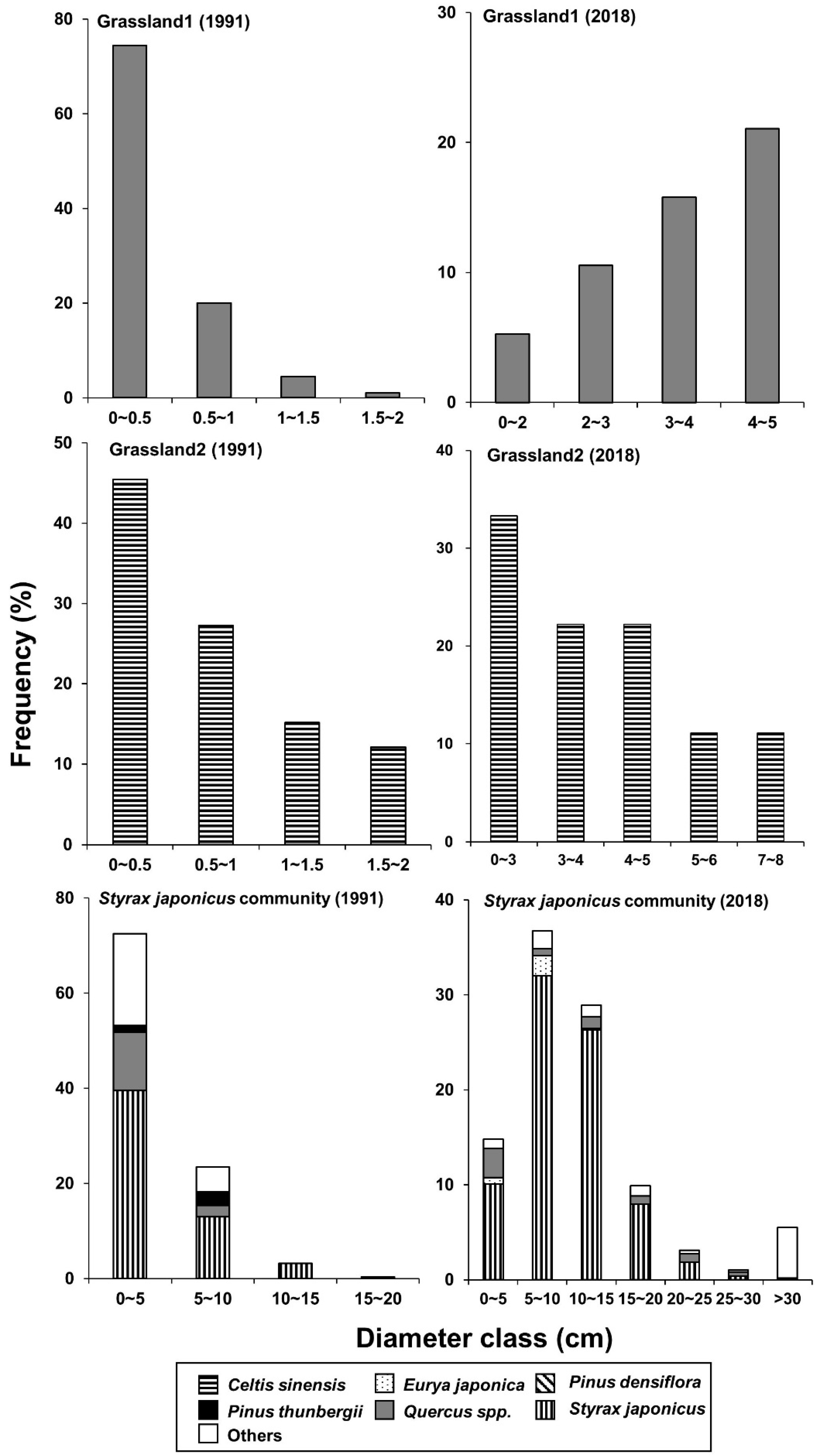
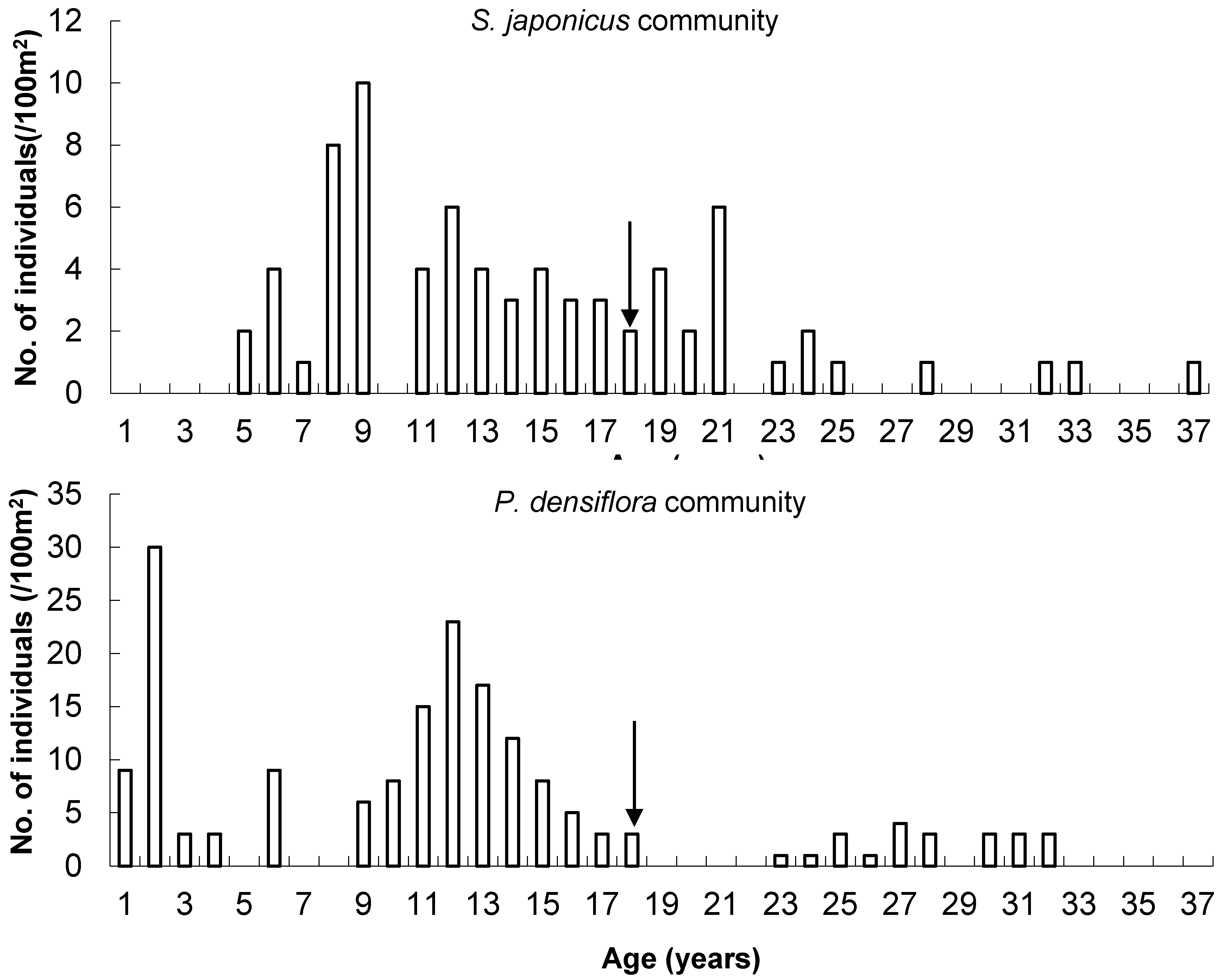
3.5. Age Distribution of Two Dominant Species

The age of S. japonicus ranged from five to 37 years (Figure 6). Individuals younger than 18 years, established after the construction of the industrial complex, made up more than 70% of the total.
In an age class distribution diagram of the P. densiflora community (Figure 6), the ages of the pine trees ranged from one to 33 years. Those aged 10 to 15 years old accounted for more than 40%.
The period when young individuals were recruited in both the S. japonicus and p. densiflora communities corresponded to the period when the annual ring growth of the pine trees that survived air pollution was suppressed (Figure 6). These results suggest that most individuals in these two communities are the products of air pollution damage and natural regeneration of damaged forest.

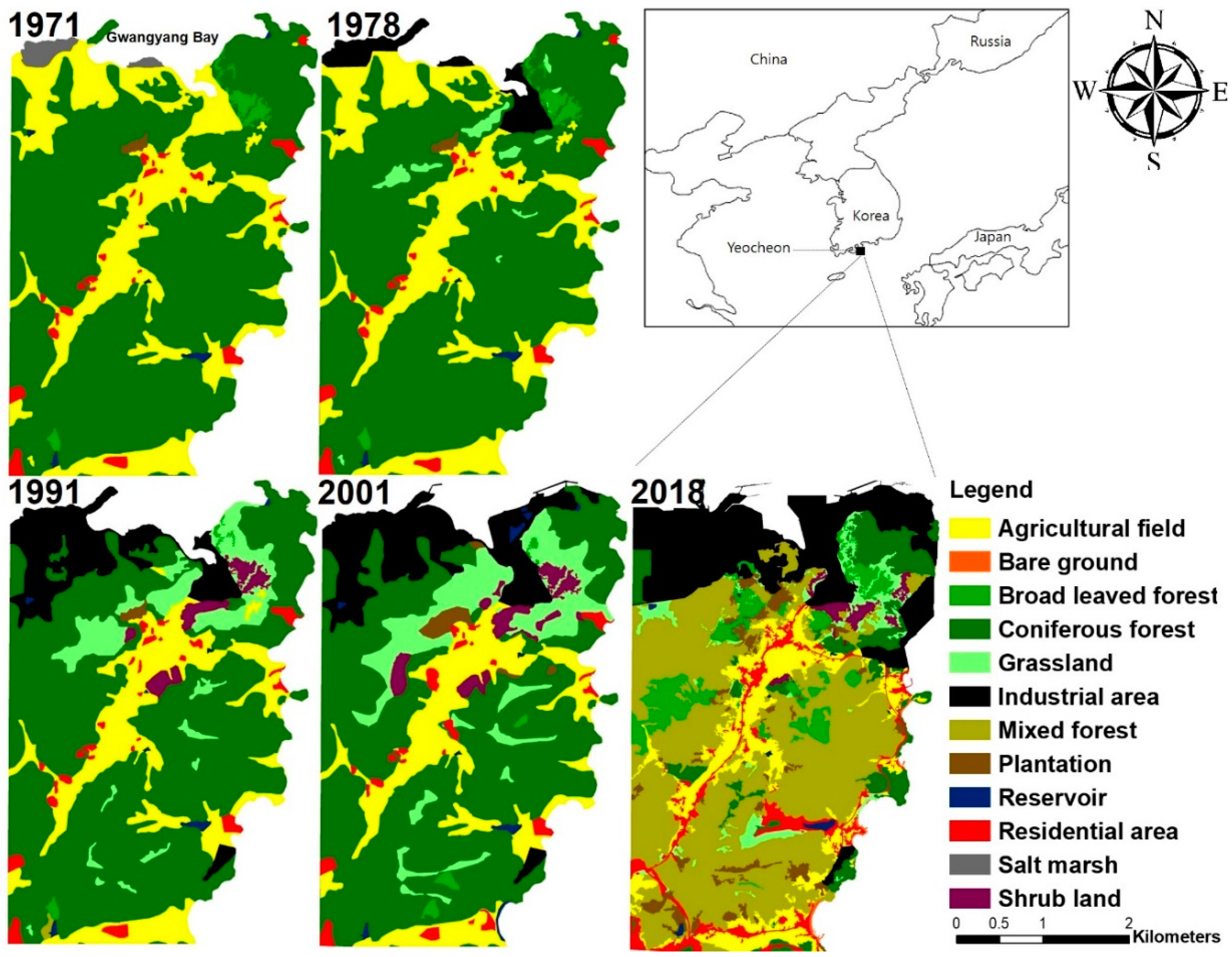
3.6. Landscape Structure and Change

The land use pattern in this area is divided clearly depending on the topographic conditions. Upland was covered with forest, whereas lowland was dominated by agricultural field until the early 1970s. However, since then, an industrial area appeared as a new landscape element. The industrial area was restricted to the northern lowland in the early 1970s, but has expanded continuously since then.
Forest in this area before the construction of industrial complex was usually coniferous, dominated by the Korean red pine (P. densiflora) community and partially mixed with black pine (P. thunbergii) depending on the site [56]. Grassland began to appear near the northern part of the industrial complex in the late 1970s. The area occupied by grassland increased continuously throughout the 1990s and early 2000s but decreased in recent years. Grassland appeared on the ridge distant from the industrial area as well. Shrubland appeared in 1991; its area increased up to the early 2000s but decreased in recent years, as was the case with grassland. In 2018, the change from coniferous forest to mixed or deciduous forest was remarkable. In addition, the plantation and residential area also increased (Figure 7).
In 1971, before the construction of the industrial complex, coniferous forest dominated by P. densiflora occupied the largest area at 72.3%, and agricultural fields (23.6%), residential areas (2.2%), broad-leaved forests (1.4%), and so on followed.
By 1978, the landscape structure was little changed, except that industrial areas (3.5%) and grassland (1.6%) were new categories.
In 1991, the 17th year after the industrial facility was constructed, the areas occupied by coniferous forest and agricultural fields were reduced to 55.4% and 14.9%, respectively, whereas those of grassland and industrial increased greatly to 14.7% and 9.4%, respectively. On the other hand, shrubland dominated by the S. japoncus community (1.8%) appeared for the first time in 1991.
In 2001, coniferous forest decreased to 53.1%, whereas the industrial area increased to 11.9%. The area of shrubland (2.6%) also increased, although not so noticeably.
In 2018, the areas of coniferous forest and grassland decreased greatly to 8.1% and 3.8%, respectively; mixed forest (42.2%) increased greatly, and broad-leaved forest (6.3%) and plantation (3.3%) also increased. The area of agricultural field decreased more, whereas that of industrial area increased more. The area of shrubland (1.3%) decreased a little. In this period, the increase in mixed forest was due to the increase in broad-leaved forest composed of oaks and C. sinensis. The former was usually established above the mid-slope, while the latter was in lowland close to the northern coast.
The landscape elements identified in each investigated year and landscape change are summarized in Appendix A.

4. Discussion

4.1. Characteristics and Establishment Background of Vegetation Around the Yeocheon Industrial Complex

In a heavily industrialized area, the effects of high levels of atmospheric pollution may be demonstrated quite visibly in surrounding forests and other ecosystems [1,2,81,82,83,84]. In such cases of intense air pollution, vegetation may suffer extensive mortality, resulting in dramatic changes in species composition, reductions in biomass and productivity, erosion of soil, nutrient loss, and changes in microclimatic and hydrological regimes. In severe cases, the perturbation can result in extreme ecosystem simplification and almost complete denudation [1,2,4,26,85].
Grassland, dominated by M. sinensis var. purpurascens, P. americana, etc., and shrubland, dominated by S. japonicus, which emerged since the construction of the industrial complex in this study area, reflect such phenomena (Figure 7). A structural change from forest to shrubland or grassland means a reduction in biomass (Figure 7) and vegetation simplification (Figure 4).
M. sinensis var. purpurascens is extremely shade-intolerant, so it cannot form a pure stand throughout this wide area if there is no bare ground. P. americana is an exotic plant. It is rare and also cannot form a pure stand of wide area if there is no severe disturbance. However, the density increased closer to the pollution source and it formed pure stands in sites near the pollution source. S. japonicus has similar ecological attributes to those plant species. NIER [86] classified S. japonicus as a species sensitive to pollution, whereas NIER [87] did it as a tolerant species. This difference might be related to the period in which the observation is conducted. As shown in our results (Figure 6 and Figure 7, Table 1), this species appeared since the construction of the industrial complex. This means that this species is tolerant of the environmental conditions in this area. In an experimental study of exposure to SO2, S. japonicus was sensitive to SO2 exposure, showing rapid necrosis and leaf shedding [58]. However, the damaged plants produced new leaves a few days later. This implies that this plant is a resilient to air pollution rather than a tolerant species [88]. C. sinensis, which emerged in grassland 2, also showed the characteristics of a resilient species.
Direct damage to vegetation near point sources is characterized by a spatial pattern of exponentially decreasing intensity with increasing radial distance. Acute effects on vegetation may occur in areas immediately surrounding sources of emitted pollutants, while lower-level, regional effects may be much more widespread, but difficult to document. The direct and indirect effects of air pollutants on forest ecosystems depend on numerous complex variables, including the intensity of exposure; mitigating environmental conditions; and the inherent susceptibility of affected populations, species, and communities [7,89,90]. The spatial distribution of vegetation in this area, which was dominated by the distance from the pollution source and topography, reflects these trends (Figure 7 and Figure 8).
The spatial distribution of vegetation along the distance from the pollution source tended to be in the order of grassland, shrubland (dominated by S. japonicus community), and forest (dominated by P. thunbergii and P. densiflora communities) (Figure 8). Such a distributional trend might be related to the air pollutants being transported with the land and sea breeze as it is a coastal area bordering Gwangyang bay (Figure 1 and Figure 7) [17]. Grassland was dominated by the Miscanthus sinensis var. purpurascens and Phytolacca americana communities. This M. sinensis var. purpurascens community is a vegetation type that emerged from damage due to severe air pollution. Shrubland was dominated by the S. japonicus community. This community is established in areas near to the pollution source, but the effects of air pollution are mitigated by topographic conditions. Forests, dominated by P. thunbergii and P. densiflora communities, were established in the areas which are distant from the pollution source or experience more mild air pollution due to the topographic conditions, such as at the foot of the slope opposite the pollution source (Figure 8).
This phenomenon was also reflected on the result of ordination based on the vegetation data (Figure 2). In the result of stand ordination, vegetation types established in the inland area were arranged above the diagonal line that axis I and axis II form, whereas vegetation types established in the coastal area were below the line. The vegetation types changed from grassland through two pine forests to the late successional oak forests above the line, and from grassland through shrubland and some pine forests to the C. sinensis forest in the lower part as move along the diagonal direction on the plane that axis I and axis II form. From these results, we could interpret that axis I means the successional stage and axis II reflects the distance from the coastal area (Figure 2). That is, the distribution and composition of vegetation in this area are usually dominated by the distance from the source of pollution, and the influence of the sea is partial. In particular, the fact that the result of ordination reflects the successional stage means that pollution affects not only the distribution of vegetation but also the progression of the succession. Previous studies carried out in this area revealed that soil acidification, changes of physicochemical properties of soil due to that, and visible damage of plants are usually dominated by the distances from the pollution source [17,18,32,37]. Considering the facts synthetically, axis I indicates the degree of pollution and vegetation degradation due to the distance from the pollution source.
The spatial distribution of vegetation and the difference of species composition among vegetation types do not have a statistical significance because we did not secure the replicated belt transects and plots for each vegetation type due to location constrains. However, we can read those trends from the spatial distribution diagram (Figure 8), the result of ordination (Figure 2), and the vegetation map (Figure 7).

4.2. Relationship Between Environmental Factors and Spatial Distribution of Vegetation

In most studies on point sources of air pollution, there is a generic observation that ecological damage becomes progressively less severe as the distance from the source increases. This pattern closely tracks the gradients of pollution, which are characterized by a roughly exponential decrease in intensity as the distance from the source increases [1].
If a forested ecosystem is affected by air pollution, the canopy level is generally impacted first and is stripped away. As the canopy declines, shrubs and then the ground vegetation are affected. This syndrome of the sequential death of horizontal strata of the terrestrial vegetation, described as a “peeling off” or “layered vegetation effect” by Gordon and Gorham [91], was clearly observed in this area (Figure 8).
Under long-term pollution stress, the ecosystem of this area was characterized by biological simplification. In addition, pollution-tolerant species are not usually present or are rare, since unpolluted habitat dominates the vegetation of this area. Most of them began to emerge as industrial facilities were opened in this area (Figure 6 and Figure 7). Forest remnants remained in sites where the topography gave some protection from fumigation. They were on relatively protected, mesic, lower slopes of hills (Figure 8).
Grassland and shrubland emerged as a result of severe air pollution damage (Figure 5, Figure 6 and Figure 7), and forest remnants that survived the damage were impoverished around the industrial complex (Figure 3 and Figure 8). A sharp decrease in species richness was observed in grassland, and richness also decreased in P. densiflora forest (Figure 3). The decrease in grassland was due to the simplification of the vegetation structure from “layered vegetation effect” [91]. The high density of E. japonica indicated that it was tolerant to air pollution [16,17,33,58]. On the other hand, the species richness of the S. japonicus and P. thunbergii communities was high—at a similar level as the reference oak communities (Figure 3). This result can be explained based on the intermediate disturbance hypothesis that species diversity is maximized when ecological disturbance is neither too rare nor too frequent [92].

4.3. Future Prospects Based on Vegetation Dynamics

In grassland 1, diameter class distribution of Quercus spp. in grassland showed a reverse J-shaped pattern, although the density was very low (ca. 200 individuals·ha−1). In the 2018 survey, the density increased to 350 individuals·ha−1 and the diameter also increased to the level of the shrub layer, but new seedlings were not recruited often, and therefore the size class distribution showed a J-shaped pattern (Figure 4).
In grassland 2, which is located near the northern coast, C. sinensis appeared as a successor tree in the 1991 survey. C. sinensis grew a little bigger than oaks and the size class distribution showed a reverse J-shaped pattern in the 2018 survey (Figure 4).
S. japonicus, a dominant species of the S. japonicus community, showed a reverse J-shaped pattern in the 1991 survey. Quercus spp. also showed a reverse J-shaped pattern in this stand, but their density was very low compared with S. japonicus. In the 2018 survey, recruitment of S. japonicus seedlings decreased but still showed a reverse J-shaped pattern. Quercus spp. appeared evenly in all diameter classes and mature trees over 30 cm also appeared, although the frequency was still low. Pinus spp. appeared in 1991 but disappeared in 2018.
In the P. thunbergii forest, the frequency distribution of the diameter class of the P. thunbergii population showed a normal pattern without seedling recruitment in both the 1991 and 2018 surveys. The density of Quercus spp. as successor trees was very low in the 1991 survey but increased in 2018. However, shrubby plants, such as Eurya japonica and S. japonicus, which are tolerant or resilient to air pollution, dominated the smaller diameter classes.
In the P. densiflora forest, the P. densiflora population showed a reverse J-shaped pattern in 1991 but changed to a normal distribution in 2018. On the other hand, Quercus spp., which appeared only in the diameter class below 5 cm in 1991, showed a reverse J-shaped pattern, although their density was relatively low in 2018. Even in this forest, two shrubby plants dominated the smaller diameter classes.
From those results, we could deduce that oaks or C. sinensis would be the potential dominant species in this region (Figure 4). In grassland, both the density and size of oaks increased in 2018 compared with 1991, although the density was still very low. Meanwhile, the C. sinensis emerged as a successor tree in grassland located near the coast. Even in the results of S. japonicus stands collected in 2018, the density of oaks increased, and some individuals grew to the canopy level. In forests dominated by the P. thunbergii and P. densiflora communities, oaks showed potential to be successor trees, but their density was relatively low. Moreover, shrubby plants dominated smaller diameter classes with very high density. Therefore, whether the vegetation of this area, which is still affected by air pollution from the industrial complex, could be succeeded by oak forest in the late successional stage along the normal successional trajectory or not depends on the intensity of pollution; the environmental quality in this area is getting better [13,78]. Before industrialization, this area was covered in mixed pine forests [56]. Such pine domination was due to frequent human disturbances typical of rural areas in Korea—for example, cutting, pruning, weeding, needle scraping to get timber, fuel, organic fertilizer, feed for livestock, etc. [93,94]. However, socioeconomic changes due to the rapid economic growth since the 1980s vanished these land uses in Korea. Consequently, many coniferous forests are in succession to broad-leaved forest, including oak forest, these days; a similar successional trend was confirmed in this industrial area as well.

4.4. Implications for Restoration

Air pollutants emitted in the processes of industrial activities simplify the vegetation structure through layered vegetation effects, which parallel the pollution intensity [91,95] and further weaken the function [1,2,4,16,17,18,33,50]. Vegetation fulfills diverse ecological functions, including air purification [7,96,97]. Therefore, the structural simplification and functional weakening of vegetation aggravates pollution damage [1,7,16,17,18,33,50]. From this viewpoint, the recovery of ecosystem services through vegetation restoration is a necessity.
Restoration is the process of assisting in the recovery and management of ecological integrity [98,99]. A restoration project can range from a very simple task to a very complex science. The methods are divided as follows depending on the degree of human intervention [100]. The first method relies on the natural recovery ability of the ecosystem. The second one facilitates vegetation recovery, at least by investing bioenergy. The last one is restoring the ecosystem by investing bioenergy positively, such as through the planting of seedlings.
In order to restore a degraded ecosystem in a polluted environment, interception of pollutants, the amelioration of the polluted environment, the selection of pollution-tolerant plants, the determination of the best planting methods, etc., are required [16,17,18,33,50,101]. The structure of the plant community is determined in response to the abiotic environment that is established. Therefore, clarifying the structural characteristics of the plant communities that are established in the polluted environment could provide crucial information that can be used to determine the methods and kinds of plants to be introduced to restore the vegetation [98].
As mentioned above, woody plants, which have the potential to be dominant in this region, appear on the vegetation floor in grassland. Even in shrubland or pine-dominated forest where there are better environmental conditions than in grassland, they keep their status as potentially dominant. This implies that natural vegetation can be recovered through passive restoration [102,103]. However, vegetation change is far slower than during active restoration [18] or after the succession of pine forest, which involved pine gall midge damage [51]. Such a situation suggests that restoration, the second of the three methods that Bradshaw [100] introduced, would be suitable for this area. When restoration was practiced by introducing potential dominants, which were selected as tolerant species through several experimental procedures [16,17], it showed restoration effects in terms of a change in species composition and an increase in biodiversity [18].

5. Conclusions

We reached to the following conclusion from the analyses on the spatial distribution of vegetation, differences in species composition and diversity among vegetation types different in damage degree, vegetation dynamics, the age structure and annual ring growth of two dominant plant species, and the landscape change that occurred in this area over the last 50 years.
The distribution and composition of vegetation are affected by the distance from a source of pollution. Our results also reflected the successional stage of the plant communities, which means that pollution affects not only the distribution of vegetation, but also the progression of the succession.
The results of analyses on the annual ring growth and the age structure of two dominant species showed that the establishment of shrubland and forest—composed of shade-intolerant plants, such as pines—is a result of vegetation decline due to pollutants discharged after the construction of the industrial complex, and regeneration of the gap occurred from the vegetation’s decline.
The size class distribution of dominant woody plants indicated that it was likely that all vegetation types, including grassland, shrubland, and pine forest, would be succeeded by deciduous broadleaved forests in the late successional stage as the effects of pollution diminish. These results can be interpreted as the result of the passive restoration that occurred as the environmental conditions improved due to socioeconomic changes. Furthermore, this trend is also confirmed by the analysis of landscape changes.

Author Contributions

Writing—original draft, H.L.; Investigation, Data curation and Formal analysis, B.S.L., D.U.K., A.R.K., J.W.S., J.S.M., J.H.K.; methodology and software, C.H.L.; Conceptualization, Supervision, Writing—review & editing, C.S.L.; All authors have read and agreed to the published version of the manuscript.

Funding

This research received no external funding.

Conflicts of Interest

There are no potential conflicts of interest to declare.

Appendix A. Landscape Change Progressed for the Last 50 Years around the Yeocheon Industrial Complex

Landscape Element19711978199120012018
km2%km2%km2%km2%km2%
Forest
Broad leaved forest0.61.10.61.10.20.30.30.63.66.3
Coniferous forest38.571.437.869.933.261.030.453.74.68.1
Mixed forest----0.50.9--24.042.2
Plantation0.10.3--0.10.30.61.01.93.3
Shrub land----1.12.01.52.70.71.3
Grassland--0.81.54.37.96.411.32.23.8
Subtotal39.272.739.272.539.372.339.269.336.965.0
Others
Agricultural field12.723.611.621.48.515.58.515.06.110.8
Bare ground- - - - 0.10.2
Industrial area- 1.93.65.39.86.812.110.418.4
Reservoir0.20.40.20.40.20.40.40.80.20.3
Residential area1.22.21.22.21.12.11.62.93.05.3
Salt marsh0.61.2- - - -
Subtotal14.727.314.927.515.127.717.330.719.935.0
Total54.0100.054.1100.054.5100.056.5100.056.8100.0

References

  1. Freedman, B. Environmental Ecology: The Ecological Effects of Pollution, Disturbance, and Other Stresses; Elsevier: Amsterdam, The Netherlands, 1995. [Google Scholar]
  2. Gunn, J.M. Restoration and Recovery of an Industrial Region: Progress in Restoring the Smelter-Damaged Landscape near Sudbury, Canada; Springer Science & Business Media: New York, NY, USA, 1995. [Google Scholar]
  3. Seinfeld, J.H.; Pandis, S.N. Atmospheric Chemistry and Physics: From Air Pollution to Climate Change, 3rd ed.; John Wiley & Sons: Hoboken, NJ, USA, 2016. [Google Scholar]
  4. Smith, W.H. Air Pollution and Forests: Interactions between Air Contaminants and Forest Ecosystems; Springer Science & Business Media: Berlin, Germany, 1990. [Google Scholar]
  5. Morecroft, M.D.; Cape, J.N.; Parr, T.W.; Brown, J.C.; Caporn, S.J.M.; Carroll, J.A.; Emmett, B.A.; Harmens, H.; Hill, M.O.; Lane, A.M.J.; et al. Monitoring the impacts of air pollution (acidification, eutrophication and ground-level ozone) on terrestrial habitats in the UK: A Scoping Study; Environment and Heritage Service: Belfast, Northern Ireland, 2005; 293p. [Google Scholar]
  6. Rockström, J.; Steffen, W.; Noone, K.; Persson, Å.; Chapin, F.S., III; Lambin, E.; Lenton, T.M.; Scheffer, M.; Folke, C.; Schellnhuber, H.J. Planetary boundaries: Exploring the safe operating space for humanity. Ecol. Soc. 2009, 14, 32. [Google Scholar] [CrossRef]
  7. Gheorghe, I.F.; Ion, B. The effects of air pollutants on vegetation and the role of vegetation in reducing atmospheric pollution. In The Impact of Air Pollution on Health, Economy, Environment and Agricultural Sources; Khallaf, M., Ed.; InTech: London, UK, 2011; pp. 241–280. ISBN 978-953-307-528-0. [Google Scholar]
  8. Kelly, F.J.; Fussell, J.C. Air pollution and public health: Emerging hazards and improved understanding of risk. Environ. Geochem. Health 2015, 37, 631–649. [Google Scholar] [CrossRef] [Green Version]
  9. Spiegel, J.; Maystre, L.Y. Environmental pollution control and prevention. In Encyclopaedia of Occupational Health and Safety; International Labour Office: Geneva, Switzerland, 1998; Volume 4, Chapter 55- Environmental Pollution Control. [Google Scholar]
  10. Pirrone, N.; Cinnirella, S.; Feng, X.; Finkelman, R.B.; Friedli, H.R.; Leaner, J.; Mason, R.; Mukherjee, A.B.; Stracher, G.B.; Streets, D. Global mercury emissions to the atmosphere from anthropogenic and natural sources. Atmos. Chem. Phys. 2010, 10. [Google Scholar]
  11. Labordena, M.; Neubauer, D.; Folini, D.; Patt, A.; Lilliestam, J. Blue skies over China: The effect of pollution-control on solar power generation and revenues. PLoS ONE 2018, 13, 1–18. [Google Scholar] [CrossRef] [PubMed]
  12. Perera, F. Pollution from fossil-fuel combustion is the leading environmental threat to global pediatric health and equity: Solutions exist. Int. J. Environ. Res. Public Health 2018, 15, 16. [Google Scholar] [CrossRef] [PubMed] [Green Version]
  13. Ministry of Environment. Annual Report of Ambient Air Quality in Korea. Available online: http://library.me.go.kr (accessed on 17 February 2020).
  14. Seinfeld, J.H.; Pandis, S.N. Atmospheric Chemistry and Physics: From Air Pollution to Climate Change, 1st ed.; John Wiley & Sons: Hoboken, NJ, USA, 1998. [Google Scholar]
  15. Kato, N.; Akimoto, H. Anthropogenic emissions of SO2 and NOx in Asia: Emission inventories. Atmos. Environ. Part A Gen. Top. 1992, 26, 2997–3017. [Google Scholar] [CrossRef]
  16. Lee, C.S.; Cho, Y.C.; Shin, H.C. Effects of restoration practiced by introducing tolerant plants to the industrially degraded forest ecosystem around the Ulsan, Korea. In Proceedings of the 16th International Conference, Society for Ecological Restoration International, Victoria, BC, Canada, 25–27 August 2004; pp. 1–11. [Google Scholar]
  17. Lee, C.S.; Lee, K.S.; Hwangbo, J.K.; You, Y.H.; Kim, J.H. Selection of tolerant plants and their arrangement to restore a forest ecosystem damaged by air pollution. J Water Air Soil Pollut. 2004, 156, 251–273. [Google Scholar] [CrossRef]
  18. Lee, C.S.; Moon, J.S.; Cho, Y.C. Effects of soil amelioration and tree planting on restoration of an air-pollution damaged forest in south Korea. Water Air Soil Pollut. 2007, 179, 239–254. [Google Scholar] [CrossRef]
  19. Legge, A.H.; Krupa, S.V. Air Pollutants and Their Effects on the Terrestrial Ecosystem; John Wiley & Sons Inc.: Hoboken, NJ, USA, 1986. [Google Scholar]
  20. Darrall, N. The effect of air pollutants on physiological processes in plants. Plant Cell Environ. 1989, 12, 1–30. [Google Scholar] [CrossRef]
  21. Council, N.R. Improving Risk Communication; National Academies: Washington, DC, USA, 1989. [Google Scholar]
  22. Paoletti, E.; Bytnerowicz, A.; Andersen, C.; Augustaitis, A.; Ferretti, M.; Grulke, N.; Günthardt-Goerg, M.S.; Innes, J.; Johnson, D.; Karnosky, D. Impacts of air pollution and climate change on forest ecosystems—Emerging research needs. Sci. World J. 2007, 7, 1–8. [Google Scholar] [CrossRef] [PubMed]
  23. Moore, B.; Allard, G. Abiotic disturbances and their influence on forest health: A review. In Forest Health and Biosecurity Working Paper; Forestry Department, Food and Agriculture Organization: Rome, Italy, 2011; p. 44. [Google Scholar]
  24. Kharuk, V. Air pollution impacts on subarctic forests at Noril’sk, Siberia. In Forest Dynamics in Heavily Polluted Regions; Report No. 1 of the IUFRO Task Force on Environmental Change; Innes, J.L., Oleksyn, J., Eds.; CABI: Wallingford, UK, 2000; pp. 77–86. [Google Scholar]
  25. Rigina, O.; Kozlov, M. The impacts of air pollution on the northern taiga forests of the Kola Peninsula, Russian Federation. In Forest Dynamics in Heavily Polluted Region; Report No. 1 of the IUFRO Task Force on Environmental Change; Innes, J.L., Oleksyn, J., Eds.; CABI: Wallingford, UK, 2000; pp. 37–65. [Google Scholar]
  26. Winterhalder, K. Landscape degradation by smelter emissions near Sudbury, Canada, and subsequent amelioration and restoration. In Forest Dynamics in Heavily Polluted Regions; Report No. 1 of the IUFRO Task Force on Environmental Change; Innes, J.L., Oleksyn, J., Eds.; CABI: Wallingford, UK, 2000; pp. 87–119. [Google Scholar]
  27. Luttermann, A.; Freedman, B. Risks to forests in heavily polluted regions. In Forest Dynamics in Heavily Polluted Regions; Report No. 1 of the IUFRO Task Force on Environmental Change; Innes, J.L., Oleksyn, J., Eds.; CABI: Wallingford, UK,, 2000; pp. 9–26. [Google Scholar]
  28. Cooke, S.J.; Sack, L.; Franklin, C.E.; Farrell, A.P.; Beardall, J.; Wikelski, M.; Chown, S.L. What is conservation physiology? Perspectives on an increasingly integrated and essential science. Conserv. Physiol. 2013, 1, cot001. [Google Scholar] [CrossRef] [PubMed]
  29. Freedman, B. Ecological effects of environmental stressors. In Oxford Research Encyclopedia of Environmental Science; Oxford University Press: New York, NY, USA, 2015. [Google Scholar]
  30. Kozlowski, T. Impacts of air pollution on forest ecosystems. BioScience 1980, 30, 88–93. [Google Scholar] [CrossRef]
  31. Tilman, D.; Lehman, C. Human-caused environmental change: Impacts on plant diversity and evolution. Proc. Natl. Acad. Sci. USA 2001, 98, 5433–5440. [Google Scholar] [CrossRef] [Green Version]
  32. Lee, C.S.; Cho, Y.C. Selection of pollution-tolerant trees for restoration of degraded forests and evaluation of the experimental restoration practices at the Ulsan Industrial Complex, Korea. In Ecology, Planning, and Management of Urban Forests; Carreiro, M.M., Song, Y.C., Wu, J., Eds.; Springer: Berlin/Heidelberg, Germany, 2008; pp. 369–392. [Google Scholar]
  33. Kim, G.S.; Pee, J.H.; An, J.H.; Lim, C.H.; Lee, C.S. Selection of air pollution tolerant plants through the 20-years-long transplanting experiment in the Yeocheon industrial area, southern Korea. Anim. Cells Syst. 2015, 19, 208–215. [Google Scholar] [CrossRef] [Green Version]
  34. Acid Deposition Monitoring Network in East Asia (EANET); Task Force on Research Coordination (TFRC); Scientific Advisory Committee (SAC). Review on the State of Air Pollution in East Asia; United Nations Environment Programme Asia and the Pacific: Bangkok, Thailand, 2015; p. 430. [Google Scholar]
  35. Lee, C.S.; Jung, S.; Lim, B.S.; Kim, A.R.; Lim, C.H.; Lee, H. Forest decline under progress in the urban forest of Seoul, Central Korea. In Deforestation around the World; Mohd, N.S., Zulkiflee, A.L., Gabriel De, O., Nathaniel, B., Yosio, S., Carlos, A.C., Eds.; IntechOpen: London, UK, 2019. [Google Scholar]
  36. Hallgren, J.E. Physiological and biochemical effects of sulfur dioxide on plants. In Sulfur in the Environment Part 2; Willey: New York, NY, USA, 1978; pp. 163–209. [Google Scholar]
  37. You, Y.H.; Lee, C.S.; Kim, J.H. Selection of tolerant species among Korean major woody plants to restore Yeocheon Industrial Complex Area. Korean J. Ecol. 1998, 21, 337–344. [Google Scholar]
  38. Woo, S.Y.; Lee, D.K.; Lee, Y.K. Net photosynthetic rate, ascorbate peroxidase and glutathione reductase activities of Erythrina orientalis in polluted and non-polluted areas. Photosynthetica 2007, 45, 293–295. [Google Scholar] [CrossRef]
  39. Baek, S.G.; Woo, S.Y. Physiological and biochemical responses of two tree species in urban areas to different air pollution levels. Photosynthetica 2010, 48, 23–29. [Google Scholar] [CrossRef]
  40. Kramer, P.; Kozlowski, T. Physiology of Woody Plants; Academic Press: New York, NY, USA, 1979. [Google Scholar]
  41. Cox, R. Sensitivity of forest plant reproduction to long range transported air pollutants: In vitro and in vivo sensitivity of Oenothera parviflora L. pollen to simulated acid rain. J. New Phytol. 1984, 97, 63–70. [Google Scholar] [CrossRef]
  42. Lovett, G.M.; Tear, T.H.; Evers, D.C.; Findlay, S.E.; Cosby, B.J.; Dunscomb, J.K.; Driscoll, C.T.; Weathers, K.C. Effects of air pollution on ecosystems and biological diversity in the eastern United States. Ann. N. Y. Acad. Sci. 2009, 1162, 99–135. [Google Scholar] [CrossRef] [PubMed]
  43. Lal, N. Effects of acid rain on plant growth and development. J. Sci. Technol. 2016, 11, 85–108. [Google Scholar]
  44. Treshow, M. Interaction of air pollutants and plant diseases. In Responses Plants Air Pollut. Brian, M.J., Kozlowski, T.T., Eds.; Academic Press: New York, NY, USA, 1975; pp. 307–334. [Google Scholar]
  45. Williams, W.T. Air pollution diseases in the Californian forests. A base line for smog disease on pondeeosa and Jeffrey pines in the Sequoia and Los Padres National Forests, California. Environ. Sci. Technol. 1980, 14, 179–182. [Google Scholar] [CrossRef]
  46. Chakraborty, S.; Tiedemann, A.; Teng, P.S. Climate change: Potential impact on plant diseases. Environ. Pollut. 2000, 108, 317–326. [Google Scholar] [CrossRef]
  47. Percy, K.E.; Awmack, C.S.; Lindroth, R.L.; Kubiske, M.E.; Kopper, B.J.; Isebrands, J.; Pregitzer, K.S.; Hendrey, G.R.; Dickson, R.E.; Zak, D.R. Altered performance of forest pests under atmospheres enriched by CO2 and O3. Nature 2002, 420, 403–407. [Google Scholar] [CrossRef] [PubMed]
  48. Whittaker, R.H. Communities and Ecosystems; Macmillan: New York, NY, USA, 1975; Volume 2. [Google Scholar]
  49. Taoda, H. Effect of urbanization on the evergreen broadleaf forest in Tokyo, Japan. Bull. Yokohama Phytosociol. Soc. Jpn. 1979, 16, 161–165. [Google Scholar]
  50. Lee, C.S.; Cho, Y.C.; Lee, A.N. Restoration planning for the Seoul metropolitan area, Korea. In Ecology, Planning, and Management of Urban Forests; Springer: Berlin/Heidelberg, Germany, 2008; pp. 393–419. [Google Scholar]
  51. Lee, C.S.; Chun, Y.M.; Lee, H.; Pi, J.H.; Lim, C.H. Establishment, Regeneration, and Succession of Korean Red Pine (Pinus densiflora S. et Z.) Forest in Korea. In Conifers; IntechOpen: London, UK, 2018. [Google Scholar]
  52. Kercher, J.; Axelrod, M.; Bingham, G. Forecasting Effects of S02 Pollution on Growth and Succession in a Western Conifer Forest. In Proceedings of the Symposium on Effects of Air Pollutants on Mediterranean and Temperate Forest Ecosystems, Riverside, CA, USA, 22–27 June 1980; p. 200. [Google Scholar]
  53. Jean-Pierre, G. What is the impact of air pollutants on vegetation? Encycl. Environ. 2019. Life-Nature under Tension, ISSN 2555-0950. Available online: https://www.encyclopedie-environnement.org/en/life/impact-air-pollutants-on-vegetation (accessed on 17 February 2020).
  54. Korea Forest Service. Forest Geographic Information System. Available online: http://www.forest.go.kr/newkfsweb/html/HtmlPage.do?pg=/fgis/UI_KFS_5002_020200.html&mn=KFS_02_04_03_04_02&orgld=fgis (accessed on 21 March 2019).
  55. Korea Meteorological Administration. Automatic Weather System (AWS). Available online: http://data.kma.go.kr/data/grnd/selectAwsRItmList.do?pgmNo=56 (accessed on 21 March 2019).
  56. Oh, K.C. A Survey Report on Vegetation before Construction of the Petrochemical Industrial Complex in the Yeosu Region; Korea Institute of Science and Technology: Seoul, Korea, 1979. [Google Scholar]
  57. National Institute of Ecology, National Ecosystem Survey. Available online: https://www.nie-ecobank.kr/spceinfo/main.do (accessed on 14 February 2020).
  58. Ministry of Environment. Selection and Breeding of Tolerant Species and Bio-Indicator to Air Pollution and Acid Rain; Ministry of Environment: Seoul, Korea, 1996; p. 353.
  59. Ministry of Environment. Korea National Long-Term Ecological Research: Final Reports. Ministry of Environment: Seoul, Korea, 2013. [Google Scholar]
  60. Kim, G.S.; Lim, C.H.; Lim, Y.K.; Jung, S.H.; Lee, C.S. Diagnostic assessment on vegetation damage due to hydrofluoric gas leak accident and restoration planning to mitigate the damage in a forest ecosystem around Hube Globe in Gumi. J. Wetl. Res. 2015, 17, 45–52. [Google Scholar] [CrossRef] [Green Version]
  61. Ellenberg, D.; Mueller-Dombois, D. Aims and Methods of Vegetation Ecology; Wiley: New York, NY, USA, 1974. [Google Scholar]
  62. Korea National Arboretum (KNA). Korean Plant Names Index. Available online: http://www.nature.go.kr/main/Main.do (accessed on 13 February 2020).
  63. Braun-Blanquet, J. Pflanzensoziologie, 3rd ed.; Springer: Berlin/Heidelberg, Germany, 1964. [Google Scholar]
  64. Hill, M. Decorana—A Fortran program for detrended correspondence analysis and reciprocal averaging. Vegetatio 1979, 42, 47–58. [Google Scholar] [CrossRef]
  65. Magurran, A.E. Ecological Diversity and its Measurement; Princeton University Press: Princeton, NJ, USA, 1988. [Google Scholar]
  66. Kent, M.; Coker, P. Vegetation Description and Analysis: A Practical Approach; John Wiley & Sons: Hoboken, NJ, USA, 1992. [Google Scholar]
  67. Lee, C.S.; You, Y.H.; Robinson, G.R. Secondary succession and natural habitat restoration in abandoned rice fields of central Korea. Restor. Ecol. 2002, 10, 306–314. [Google Scholar] [CrossRef]
  68. Wright, S.J.; Muller-Landau, H.C.; Condit, R.; Hubbell, S.P. Gap-dependent recruitment, realized vital rates, and size distributions of tropical trees. Ecology 2003, 84, 3174–3185. [Google Scholar] [CrossRef]
  69. White, E.P.; Ernest, S.M.; Kerkhoff, A.J.; Enquist, B.J. Relationships between body size and abundance in ecology. Trends Ecol. Evol. 2007, 22, 323–330. [Google Scholar] [CrossRef] [PubMed] [Green Version]
  70. Deb, P.; Sundriyal, R. Tree regeneration and seedling survival patterns in old-growth lowland tropical rainforest in Namdapha National Park, north-east India. For. Ecol. Manag. 2008, 255, 3995–4006. [Google Scholar] [CrossRef]
  71. Westphal, C.; Tremer, N.; von Oheimb, G.; Hansen, J.; von Gadow, K.; Härdtle, W. Is the reverse J-shaped diameter distribution universally applicable in European virgin beech forests? For. Ecol. Manag. 2006, 223, 75–83. [Google Scholar] [CrossRef]
  72. Peet, R.K. Forest vegetation of the Colorado front range. Vegetatio 1981, 45, 3–75. [Google Scholar] [CrossRef]
  73. Dyakov, N.R. Successional Pattern, Stand Structure and Regeneration of Forest Vegetation According to Local Environmental Gradients. Ecol. Balk. 2013, 5, 1. [Google Scholar]
  74. Lykke, A.M. Assessment of species composition change in savanna vegetation by means of woody plants’ size class distributions and local information. Biodivers. Conserv. 1998, 7, 1261–1275. [Google Scholar] [CrossRef]
  75. Bin, Y.; Ye, W.; Muller-Landau, H.C.; Wu, L.; Lian, J.; Cao, H. Unimodal tree size distributions possibly result from relatively strong conservatism in intermediate size classes. PLoS ONE 2012, 7, e52596. [Google Scholar] [CrossRef] [Green Version]
  76. Chew, R.M.; Chew, A.E. The primary productivity of a desert-shrub (Larrea tridentata) community. Ecol. Monogr. 1965, 35, 355–375. [Google Scholar] [CrossRef]
  77. Barbour, M.G.; Burk, J.H.; Pitts, W.D. Terrestrial Plant Ecology; Benjamin/Cummings: San Francisco, CA, USA, 1999; Volume 3. [Google Scholar]
  78. Lee, C. Regeneration of Pinus densiflora community around the Yeocheon industrial complex disturbed by air pollution. Korean J. Ecol. 1993, 16, 305–316. [Google Scholar]
  79. Statistical Package for the Social Sciences, IBM SPSS Statistics 24; International Business Machines Co.: New York, NY, USA, 2020.
  80. Ter Braak, C.J. CANOCO—A FORTRAN Program for Canonical Community Ordination by [partial][etrended][canonical] Correspondence Analysis, Principal Components Analysis and Redundancy Analysis (version 2.1); MLV: Wageningen, The Netherlands, 1988. [Google Scholar]
  81. Nriagu, J.O. Environmental Impacts of Smelters; Wiley: New York, NY, USA, 1984. [Google Scholar]
  82. Pryde, P.R. Environmental Management in the Soviet Union; Cambridge University Press: Cambridge, UK, 1991; Volume 4. [Google Scholar]
  83. Peterson, D. Troubled Lands: The Legacy of Soviet Environmental Destruction; Westview Press: Boulder, CO, USA, 1993. [Google Scholar]
  84. Hansen, J.R.; Hansson, R.; Norris, S. The State of the European Arctic Environment; Office for Official Publications of the European Communities: Copenhagen, Denmark, 1996. [Google Scholar]
  85. Bormann, F. The effects of air pollution on the New England landscape. Ambio 1982, 11, 338–346. [Google Scholar]
  86. National Institute of Environmental Research (NIER). Studies on the Accumulation of Environmental Pollutants and its Correlation with Tree Growth in the Industrial Complexes; National Institute of Environmental Research: Incheon, Korea, 1984. [Google Scholar]
  87. National Institute of Environmental Research (NIER). A Study on the Evaluation and the Prevention of Damage to Plant Communities by Air Pollution (Ⅱ): A Comparison of the Structure and Productivity of Plant Communities around Industrial Complexes and an Unpolluted Area; National Institute of Environmental Research: Incheon, Korea, 1990; Volume 12, pp. 181–235. [Google Scholar]
  88. Larcher, W. Physiological Plant Ecology; Springer: Berlin, Germany, 1975. [Google Scholar]
  89. Rydval, M.; Wilson, R. The impact of industrial SO2 pollution on north Bohemia conifers. Water Air Soil Pollut. 2012, 223, 5727–5744. [Google Scholar] [CrossRef]
  90. Bai, L.; Wang, J.; Ma, X.; Lu, H. Air pollution forecasts: An overview. Int. J. Environ. Res. Public Health 2018, 15, 780. [Google Scholar] [CrossRef] [Green Version]
  91. Gordon, A.G.; Gorham, E. Ecological aspects of air pollution from an iron-sintering plant at Wawa, Ontario. Can. J. Bot. 1963, 41, 1063–1078. [Google Scholar] [CrossRef]
  92. Sousa, W.P. The role of disturbance in natural communities. Ann. Rev. Ecol. Syst. 1984, 15, 353–391. [Google Scholar] [CrossRef]
  93. Lee, C.; Hong, S. Landscape ecological perspectives in the structure and dynamics of fire-disturbed vegetation in a rural landscape, eastern Korea. J Landsc. Ecol. Appl. Land Eval. Dev. Conserv. Itc Publ. 2001, 81–94. [Google Scholar]
  94. An, J.H.; Lim, C.H.; Cho, Y.C.; Lee, C.S. Early recovery process and restoration planning of burned pine forests in central eastern Korea. J. For. Res. 2019, 30, 243–255. [Google Scholar] [CrossRef]
  95. Woodwell, G.M. Effects of pollution on the structure and physiology of ecosystems. Science 1970, 168, 429–433. [Google Scholar] [CrossRef] [PubMed]
  96. Miller, R.W.; Hauer, R.J.; Werner, L.P. Urban Forestry: Planning and Managing Urban Greenspaces; Waveland press: Long Grove, IL, USA, 1998. [Google Scholar]
  97. Oh, W.S.; Lee, C.S. Recovery of Ecosystem Service Functions through Ecological Restoration Practice: A Case Study of Coal Mine Spoils, Samcheok, Central Eastern Korea. J. Korean J. Environ. Biol. Anim. Cells 2014, 32, 102–111. [Google Scholar] [CrossRef]
  98. SERI (Society Ecological Restoration International Science & Policy Working Group). The SER International Primer on Ecological Restoration; Society for Ecological Restoration International: Tucson, Arizona, USA, 2004. [Google Scholar]
  99. McDonald, T.; Gann, G.; Jonson, J.; Dixon, K. International Standards for the Practice of Ecological Restoration–Including Principles and Key Concepts; Society for Ecological Restoration: Washington, DC, USA, 2016. [Google Scholar]
  100. Bradshaw, A. Ecological principles and land reclamation practice. J. Landsc. Plan. 1984, 11, 35–48. [Google Scholar] [CrossRef]
  101. Kamiyama, A.; Masashi, A.; Kondo, M.; Yoshimizu, K. Advanced Greening Technology; Soft Science Co: Tokyo, Japan, 1989; p. 291. [Google Scholar]
  102. Zahawi, R.A.; Reid, J.L.; Holl, K.D. Hidden costs of passive restoration. Restor. Ecol. 2014, 22, 284–287. [Google Scholar] [CrossRef]
  103. Prach, K.; del Moral, R. Passive restoration is often quite effective: Response to Zahawi et al. (2014). Restor. Ecol. 2015, 23, 344–346. [Google Scholar] [CrossRef]
Figure 1. A topographic map showing the locations of belt transects and plots installed for the vegetation survey in the study area, Yeocheon industrial complex.
Forests 11 00674 g001
Figure 2. Ordination of plant communities established depending on the pollution degree around the Yeocheon industrial complex. 1991 and 2018 indicate the survey years. Vegetation types established in the inland area were arranged above the diagonal line that axis I and axis II form, whereas vegetation types established in the coastal area were below the line. On the other hand, the arrangements of vegetation types along the axis I reflect their successional stages. Synthesized those results, axis I and axis II indicate the degree of pollution and vegetation degradation due to the distance from the pollution source and the distance from the coastal area, respectively.
Forests 11 00674 g002
Figure 3. Species rank dominance curves of plant communities established around the Yeocheon industrial complex. 1991 and 2018 indicate the survey years. The numbers in the inset indicate the Shannon indices. Ms: Miscanthus sinensis var. purpurascens stand, Pd: Pinus densiflora stand, Pt: P. thunbergii stand, Sj: Styrax japonicus stand, Pa: P. americana stand, Qm: Quercus mongolica stand, Qs: Q. serrata stand, Qv: Quercus variabilis stand.
Forests 11 00674 g003
Figure 4. Frequency distribution diagrams of diameter class of tree and two shrub species in three vegetation types: grassland 1 (M. sinensis var. purpurascens community), grassland 2 (P. americana community), shrubland (S. japonicus community), and forest (P. densiflora community, P. thunbergii community).
Forests 11 00674 g004aForests 11 00674 g004b
Figure 5. Yearly changes in radial growth of P. densiflora sampled around the Yeocheon industrial complex. The arrow indicates when the industrial facility began to operate in this area.
Forests 11 00674 g005
Figure 6. Age distribution diagrams of two woody plant communities, S. japonica community and P. densiflora communities, established around the Yeocheon industrial complex. Arrow indicates the year that the industrial facility in this area began to operate in this area.
Forests 11 00674 g006
Figure 7. Maps showing the landscape change near the Yeocheon industrial complex.
Forests 11 00674 g007
Figure 8. A diagram showing the spatial distribution of vegetation along the distance from pollution source and the topographic conditions in Yeocheon industrial complex. 1: M. sinensis var. purpurascens community; 2: P. americana community; 3: S. japonicus community; 4: P. thunbergii community; 5: P. densiflora community.
Forests 11 00674 g008
Table 1. The result of t-test for the difference in annual ring growth of P. densiflora between the suppressed and the non-suppressed periods.
PeriodMean (mm)Standard Deviation (mm)t-Valuep
Suppressed (1974 to 1985)2.641.496.990.00
Non-suppressed (other period)4.121.71

