


1 Introduction
In a gas in small-scale systems or in a gas with low pressure, the molecular mean free path is often no longer negligible in comparison with the characteristic system size. In such a gas (or in a rarefied gas), the temperature field causes a steady motion of the gas in the absence of external forces (e.g. gravity). A well-known example is the thermal-creep flow (or thermal transpiration) induced over a surface with a non-uniform temperature distribution (Kennard Reference Kennard1938; Sone Reference Sone1966; Sone & Yamamoto Reference Sone and Yamamoto1968; Loyalka Reference Loyalka1969; Niimi Reference Niimi1971; Ohwada, Sone & Aoki Reference Ohwada, Sone and Aoki1989a ,Reference Ohwada, Sone and Aoki b ; Sharipov Reference Sharipov2002; Takata & Funagane Reference Takata and Funagane2011). The thermally induced flows have been an active research area of rarefied gas dynamics (or kinetic theory of gases) in the last half-century (see Sone (Reference Sone2007) and the references therein).
We shall hereafter focus on steady flows. As a kinetic effect, one requires kinetic theory (i.e. the Boltzmann equation) for accurate descriptions of the thermally induced flows. However, when the molecular mean free path is sufficiently small compared with the characteristic size of the system (i.e. near-continuum regime), a macroscopic system can be derived from the Boltzmann system and the thermally induced flows are conveniently described by suitable fluid-dynamic-type equations and their boundary conditions. This theory, intended to cover not only the thermally induced flows but also other kinetic effects, such as the shear slip, the temperature jump, and so on, is called the generalized slip-flow (GSF) theory, which was developed notably by Sone (Reference Sone, Trilling and Wachman1969, Reference Sone and Dini1971, Reference Sone2002, Reference Sone2007). The theory has been applied to various thermally induced flows (e.g. Sone Reference Sone2007; Li, Liang & Ye Reference Li, Liang and Ye2014).
The GSF theory assumes that the boundary shape of bodies and the boundary condition on the bodies are smooth. To be more specific, the latter means that the surface temperature as well as the surface velocity of each body should be a smooth function of the position on the body. Therefore, the theory does not apply to the case where the boundary temperature has a jump discontinuity and/or to the case where the boundary shape has a sharp edge.
In the meantime, thermally induced flows caused by a discontinuous surface temperature and/or a sharp edge have also been investigated in the literature. For example, the thermal edge flow, induced around a uniformly heated flat plate with a sharp edge, was discovered (Aoki, Sone & Masukawa Reference Aoki, Sone, Masukawa, Harvey and Lord1995; Sone & Yoshimoto Reference Sone and Yoshimoto1997) and applied to a vacuum pump (the thermal edge pump; Sugimoto & Sone Reference Sugimoto, Sone and Capitelli2005; Sone Reference Sone2007). Also, flows induced over a flat plate with different surface temperatures on both sides were investigated (Ketsdever et al. Reference Ketsdever, Gimelshein, Gimelshein and Selden2012; Taguchi & Aoki Reference Taguchi and Aoki2012) in connection with thermophoretic effects (Ketsdever et al. Reference Ketsdever, Gimelshein, Gimelshein and Selden2012). It was shown that the parallel alignment of flat plates also have a pumping effect when appropriately heated (Taguchi & Aoki Reference Taguchi and Aoki2015; Baier et al. Reference Baier, Hardt, Shahabi and Roohi2017). Actually, flows related to discontinuous surface temperature have been a subject of recent studies, such as thermally driven pumps (e.g. Donkov et al. Reference Donkov, Tiwari, Liang, Hardt, Klar and Ye2011; Lotfian & Roohi Reference Lotfian and Roohi2019) and thermophoresis (Aoki, Takata & Tomota Reference Aoki, Takata and Tomota2014) (see also Baier et al. (Reference Baier, Tiwari, Shrestha, Klar and Hardt2018)). Despite its theoretical and practical interest, however, the understanding of these flows is far behind due to the lack of general theory.
Given these situations, it is important to examine whether one can extend the GSF theory to the case of a discontinuous surface temperature and/or a non-smooth boundary shape. The purpose of the present paper is to give an affirmative answer to this question in the simplest case. More specifically, we consider a slightly rarefied gas in a long straight two-dimensional channel whose surface temperature has a jump discontinuity. With the assumption of small jumps, we derive a system of Stokes equations for the overall (stationary) flow field in the channel together with a ‘slip boundary condition’, which is intended to describe a flow due to the discontinuous surface temperature. This slip condition, however, is far from the conventional slip condition and takes the form of a source/sink singularity which diverges in approaching the point of discontinuity.
The rest of the paper is organized as follows. In § 2, as a preparation for the subsequent analysis, we consider a rarefied gas flow between two parallel plates with a smooth surface temperature distribution, and investigate its asymptotic behaviour for small Knudsen numbers using conventional Sone’s method. In § 3, we consider a rarefied gas flow between two parallel plates with a discontinuous surface temperature and discuss its asymptotic behaviour for small Knudsen numbers based on the result of § 2. We show that Sone’s asymptotics obtained in § 2 breaks down in the vicinity of the discontinuous point, and therefore a local correction is needed there. We use this local correction to derive the desired boundary condition for the flow velocity. Section 4 presents some numerical demonstrations to support our analytical prediction. Section 5 is the concluding remarks.
2 Behaviour of a slightly rarefied gas between two parallel plates with a smooth temperature distribution
As a preliminary, we consider a gas confined between two parallel plates with a smooth temperature distribution and investigate its behaviour for small Knudsen numbers. In the following, we denote the characteristic length by
 $L$
, the characteristic density of the gas by
$L$
, the characteristic density of the gas by
 $\unicode[STIX]{x1D70C}_{0}$
, the characteristic temperature by
$\unicode[STIX]{x1D70C}_{0}$
, the characteristic temperature by
 $T_{0}$
and the characteristic pressure by
$T_{0}$
and the characteristic pressure by
 $p_{0}=\unicode[STIX]{x1D70C}_{0}RT_{0}$
, where
$p_{0}=\unicode[STIX]{x1D70C}_{0}RT_{0}$
, where
 $R$
is the specific gas constant, i.e.
$R$
is the specific gas constant, i.e.
 $R=k_{B}/m$
with
$R=k_{B}/m$
with
 $k_{B}$
and
$k_{B}$
and
 $m$
being the Boltzmann constant and the mass of a molecule, respectively.
$m$
being the Boltzmann constant and the mass of a molecule, respectively.
2.1 Problem
Let
 $Lx_{i}$
(
$Lx_{i}$
(
 $i=1,2,3$
) be the space rectangular coordinate system. We consider a rarefied gas confined between two parallel plates located at
$i=1,2,3$
) be the space rectangular coordinate system. We consider a rarefied gas confined between two parallel plates located at
 $Lx_{1}=\pm La$
, where
$Lx_{1}=\pm La$
, where
 $a$
is a positive constant. The temperatures of the two plates, which are constant in time, are the same and the temperature distribution is given by
$a$
is a positive constant. The temperatures of the two plates, which are constant in time, are the same and the temperature distribution is given by
 $T_{0}(1+\unicode[STIX]{x1D70F}_{w})$
, where
$T_{0}(1+\unicode[STIX]{x1D70F}_{w})$
, where
 $\unicode[STIX]{x1D70F}_{w}=\unicode[STIX]{x1D70F}_{w}(x_{2},x_{3})$
is assumed to be a smooth function of
$\unicode[STIX]{x1D70F}_{w}=\unicode[STIX]{x1D70F}_{w}(x_{2},x_{3})$
is assumed to be a smooth function of
 $x_{2}$
and
$x_{2}$
and
 $x_{3}$
. There is no pressure gradient imposed on the gas nor external force. We investigate the steady behaviour of the gas in the domain
$x_{3}$
. There is no pressure gradient imposed on the gas nor external force. We investigate the steady behaviour of the gas in the domain
 $D=\{(x_{1},x_{2},x_{3})\,|-a<x_{1}<a,-\infty <x_{2}<\infty ,-\infty <x_{3}<\infty \}$
based on the Boltzmann equation with the diffuse reflection boundary condition on the plate surface, under the assumption that
$D=\{(x_{1},x_{2},x_{3})\,|-a<x_{1}<a,-\infty <x_{2}<\infty ,-\infty <x_{3}<\infty \}$
based on the Boltzmann equation with the diffuse reflection boundary condition on the plate surface, under the assumption that
 $|\unicode[STIX]{x2202}\unicode[STIX]{x1D70F}_{w}/\unicode[STIX]{x2202}x_{i}|$
is so small that the equation and boundary conditions can be linearized around the reference equilibrium state at rest. In particular, we investigate the steady behaviour of the gas when the Knudsen number of the system
$|\unicode[STIX]{x2202}\unicode[STIX]{x1D70F}_{w}/\unicode[STIX]{x2202}x_{i}|$
is so small that the equation and boundary conditions can be linearized around the reference equilibrium state at rest. In particular, we investigate the steady behaviour of the gas when the Knudsen number of the system
 $Kn=\ell _{0}/L$
is small. Here,
$Kn=\ell _{0}/L$
is small. Here,
 $\ell _{0}$
is the mean free path of the gas molecules in the equilibrium state at rest with temperature
$\ell _{0}$
is the mean free path of the gas molecules in the equilibrium state at rest with temperature
 $T_{0}$
and density
$T_{0}$
and density
 $\unicode[STIX]{x1D70C}_{0}$
. Throughout the paper, we use the symbol
$\unicode[STIX]{x1D70C}_{0}$
. Throughout the paper, we use the symbol
 $$\begin{eqnarray}\unicode[STIX]{x1D700}=\frac{\sqrt{\unicode[STIX]{x03C0}}}{2}Kn\end{eqnarray}$$
to denote the small parameter of the problem.
To illustrate the physical situation that can be described by the above problem, we give two particular examples for
 $\unicode[STIX]{x1D70F}_{w}$
. The simplest example is the case where
$\unicode[STIX]{x1D70F}_{w}$
. The simplest example is the case where
 $\unicode[STIX]{x2202}\unicode[STIX]{x1D70F}_{w}/\unicode[STIX]{x2202}x_{i}$
is constant, say
$\unicode[STIX]{x2202}\unicode[STIX]{x1D70F}_{w}/\unicode[STIX]{x2202}x_{i}$
is constant, say
 $(\unicode[STIX]{x2202}\unicode[STIX]{x1D70F}_{w}/\unicode[STIX]{x2202}x_{2},\unicode[STIX]{x2202}\unicode[STIX]{x1D70F}_{w}/\unicode[STIX]{x2202}x_{3})=(\unicode[STIX]{x1D6FD}_{1},0)$
with
$(\unicode[STIX]{x2202}\unicode[STIX]{x1D70F}_{w}/\unicode[STIX]{x2202}x_{2},\unicode[STIX]{x2202}\unicode[STIX]{x1D70F}_{w}/\unicode[STIX]{x2202}x_{3})=(\unicode[STIX]{x1D6FD}_{1},0)$
with
 $\unicode[STIX]{x1D6FD}_{1}$
being a (small) constant. In this case, the problem is nothing but the classical thermal transpiration between two parallel plates (Niimi Reference Niimi1971; Ohwada et al.
Reference Ohwada, Sone and Aoki1989a
; Sone Reference Sone2007). Another example is given by a periodic function, say
$\unicode[STIX]{x1D6FD}_{1}$
being a (small) constant. In this case, the problem is nothing but the classical thermal transpiration between two parallel plates (Niimi Reference Niimi1971; Ohwada et al.
Reference Ohwada, Sone and Aoki1989a
; Sone Reference Sone2007). Another example is given by a periodic function, say
 $\unicode[STIX]{x1D70F}_{w}=\unicode[STIX]{x1D6FD}_{2}g(x_{2})$
, where
$\unicode[STIX]{x1D70F}_{w}=\unicode[STIX]{x1D6FD}_{2}g(x_{2})$
, where
 $\unicode[STIX]{x1D6FD}_{2}$
is a (small) constant and
$\unicode[STIX]{x1D6FD}_{2}$
is a (small) constant and
 $g(x_{2})$
with
$g(x_{2})$
with
 $\text{d}g/\text{d}x_{2}=O(1)$
is periodic in
$\text{d}g/\text{d}x_{2}=O(1)$
is periodic in
 $x_{2}$
. In this case, we are concerned with the spatially periodic motion of a gas thermally induced in the channel.
$x_{2}$
. In this case, we are concerned with the spatially periodic motion of a gas thermally induced in the channel.
2.2 Basic equations
Let the molecular velocity be denoted by
 $(2RT_{0})^{1/2}\unicode[STIX]{x1D701}_{i}$
and the velocity distribution function by
$(2RT_{0})^{1/2}\unicode[STIX]{x1D701}_{i}$
and the velocity distribution function by
 $\unicode[STIX]{x1D70C}_{0}(2RT_{0})^{-3/2}(1+\unicode[STIX]{x1D719}(x_{i},\unicode[STIX]{x1D701}_{i}))E$
, where
$\unicode[STIX]{x1D70C}_{0}(2RT_{0})^{-3/2}(1+\unicode[STIX]{x1D719}(x_{i},\unicode[STIX]{x1D701}_{i}))E$
, where
 $E=E(\unicode[STIX]{x1D701}_{i}):=\unicode[STIX]{x03C0}^{-3/2}\exp (-\unicode[STIX]{x1D701}_{i}^{2})$
is the normalized absolute Maxwellian. The linearized Boltzmann equation for the present steady problem is then written as
$E=E(\unicode[STIX]{x1D701}_{i}):=\unicode[STIX]{x03C0}^{-3/2}\exp (-\unicode[STIX]{x1D701}_{i}^{2})$
is the normalized absolute Maxwellian. The linearized Boltzmann equation for the present steady problem is then written as
 $$\begin{eqnarray}\unicode[STIX]{x1D701}_{i}\unicode[STIX]{x2202}_{i}\unicode[STIX]{x1D719}=\frac{1}{\unicode[STIX]{x1D700}}{\mathcal{L}}(\unicode[STIX]{x1D719}),\end{eqnarray}$$
where
 $\unicode[STIX]{x2202}_{i}=\unicode[STIX]{x2202}/\unicode[STIX]{x2202}x_{i}$
and
$\unicode[STIX]{x2202}_{i}=\unicode[STIX]{x2202}/\unicode[STIX]{x2202}x_{i}$
and
 ${\mathcal{L}}$
is the linearized collision operator, whose explicit form is omitted here (see, e.g. Sone Reference Sone2007, chap. 1). The diffuse reflection boundary condition on the plates are given as follows:
${\mathcal{L}}$
is the linearized collision operator, whose explicit form is omitted here (see, e.g. Sone Reference Sone2007, chap. 1). The diffuse reflection boundary condition on the plates are given as follows:
 $$\begin{eqnarray}\displaystyle \unicode[STIX]{x1D719} & = & \displaystyle 2\sqrt{\unicode[STIX]{x03C0}}\int _{\unicode[STIX]{x1D701}_{1}\lessgtr 0}|\unicode[STIX]{x1D701}_{1}|\unicode[STIX]{x1D719}E\,\text{d}\unicode[STIX]{x1D73B}+(\unicode[STIX]{x1D701}_{j}^{2}-2)\unicode[STIX]{x1D70F}_{w},\quad \unicode[STIX]{x1D701}_{1}\gtrless 0,\nonumber\\ \displaystyle & & \displaystyle \qquad (x_{1}=\mp a,-\infty <x_{2}<\infty ,-\infty <x_{3}<\infty ),\end{eqnarray}$$
where
 $\text{d}\unicode[STIX]{x1D73B}=\text{d}\unicode[STIX]{x1D701}_{1}\,\text{d}\unicode[STIX]{x1D701}_{2}\,\text{d}\unicode[STIX]{x1D701}_{3}$
.
$\text{d}\unicode[STIX]{x1D73B}=\text{d}\unicode[STIX]{x1D701}_{1}\,\text{d}\unicode[STIX]{x1D701}_{2}\,\text{d}\unicode[STIX]{x1D701}_{3}$
.
Next, we introduce the macroscopic quantities. Let
 $\unicode[STIX]{x1D70C}_{0}(1+\unicode[STIX]{x1D714}(x_{i}))$
denote the mass density,
$\unicode[STIX]{x1D70C}_{0}(1+\unicode[STIX]{x1D714}(x_{i}))$
denote the mass density,
 $(2RT_{0})^{1/2}u_{i}(x_{i})$
the flow velocity,
$(2RT_{0})^{1/2}u_{i}(x_{i})$
the flow velocity,
 $T_{0}(1+\unicode[STIX]{x1D70F}(x_{i}))$
the temperature, and
$T_{0}(1+\unicode[STIX]{x1D70F}(x_{i}))$
the temperature, and
 $p_{0}(1+P(x_{i}))$
the pressure of the gas. Then,
$p_{0}(1+P(x_{i}))$
the pressure of the gas. Then,
 $\unicode[STIX]{x1D714}$
,
$\unicode[STIX]{x1D714}$
,
 $u_{i}$
,
$u_{i}$
,
 $\unicode[STIX]{x1D70F}$
and
$\unicode[STIX]{x1D70F}$
and
 $P$
are expressed in terms of
$P$
are expressed in terms of
 $\unicode[STIX]{x1D719}$
as the moments with respect to the molecular velocity, i.e.
$\unicode[STIX]{x1D719}$
as the moments with respect to the molecular velocity, i.e.
 $$\begin{eqnarray}\displaystyle & \unicode[STIX]{x1D714}=\langle \unicode[STIX]{x1D719}\rangle ,\quad u_{i}=\langle \unicode[STIX]{x1D701}_{i}\unicode[STIX]{x1D719}\rangle , & \displaystyle\end{eqnarray}$$
 $$\begin{eqnarray}\displaystyle & \unicode[STIX]{x1D70F}={\textstyle \frac{2}{3}}\langle (\unicode[STIX]{x1D701}_{j}^{2}-{\textstyle \frac{3}{2}})\unicode[STIX]{x1D719}\rangle ,\quad P={\textstyle \frac{2}{3}}\langle \unicode[STIX]{x1D701}_{j}^{2}\unicode[STIX]{x1D719}\rangle =\unicode[STIX]{x1D714}+\unicode[STIX]{x1D70F}. & \displaystyle\end{eqnarray}$$
 $$\begin{eqnarray}\langle f\rangle =\int f(\unicode[STIX]{x1D701}_{i})E\,\text{d}\unicode[STIX]{x1D73B},\end{eqnarray}$$
where the range of integration spans over the whole velocity space.
2.3 Summary of the asymptotic analysis for small
 $\unicode[STIX]{x1D700}$

We investigate the behaviour of the gas between the plates in the case where
 $\unicode[STIX]{x1D700}\ll 1$
, following the method of Sone (the asymptotic analysis of the Boltzmann equation for small
$\unicode[STIX]{x1D700}\ll 1$
, following the method of Sone (the asymptotic analysis of the Boltzmann equation for small
 $\unicode[STIX]{x1D700}$
(Sone Reference Sone2002, Reference Sone2007)). Since the procedure is explained in detail in the references, we briefly explain the derivation of the fluid-dynamic-type system to the first order of
$\unicode[STIX]{x1D700}$
(Sone Reference Sone2002, Reference Sone2007)). Since the procedure is explained in detail in the references, we briefly explain the derivation of the fluid-dynamic-type system to the first order of
 $\unicode[STIX]{x1D700}$
for the subsequent discussions.
$\unicode[STIX]{x1D700}$
for the subsequent discussions.
2.3.1 Hilbert solution and fluid-dynamic-type equations
First, putting aside the boundary condition, we consider the solution of the linearized Boltzmann equation (2.2) which varies moderately in space. This type of solution is called the Hilbert solution and is designated by attaching the subscript
 $H$
, i.e.
$H$
, i.e.
 $\unicode[STIX]{x2202}_{i}\unicode[STIX]{x1D719}_{H}=O(\unicode[STIX]{x1D719}_{H})$
. We seek
$\unicode[STIX]{x2202}_{i}\unicode[STIX]{x1D719}_{H}=O(\unicode[STIX]{x1D719}_{H})$
. We seek
 $\unicode[STIX]{x1D719}_{H}$
in the form of a simple expansion in
$\unicode[STIX]{x1D719}_{H}$
in the form of a simple expansion in
 $\unicode[STIX]{x1D700}$
:
$\unicode[STIX]{x1D700}$
:
 $$\begin{eqnarray}\unicode[STIX]{x1D719}_{H}=\unicode[STIX]{x1D719}_{H0}+\unicode[STIX]{x1D719}_{H1}\unicode[STIX]{x1D700}+\cdots \,.\end{eqnarray}$$
Corresponding to this expansion, the macroscopic quantities are also expanded in a power series of
 $\unicode[STIX]{x1D700}$
:
$\unicode[STIX]{x1D700}$
:
 $$\begin{eqnarray}h_{H}=h_{H0}+h_{H1}\unicode[STIX]{x1D700}+\cdots \,,\quad (h=\unicode[STIX]{x1D714},~u_{i},~\unicode[STIX]{x1D70F},~P).\end{eqnarray}$$
The relation between
 $h_{Hm}$
and
$h_{Hm}$
and
 $\unicode[STIX]{x1D719}_{Hm}$
(
$\unicode[STIX]{x1D719}_{Hm}$
(
 $m=0,1,\ldots$
) is simply obtained as follows:
$m=0,1,\ldots$
) is simply obtained as follows:
 $$\begin{eqnarray}\displaystyle & \unicode[STIX]{x1D714}_{Hm}=\langle \unicode[STIX]{x1D719}_{Hm}\rangle ,\quad u_{iHm}=\langle \unicode[STIX]{x1D701}_{i}\unicode[STIX]{x1D719}_{Hm}\rangle , & \displaystyle\end{eqnarray}$$
 $$\begin{eqnarray}\displaystyle & \unicode[STIX]{x1D70F}_{Hm}={\textstyle \frac{2}{3}}\langle (\unicode[STIX]{x1D701}_{j}^{2}-{\textstyle \frac{3}{2}})\unicode[STIX]{x1D719}_{Hm}\rangle ,\quad P_{Hm}={\textstyle \frac{2}{3}}\langle \unicode[STIX]{x1D701}_{j}^{2}\unicode[STIX]{x1D719}_{Hm}\rangle . & \displaystyle\end{eqnarray}$$
 $\unicode[STIX]{x1D719}_{H}$
into (2.2) and arranging the terms of the same order in
$\unicode[STIX]{x1D719}_{H}$
into (2.2) and arranging the terms of the same order in
 $\unicode[STIX]{x1D700}$
, we obtain the following sequence of linear integral equations for
$\unicode[STIX]{x1D700}$
, we obtain the following sequence of linear integral equations for
 $\unicode[STIX]{x1D719}_{Hm}$
:
$\unicode[STIX]{x1D719}_{Hm}$
:  $$\begin{eqnarray}\displaystyle & {\mathcal{L}}(\unicode[STIX]{x1D719}_{H0})=0, & \displaystyle\end{eqnarray}$$
 $$\begin{eqnarray}\displaystyle & {\mathcal{L}}(\unicode[STIX]{x1D719}_{Hm})=\unicode[STIX]{x1D701}_{i}\unicode[STIX]{x2202}_{i}\unicode[STIX]{x1D719}_{Hm-1},\quad (m\geqslant 1). & \displaystyle\end{eqnarray}$$
 $$\begin{eqnarray}\unicode[STIX]{x2202}_{i}\langle \unicode[STIX]{x1D713}_{j}\unicode[STIX]{x1D701}_{i}\unicode[STIX]{x1D719}_{Hm-1}\rangle =0,\quad (m=1,2,\ldots ).\end{eqnarray}$$
Here,
 $j\in \{0,1,\ldots ,4\}$
and
$j\in \{0,1,\ldots ,4\}$
and
 $(\unicode[STIX]{x1D713}_{0},\unicode[STIX]{x1D713}_{i},\unicode[STIX]{x1D713}_{4})=(1,\unicode[STIX]{x1D701}_{i},\unicode[STIX]{x1D701}_{j}^{2})$
are the collision invariants. These solvability conditions provide closed sets of partial differential equations for the macroscopic variables (i.e. fluid-dynamic-type equations). Specifically, the resulting equations are the well-known Stokes set of equations (Sone Reference Sone2002, Reference Sone2007), which are summarized as follows:
$(\unicode[STIX]{x1D713}_{0},\unicode[STIX]{x1D713}_{i},\unicode[STIX]{x1D713}_{4})=(1,\unicode[STIX]{x1D701}_{i},\unicode[STIX]{x1D701}_{j}^{2})$
are the collision invariants. These solvability conditions provide closed sets of partial differential equations for the macroscopic variables (i.e. fluid-dynamic-type equations). Specifically, the resulting equations are the well-known Stokes set of equations (Sone Reference Sone2002, Reference Sone2007), which are summarized as follows:
 $$\begin{eqnarray}\unicode[STIX]{x2202}_{i}P_{H0}=0,\end{eqnarray}$$
 $$\begin{eqnarray}\displaystyle & \unicode[STIX]{x2202}_{i}u_{iHm}=0, & \displaystyle\end{eqnarray}$$
 $$\begin{eqnarray}\displaystyle & \unicode[STIX]{x1D6FE}_{1}\unicode[STIX]{x1D6FB}^{2}u_{iHm}-\unicode[STIX]{x2202}_{i}P_{Hm+1}=0, & \displaystyle\end{eqnarray}$$
 $$\begin{eqnarray}\displaystyle & \unicode[STIX]{x1D6FB}^{2}\unicode[STIX]{x1D70F}_{Hm}=0, & \displaystyle\end{eqnarray}$$
 $(m=1,2,\!\ldots )$
. Here,
$(m=1,2,\!\ldots )$
. Here,
 $\unicode[STIX]{x1D6FE}_{1}$
is the constant (dimensionless viscosity) defined by
$\unicode[STIX]{x1D6FE}_{1}$
is the constant (dimensionless viscosity) defined by
 $\unicode[STIX]{x1D6FE}_{1}=(2/15)\langle \unicode[STIX]{x1D701}_{j}^{2}\unicode[STIX]{x1D701}_{k}^{2}B\rangle$
, where
$\unicode[STIX]{x1D6FE}_{1}=(2/15)\langle \unicode[STIX]{x1D701}_{j}^{2}\unicode[STIX]{x1D701}_{k}^{2}B\rangle$
, where
 $B=B(\unicode[STIX]{x1D701})$
is the function introduced below in (2.17b
). The numerical value of
$B=B(\unicode[STIX]{x1D701})$
is the function introduced below in (2.17b
). The numerical value of
 $\unicode[STIX]{x1D6FE}_{1}$
depends on the molecular model. For example, for the hard-sphere (HS) model, the Bhatnagar–Gross–Krook (BGK) model (Bhatnagar, Gross & Krook Reference Bhatnagar, Gross and Krook1954; Welander Reference Welander1954) and for the ellipsoidal statistical (ES) model (Holway Reference Holway1966; Andries et al.
Reference Andries, Tallec, Perlat and Perthame2000; Brull Reference Brull2015), the values are given by
$\unicode[STIX]{x1D6FE}_{1}$
depends on the molecular model. For example, for the hard-sphere (HS) model, the Bhatnagar–Gross–Krook (BGK) model (Bhatnagar, Gross & Krook Reference Bhatnagar, Gross and Krook1954; Welander Reference Welander1954) and for the ellipsoidal statistical (ES) model (Holway Reference Holway1966; Andries et al.
Reference Andries, Tallec, Perlat and Perthame2000; Brull Reference Brull2015), the values are given by  $$\begin{eqnarray}\unicode[STIX]{x1D6FE}_{1}=\left\{\begin{array}{@{}ll@{}}1.270042427,\quad & (\text{HS}),\\ 1,\quad & (\text{BGK}),\\ Pr,\quad & (\text{ES}),\end{array}\right.\end{eqnarray}$$
where
 $Pr$
is a model parameter whose physical meaning is the Prandtl number. The ES model reduces to the BGK model when
$Pr$
is a model parameter whose physical meaning is the Prandtl number. The ES model reduces to the BGK model when
 $Pr=1$
.
$Pr=1$
.
It is worth noting that the density of the gas is determined by the equation of state
 $$\begin{eqnarray}\unicode[STIX]{x1D714}_{Hm}=P_{Hm}-\unicode[STIX]{x1D70F}_{Hm},\quad (m=0,1,2,\ldots ).\end{eqnarray}$$
Therefore, the leading-order density
 $\unicode[STIX]{x1D714}_{H0}$
is not uniform if the leading-order temperature
$\unicode[STIX]{x1D714}_{H0}$
is not uniform if the leading-order temperature
 $\unicode[STIX]{x1D70F}_{H0}$
is not uniform. In this sense, the fluid is not really ‘incompressible’ although the flow velocity is determined by the Stokes equation for an incompressible fluid.
$\unicode[STIX]{x1D70F}_{H0}$
is not uniform. In this sense, the fluid is not really ‘incompressible’ although the flow velocity is determined by the Stokes equation for an incompressible fluid.
The solvability conditions being satisfied, the velocity distribution functions
 $\unicode[STIX]{x1D719}_{Hm}$
are expressed in terms of
$\unicode[STIX]{x1D719}_{Hm}$
are expressed in terms of
 $(P_{Hm},u_{iHm},\unicode[STIX]{x1D70F}_{Hm})$
and the spatial derivatives of
$(P_{Hm},u_{iHm},\unicode[STIX]{x1D70F}_{Hm})$
and the spatial derivatives of
 $(P_{Hn},u_{iHn},\unicode[STIX]{x1D70F}_{Hn})$
(
$(P_{Hn},u_{iHn},\unicode[STIX]{x1D70F}_{Hn})$
(
 $n<m$
). For instance,
$n<m$
). For instance,
 $\unicode[STIX]{x1D719}_{H0}$
and
$\unicode[STIX]{x1D719}_{H0}$
and
 $\unicode[STIX]{x1D719}_{H1}$
are given as follows:
$\unicode[STIX]{x1D719}_{H1}$
are given as follows:
 $$\begin{eqnarray}\displaystyle & \displaystyle \unicode[STIX]{x1D719}_{H0}=\unicode[STIX]{x1D719}_{eH0}, & \displaystyle\end{eqnarray}$$
 $$\begin{eqnarray}\displaystyle & \displaystyle \unicode[STIX]{x1D719}_{H1}=\unicode[STIX]{x1D719}_{eH1}-\unicode[STIX]{x1D701}_{i}A(\unicode[STIX]{x1D701})(\unicode[STIX]{x2202}_{i}\unicode[STIX]{x1D70F}_{H0})-{\textstyle \frac{1}{2}}\unicode[STIX]{x1D701}_{i}\unicode[STIX]{x1D701}_{j}B(\unicode[STIX]{x1D701})(\unicode[STIX]{x2202}_{j}u_{iH0}+\unicode[STIX]{x2202}_{i}u_{jH0}), & \displaystyle\end{eqnarray}$$
 $\unicode[STIX]{x1D701}=(\unicode[STIX]{x1D701}_{j}^{2})^{1/2}$
,
$\unicode[STIX]{x1D701}=(\unicode[STIX]{x1D701}_{j}^{2})^{1/2}$
,  $$\begin{eqnarray}\unicode[STIX]{x1D719}_{eHm}=P_{Hm}+2\unicode[STIX]{x1D701}_{i}u_{iHm}+\left(\unicode[STIX]{x1D701}_{j}^{2}-{\textstyle \frac{5}{2}}\right)\unicode[STIX]{x1D70F}_{Hm},\quad (m=0,1,\ldots ),\end{eqnarray}$$
and
 $A=A(\unicode[STIX]{x1D701})$
and
$A=A(\unicode[STIX]{x1D701})$
and
 $B=B(\unicode[STIX]{x1D701})$
are the solutions to the following integral equations:
$B=B(\unicode[STIX]{x1D701})$
are the solutions to the following integral equations:
 $$\begin{eqnarray}\displaystyle & {\mathcal{L}}(\unicode[STIX]{x1D701}_{i}A)=-\unicode[STIX]{x1D701}_{i}(\unicode[STIX]{x1D701}^{2}-{\textstyle \frac{5}{2}}),\quad \text{with }\langle \unicode[STIX]{x1D701}^{2}A\rangle =0, & \displaystyle\end{eqnarray}$$
 $$\begin{eqnarray}\displaystyle & \displaystyle {\mathcal{L}}\left(\left(\unicode[STIX]{x1D701}_{i}\unicode[STIX]{x1D701}_{j}-(\unicode[STIX]{x1D701}^{2}/3)\unicode[STIX]{x1D6FF}_{ij}\right)B\right)=-2\left(\unicode[STIX]{x1D701}_{i}\unicode[STIX]{x1D701}_{j}-(\unicode[STIX]{x1D701}^{2}/3)\unicode[STIX]{x1D6FF}_{ij}\right)\!, & \displaystyle\end{eqnarray}$$
 $\unicode[STIX]{x1D6FF}_{ij}$
is the Kronecker delta.
$\unicode[STIX]{x1D6FF}_{ij}$
is the Kronecker delta.
2.3.2 The Knudsen-layer analysis and the boundary conditions for the fluid-dynamic-type equations
In the discussion of the Hilbert solution, the boundary condition has not been taken into account. Let us suppose that the leading-order flow velocity
 $u_{iH0}$
and temperature
$u_{iH0}$
and temperature
 $\unicode[STIX]{x1D70F}_{H0}$
take the following values on the boundary:
$\unicode[STIX]{x1D70F}_{H0}$
take the following values on the boundary:
 $$\begin{eqnarray}u_{iH0}=0,\quad \unicode[STIX]{x1D70F}_{H0}=\unicode[STIX]{x1D70F}_{w},\quad (x_{1}=\mp a,-\infty <x_{2}<\infty ,~-\infty <x_{3}<\infty ).\end{eqnarray}$$
Then,
 $\unicode[STIX]{x1D719}_{H0}$
, being the local Maxwellian, satisfies the diffuse reflection boundary condition (2.3) on
$\unicode[STIX]{x1D719}_{H0}$
, being the local Maxwellian, satisfies the diffuse reflection boundary condition (2.3) on
 $x_{1}=\mp a$
. However, for higher orders,
$x_{1}=\mp a$
. However, for higher orders,
 $\unicode[STIX]{x1D719}_{Hm}$
(
$\unicode[STIX]{x1D719}_{Hm}$
(
 $m\geqslant 1$
) cannot be made to satisfy the boundary condition. This is because the Hilbert solution was obtained under the restriction of moderate variations in all spatial directions. Therefore, to construct the solution satisfying the boundary condition, we need to introduce a boundary layer in which the solution is allowed to change abruptly in the direction normal to the boundary. This boundary layer adjacent to the walls
$m\geqslant 1$
) cannot be made to satisfy the boundary condition. This is because the Hilbert solution was obtained under the restriction of moderate variations in all spatial directions. Therefore, to construct the solution satisfying the boundary condition, we need to introduce a boundary layer in which the solution is allowed to change abruptly in the direction normal to the boundary. This boundary layer adjacent to the walls
 $x_{1}=\mp a$
is called the Knudsen layer and the correction to the Hilbert solution in the Knudsen layer is called the Knudsen-layer correction (Sone Reference Sone2002, Reference Sone2007).
$x_{1}=\mp a$
is called the Knudsen layer and the correction to the Hilbert solution in the Knudsen layer is called the Knudsen-layer correction (Sone Reference Sone2002, Reference Sone2007).
As is well known, the so-called slip/jump boundary conditions are derived from the Knudsen-layer analysis, whose general procedure is explained in detail in Sone (Reference Sone2002, Reference Sone2007). In the present study, we repeat the derivation because we will require the information on the velocity distribution function in the Knudsen layer.
We seek the solution in the form
 $$\begin{eqnarray}\unicode[STIX]{x1D719}=\unicode[STIX]{x1D719}_{H}+\unicode[STIX]{x1D719}_{K}.\end{eqnarray}$$
Here,
 $\unicode[STIX]{x1D719}_{K}$
represents the correction to the Hilbert solution (Knudsen-layer correction) and the length scale of variation of
$\unicode[STIX]{x1D719}_{K}$
represents the correction to the Hilbert solution (Knudsen-layer correction) and the length scale of variation of
 $\unicode[STIX]{x1D719}_{K}$
in the direction normal to the boundary is assumed to be of the order of
$\unicode[STIX]{x1D719}_{K}$
in the direction normal to the boundary is assumed to be of the order of
 $\unicode[STIX]{x1D700}$
, i.e.
$\unicode[STIX]{x1D700}$
, i.e.
 $$\begin{eqnarray}\unicode[STIX]{x2202}_{1}\unicode[STIX]{x1D719}_{K}=O(\unicode[STIX]{x1D719}_{K}/\unicode[STIX]{x1D700}).\end{eqnarray}$$
In order to analyse the Knudsen layers adjacent to the boundary
 $x_{1}=-a$
and
$x_{1}=-a$
and
 $x_{1}=a$
in a unified way, we introduce new variables
$x_{1}=a$
in a unified way, we introduce new variables
 $(\unicode[STIX]{x1D702},\unicode[STIX]{x1D701}_{n})$
by
$(\unicode[STIX]{x1D702},\unicode[STIX]{x1D701}_{n})$
by
 $$\begin{eqnarray}x_{1}=\mp a\pm \unicode[STIX]{x1D700}\unicode[STIX]{x1D702},\quad \unicode[STIX]{x1D701}_{n}=\pm \unicode[STIX]{x1D701}_{1},\quad (\text{near }x_{1}=\mp a),\end{eqnarray}$$
where
 $\unicode[STIX]{x1D702}({\geqslant}0)$
is the stretched coordinate in the direction normal to the boundary. With these variables, we put
$\unicode[STIX]{x1D702}({\geqslant}0)$
is the stretched coordinate in the direction normal to the boundary. With these variables, we put
 $$\begin{eqnarray}\unicode[STIX]{x1D719}_{K}=\unicode[STIX]{x1D719}_{K}(\unicode[STIX]{x1D702},x_{2},x_{3},\unicode[STIX]{x1D701}_{n},\unicode[STIX]{x1D701}_{2},\unicode[STIX]{x1D701}_{3}).\end{eqnarray}$$
Then,
 $\unicode[STIX]{x1D719}_{K}$
satisfies the following equation:
$\unicode[STIX]{x1D719}_{K}$
satisfies the following equation:
 $$\begin{eqnarray}\unicode[STIX]{x1D701}_{n}\unicode[STIX]{x2202}_{\unicode[STIX]{x1D702}}\unicode[STIX]{x1D719}_{K}-{\mathcal{L}}(\unicode[STIX]{x1D719}_{K})=-\unicode[STIX]{x1D700}(\unicode[STIX]{x1D701}_{2}\unicode[STIX]{x2202}_{2}+\unicode[STIX]{x1D701}_{3}\unicode[STIX]{x2202}_{3})\unicode[STIX]{x1D719}_{K},\end{eqnarray}$$
where
 $\unicode[STIX]{x2202}_{\unicode[STIX]{x1D702}}=\unicode[STIX]{x2202}/\unicode[STIX]{x2202}\unicode[STIX]{x1D702}$
. We further expand
$\unicode[STIX]{x2202}_{\unicode[STIX]{x1D702}}=\unicode[STIX]{x2202}/\unicode[STIX]{x2202}\unicode[STIX]{x1D702}$
. We further expand
 $\unicode[STIX]{x1D719}_{K}$
in a power series of
$\unicode[STIX]{x1D719}_{K}$
in a power series of
 $\unicode[STIX]{x1D700}$
, i.e.
$\unicode[STIX]{x1D700}$
, i.e.
 $$\begin{eqnarray}\unicode[STIX]{x1D719}_{K}=\unicode[STIX]{x1D719}_{K1}\unicode[STIX]{x1D700}+\unicode[STIX]{x1D719}_{K2}\unicode[STIX]{x1D700}^{2}+\cdots \,.\end{eqnarray}$$
Note that the expansion starts from
 $\unicode[STIX]{x1D700}$
order, since there is no correction required for
$\unicode[STIX]{x1D700}$
order, since there is no correction required for
 $\unicode[STIX]{x1D719}_{H0}$
and thus
$\unicode[STIX]{x1D719}_{H0}$
and thus
 $\unicode[STIX]{x1D719}_{K}=O(\unicode[STIX]{x1D700})$
. Substituting this expansion into (2.23) and arranging the terms of the same order of
$\unicode[STIX]{x1D719}_{K}=O(\unicode[STIX]{x1D700})$
. Substituting this expansion into (2.23) and arranging the terms of the same order of
 $\unicode[STIX]{x1D700}$
, one can derive a sequence of equations for
$\unicode[STIX]{x1D700}$
, one can derive a sequence of equations for
 $\unicode[STIX]{x1D719}_{Km}$
. On the other hand, the boundary condition for
$\unicode[STIX]{x1D719}_{Km}$
. On the other hand, the boundary condition for
 $\unicode[STIX]{x1D719}_{Km}$
at
$\unicode[STIX]{x1D719}_{Km}$
at
 $\unicode[STIX]{x1D702}=0$
is obtained from the requirement that
$\unicode[STIX]{x1D702}=0$
is obtained from the requirement that
 $\unicode[STIX]{x1D719}_{Hm}+\unicode[STIX]{x1D719}_{Km}$
satisfies the diffuse reflection boundary condition (2.3). Finally, we require that
$\unicode[STIX]{x1D719}_{Hm}+\unicode[STIX]{x1D719}_{Km}$
satisfies the diffuse reflection boundary condition (2.3). Finally, we require that
 $\unicode[STIX]{x1D719}_{Km}$
approaches zero rapidly as
$\unicode[STIX]{x1D719}_{Km}$
approaches zero rapidly as
 $\unicode[STIX]{x1D702}\rightarrow \infty$
since it is a correction (matching condition).
$\unicode[STIX]{x1D702}\rightarrow \infty$
since it is a correction (matching condition).
We summarize the equation and boundary condition for
 $\unicode[STIX]{x1D719}_{K1}$
thus obtained:
$\unicode[STIX]{x1D719}_{K1}$
thus obtained:
 $$\begin{eqnarray}\unicode[STIX]{x1D701}_{n}\unicode[STIX]{x2202}_{\unicode[STIX]{x1D702}}\unicode[STIX]{x1D719}_{K1}={\mathcal{L}}(\unicode[STIX]{x1D719}_{K1}),\end{eqnarray}$$
 $$\begin{eqnarray}\displaystyle \unicode[STIX]{x1D719}_{K1} & = & \displaystyle -(\unicode[STIX]{x1D701}^{2}-2)(\unicode[STIX]{x1D70F}_{H1})_{0}+\unicode[STIX]{x1D701}_{n}A(\unicode[STIX]{x1D701})n_{i}(\unicode[STIX]{x2202}_{i}\unicode[STIX]{x1D70F}_{H0})_{0}\nonumber\\ \displaystyle & & \displaystyle +\,\overline{\unicode[STIX]{x1D701}}_{i}[-2(u_{iH1})_{0}+A(\unicode[STIX]{x1D701})(\unicode[STIX]{x2202}_{i}\unicode[STIX]{x1D70F}_{H0})_{0}+\unicode[STIX]{x1D701}_{n}B(\unicode[STIX]{x1D701})n_{j}(\unicode[STIX]{x2202}_{j}u_{iH0}+\unicode[STIX]{x2202}_{i}u_{jH0})_{0}]\nonumber\\ \displaystyle & & \displaystyle +\,K(\unicode[STIX]{x1D719}_{K1}),\quad \unicode[STIX]{x1D701}_{n}>0,\unicode[STIX]{x1D702}=0,\end{eqnarray}$$
 $$\begin{eqnarray}\unicode[STIX]{x1D719}_{K1}\rightarrow 0,\quad (\text{rapidly}),\quad \unicode[STIX]{x1D702}\rightarrow \infty .\end{eqnarray}$$
Here,
 $n_{i}=(\pm 1,0,0)$
is the unit normal vector on the boundary
$n_{i}=(\pm 1,0,0)$
is the unit normal vector on the boundary
 $x_{1}=\mp a$
pointing to the gas,
$x_{1}=\mp a$
pointing to the gas,
 $\overline{\unicode[STIX]{x1D701}}_{i}=\unicode[STIX]{x1D701}_{i}-\unicode[STIX]{x1D701}_{n}n_{i}=\unicode[STIX]{x1D701}_{j}(\unicode[STIX]{x1D6FF}_{ij}-n_{i}n_{j})$
, and the symbol
$\overline{\unicode[STIX]{x1D701}}_{i}=\unicode[STIX]{x1D701}_{i}-\unicode[STIX]{x1D701}_{n}n_{i}=\unicode[STIX]{x1D701}_{j}(\unicode[STIX]{x1D6FF}_{ij}-n_{i}n_{j})$
, and the symbol
 $(\cdot )_{0}$
indicates the value on the boundary (
$(\cdot )_{0}$
indicates the value on the boundary (
 $\unicode[STIX]{x1D702}=0$
or
$\unicode[STIX]{x1D702}=0$
or
 $x_{1}=\mp a$
). Further, we have introduced the (linear) operator
$x_{1}=\mp a$
). Further, we have introduced the (linear) operator
 $$\begin{eqnarray}K(\unicode[STIX]{x1D711})=2\sqrt{\unicode[STIX]{x03C0}}\int _{\unicode[STIX]{x1D701}_{1}<0}|\unicode[STIX]{x1D701}_{1}|\unicode[STIX]{x1D711}(\unicode[STIX]{x1D701}_{1},\unicode[STIX]{x1D701}_{2},\unicode[STIX]{x1D701}_{3})E\,\text{d}\unicode[STIX]{x1D73B},\end{eqnarray}$$
for later convenience. Incidentally, the impermeability on the boundary implies
 $$\begin{eqnarray}(u_{1H1})_{0}=0.\end{eqnarray}$$
The boundary condition (2.26) was simplified with the aid of this condition.
The linearity of the problem and the axisymmetry of the operators
 $\unicode[STIX]{x1D701}_{n}\unicode[STIX]{x2202}_{\unicode[STIX]{x1D702}}-{\mathcal{L}}$
and
$\unicode[STIX]{x1D701}_{n}\unicode[STIX]{x2202}_{\unicode[STIX]{x1D702}}-{\mathcal{L}}$
and
 $K$
with respect to the
$K$
with respect to the
 $\unicode[STIX]{x1D702}$
axis allow us to seek
$\unicode[STIX]{x1D702}$
axis allow us to seek
 $\unicode[STIX]{x1D719}_{K1}$
in the form:
$\unicode[STIX]{x1D719}_{K1}$
in the form:
 $$\begin{eqnarray}\displaystyle \unicode[STIX]{x1D719}_{K1} & = & \displaystyle \unicode[STIX]{x1D711}_{1}^{(0)}(\unicode[STIX]{x1D702},\unicode[STIX]{x1D701}_{n},\unicode[STIX]{x1D701})n_{i}(\unicode[STIX]{x2202}_{i}\unicode[STIX]{x1D70F}_{H0})_{0}\nonumber\\ \displaystyle & & \displaystyle +\,\overline{\unicode[STIX]{x1D701}}_{i}[\unicode[STIX]{x1D711}_{1}^{(1)}(\unicode[STIX]{x1D702},\unicode[STIX]{x1D701}_{n},\unicode[STIX]{x1D701})n_{j}(\unicode[STIX]{x2202}_{j}u_{iH0}+\unicode[STIX]{x2202}_{i}u_{jH0})_{0}+\unicode[STIX]{x1D711}_{2}^{(1)}(\unicode[STIX]{x1D702},\unicode[STIX]{x1D701}_{n},\unicode[STIX]{x1D701})(\unicode[STIX]{x2202}_{i}\unicode[STIX]{x1D70F}_{H0})_{0}].\end{eqnarray}$$
Splitting further the constants
 $(\unicode[STIX]{x1D70F}_{H1})_{0}$
and
$(\unicode[STIX]{x1D70F}_{H1})_{0}$
and
 $(\unicode[STIX]{x1D6FF}_{ij}-n_{i}n_{j})(u_{jH1})_{0}$
in (2.26) as
$(\unicode[STIX]{x1D6FF}_{ij}-n_{i}n_{j})(u_{jH1})_{0}$
in (2.26) as
 $$\begin{eqnarray}(\unicode[STIX]{x1D70F}_{H1})_{0}=c_{1}^{(0)}n_{i}(\unicode[STIX]{x2202}_{i}\unicode[STIX]{x1D70F}_{H0})_{0},\end{eqnarray}$$
 $$\begin{eqnarray}\displaystyle (\unicode[STIX]{x1D6FF}_{ij}-n_{i}n_{j})(u_{jH1})_{0} & = & \displaystyle b_{1}^{(1)}(\unicode[STIX]{x1D6FF}_{ij}-n_{i}n_{j})n_{k}(\unicode[STIX]{x2202}_{k}u_{jH0}+\unicode[STIX]{x2202}_{j}u_{kH0})_{0}\nonumber\\ \displaystyle & & \displaystyle +\,b_{2}^{(2)}(\unicode[STIX]{x1D6FF}_{ij}-n_{i}n_{j})(\unicode[STIX]{x2202}_{j}\unicode[STIX]{x1D70F}_{H0})_{0},\end{eqnarray}$$
 $\unicode[STIX]{x1D711}_{1}^{(0)}=\unicode[STIX]{x1D711}_{1}^{(0)}(\unicode[STIX]{x1D702},\unicode[STIX]{x1D701}_{n},\unicode[STIX]{x1D701})$
and
$\unicode[STIX]{x1D711}_{1}^{(0)}=\unicode[STIX]{x1D711}_{1}^{(0)}(\unicode[STIX]{x1D702},\unicode[STIX]{x1D701}_{n},\unicode[STIX]{x1D701})$
and
 $\unicode[STIX]{x1D711}_{j}^{(1)}=\unicode[STIX]{x1D711}_{j}^{(1)}(\unicode[STIX]{x1D702},\unicode[STIX]{x1D701}_{n},\unicode[STIX]{x1D701})$
solve the following half-space boundary-value problems:
$\unicode[STIX]{x1D711}_{j}^{(1)}=\unicode[STIX]{x1D711}_{j}^{(1)}(\unicode[STIX]{x1D702},\unicode[STIX]{x1D701}_{n},\unicode[STIX]{x1D701})$
solve the following half-space boundary-value problems:  $$\begin{eqnarray}\displaystyle \left.\begin{array}{@{}c@{}}(\unicode[STIX]{x1D701}_{n}\unicode[STIX]{x2202}_{\unicode[STIX]{x1D702}}-{\mathcal{L}})\unicode[STIX]{x1D711}_{1}^{(0)}=0,\\ \unicode[STIX]{x1D711}_{1}^{(0)}=-(\unicode[STIX]{x1D701}^{2}-2)c_{1}^{(0)}+\unicode[STIX]{x1D701}_{n}A(\unicode[STIX]{x1D701})+K(\unicode[STIX]{x1D711}_{1}^{(0)}),\quad \unicode[STIX]{x1D701}_{n}>0,\unicode[STIX]{x1D702}=0,\\ \unicode[STIX]{x1D711}_{1}^{(0)}\rightarrow 0,\unicode[STIX]{x1D702}\rightarrow \infty ,\end{array}\right\} & & \displaystyle\end{eqnarray}$$
 $$\begin{eqnarray}\displaystyle \left.\begin{array}{@{}c@{}}(\unicode[STIX]{x1D701}_{n}\unicode[STIX]{x2202}_{\unicode[STIX]{x1D702}}-{\mathcal{L}}_{1})\unicode[STIX]{x1D711}_{j}^{(1)}=-I_{j}(\unicode[STIX]{x1D702},\unicode[STIX]{x1D701}_{n},\unicode[STIX]{x1D701}),\\ \unicode[STIX]{x1D711}_{j}^{(1)}=-2b_{j}^{(1)}+J_{j}(\unicode[STIX]{x1D701}_{n},\unicode[STIX]{x1D701}),\quad \unicode[STIX]{x1D701}_{n}>0,\unicode[STIX]{x1D702}=0,\\ \unicode[STIX]{x1D711}_{j}^{(1)}\rightarrow 0,\unicode[STIX]{x1D702}\rightarrow \infty ,\end{array}\right\} & & \displaystyle\end{eqnarray}$$
 $c_{1}^{(0)}$
and
$c_{1}^{(0)}$
and
 $b_{j}^{(1)}$
are constants,
$b_{j}^{(1)}$
are constants,  $$\begin{eqnarray}\displaystyle & I_{1}=0,\quad I_{2}=0,\quad I_{3}=\unicode[STIX]{x1D711}_{1}^{(0)}(\unicode[STIX]{x1D702},\unicode[STIX]{x1D701}_{n},\unicode[STIX]{x1D701}), & \displaystyle\end{eqnarray}$$
 $$\begin{eqnarray}\displaystyle & J_{1}=\unicode[STIX]{x1D701}_{n}B(\unicode[STIX]{x1D701}),\quad J_{2}=A(\unicode[STIX]{x1D701}),\quad J_{3}=2\unicode[STIX]{x1D701}_{n}F(\unicode[STIX]{x1D701}), & \displaystyle\end{eqnarray}$$
 ${\mathcal{L}}_{1}$
is defined by
${\mathcal{L}}_{1}$
is defined by
 ${\mathcal{L}}(\overline{\unicode[STIX]{x1D701}}_{i}g(\unicode[STIX]{x1D701}_{n},\unicode[STIX]{x1D701}))=\overline{\unicode[STIX]{x1D701}}_{i}{\mathcal{L}}_{1}(g)(\unicode[STIX]{x1D701}_{n},\unicode[STIX]{x1D701})$
. Note that we have also introduced
${\mathcal{L}}(\overline{\unicode[STIX]{x1D701}}_{i}g(\unicode[STIX]{x1D701}_{n},\unicode[STIX]{x1D701}))=\overline{\unicode[STIX]{x1D701}}_{i}{\mathcal{L}}_{1}(g)(\unicode[STIX]{x1D701}_{n},\unicode[STIX]{x1D701})$
. Note that we have also introduced
 $\unicode[STIX]{x1D711}_{3}^{(1)}$
for later use and that
$\unicode[STIX]{x1D711}_{3}^{(1)}$
for later use and that
 $F=F(\unicode[STIX]{x1D701})$
is the solution to
$F=F(\unicode[STIX]{x1D701})$
is the solution to  $$\begin{eqnarray}{\mathcal{L}}\left(\left(\unicode[STIX]{x1D701}_{i}\unicode[STIX]{x1D701}_{j}-(\unicode[STIX]{x1D701}^{2}/3)\unicode[STIX]{x1D6FF}_{ij}\right)F(\unicode[STIX]{x1D701})\right)=\left(\unicode[STIX]{x1D701}_{i}\unicode[STIX]{x1D701}_{j}-(\unicode[STIX]{x1D701}^{2}/3)\unicode[STIX]{x1D6FF}_{ij}\right)A(\unicode[STIX]{x1D701}).\end{eqnarray}$$
These problems are the so-called Knudsen-layer problems and it is known that (i) there exists a solution to the problem if and only if the constant
 $c_{1}^{(0)}$
or
$c_{1}^{(0)}$
or
 $b_{j}^{(1)}$
takes a special value; (ii) the solution is unique; (iii) the decay of the solution as
$b_{j}^{(1)}$
takes a special value; (ii) the solution is unique; (iii) the decay of the solution as
 $\unicode[STIX]{x1D702}\rightarrow \infty$
is exponentially fast (Bardos, Caflisch & Nicolaenko Reference Bardos, Caflisch and Nicolaenko1986; Coron, Golse & Sulem Reference Coron, Golse and Sulem1988; Sone Reference Sone2007). With the constants
$\unicode[STIX]{x1D702}\rightarrow \infty$
is exponentially fast (Bardos, Caflisch & Nicolaenko Reference Bardos, Caflisch and Nicolaenko1986; Coron, Golse & Sulem Reference Coron, Golse and Sulem1988; Sone Reference Sone2007). With the constants
 $b_{j}^{(1)}$
(
$b_{j}^{(1)}$
(
 $j=1,2$
) and
$j=1,2$
) and
 $c_{1}^{(0)}$
thus determined,
$c_{1}^{(0)}$
thus determined,
 $(\unicode[STIX]{x1D70F}_{H1})_{0}$
and
$(\unicode[STIX]{x1D70F}_{H1})_{0}$
and
 $(u_{iH1})_{0}$
satisfy the following conditions on the boundary:
$(u_{iH1})_{0}$
satisfy the following conditions on the boundary:
 $$\begin{eqnarray}\displaystyle & (\unicode[STIX]{x1D70F}_{H1})_{0}=c_{1}^{(0)}n_{i}(\unicode[STIX]{x2202}_{i}\unicode[STIX]{x1D70F}_{H0})_{0}, & \displaystyle\end{eqnarray}$$
 $$\begin{eqnarray}\displaystyle & (u_{iH1})_{0}n_{i}=0,\quad (u_{iH1})_{0}t_{i}=b_{1}^{(1)}t_{i}n_{j}(\unicode[STIX]{x2202}_{j}u_{iH0}+\unicode[STIX]{x2202}_{i}u_{jH0})_{0}+b_{2}^{(1)}t_{i}(\unicode[STIX]{x2202}_{i}\unicode[STIX]{x1D70F}_{H0})_{0}, & \displaystyle\end{eqnarray}$$
where
 $t_{i}$
is an arbitrary unit vector tangent to the boundary. Equations (2.35) and (2.36) provide the consistent boundary conditions for the Stokes set of equations, (2.12) for
$t_{i}$
is an arbitrary unit vector tangent to the boundary. Equations (2.35) and (2.36) provide the consistent boundary conditions for the Stokes set of equations, (2.12) for
 $m=1$
.
$m=1$
.
The constants
 $b_{1}^{(1)}$
and
$b_{1}^{(1)}$
and
 $b_{2}^{(1)}$
are known as the shear-slip and thermal-slip (or the thermal-creep) coefficients, respectively, whereas
$b_{2}^{(1)}$
are known as the shear-slip and thermal-slip (or the thermal-creep) coefficients, respectively, whereas
 $c_{1}^{(0)}$
is known as the temperature-jump coefficient. The numerical values of these constants for the HS model and the BGK model have been known for a long time (Sone Reference Sone2002, Reference Sone2007) and are given in table 1. For the ES model, the following relations are known to hold (Takata, Hattori & Hasebe Reference Takata, Hattori and Hasebe2016), i.e.
$c_{1}^{(0)}$
is known as the temperature-jump coefficient. The numerical values of these constants for the HS model and the BGK model have been known for a long time (Sone Reference Sone2002, Reference Sone2007) and are given in table 1. For the ES model, the following relations are known to hold (Takata, Hattori & Hasebe Reference Takata, Hattori and Hasebe2016), i.e.
 $(b_{1}^{(1)})_{ES}/Pr=(b_{1}^{(1)})_{BGK}$
and
$(b_{1}^{(1)})_{ES}/Pr=(b_{1}^{(1)})_{BGK}$
and
 $(b_{2}^{(1)})_{ES}=(b_{2}^{(1)})_{BGK}$
, where
$(b_{2}^{(1)})_{ES}=(b_{2}^{(1)})_{BGK}$
, where
 $(\cdot )_{ES}$
and
$(\cdot )_{ES}$
and
 $(\cdot )_{BGK}$
mean the values for the ES and BGK models, respectively. The numerical values of
$(\cdot )_{BGK}$
mean the values for the ES and BGK models, respectively. The numerical values of
 $c_{1}^{(0)}$
and
$c_{1}^{(0)}$
and
 $b_{3}^{(1)}$
for the ES model with
$b_{3}^{(1)}$
for the ES model with
 $Pr=2/3$
can be found in Takata et al. (Reference Takata, Hattori and Hasebe2016) (see also Takata & Hattori Reference Takata and Hattori2015).
$Pr=2/3$
can be found in Takata et al. (Reference Takata, Hattori and Hasebe2016) (see also Takata & Hattori Reference Takata and Hattori2015).
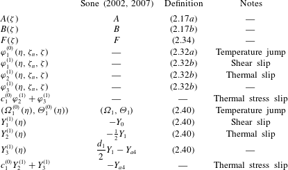
Table 1. The numerical values of slip/jump coefficients under the diffuse reflection boundary condition for an HS gas and for the BGK model (Sone Reference Sone2002, Reference Sone2007; Takata & Hattori Reference Takata and Hattori2012). The correspondence to the notations in Sone (Reference Sone2002, Reference Sone2007) are also shown.

Finally, we present the Knudsen-layer correction for the macroscopic variables. Corresponding to (2.19), the macroscopic quantities
 $h$
(
$h$
(
 $h=\unicode[STIX]{x1D714},u_{i},\unicode[STIX]{x1D70F},P$
) are expressed as
$h=\unicode[STIX]{x1D714},u_{i},\unicode[STIX]{x1D70F},P$
) are expressed as
 $h=h_{H}+h_{K}$
, where
$h=h_{H}+h_{K}$
, where
 $h_{K}$
is given by (2.4) with
$h_{K}$
is given by (2.4) with
 $h=h_{K}$
and
$h=h_{K}$
and
 $\unicode[STIX]{x1D719}=\unicode[STIX]{x1D719}_{K}$
. Corresponding to the expansion of
$\unicode[STIX]{x1D719}=\unicode[STIX]{x1D719}_{K}$
. Corresponding to the expansion of
 $\unicode[STIX]{x1D719}_{K}$
in
$\unicode[STIX]{x1D719}_{K}$
in
 $\unicode[STIX]{x1D700}$
, we have
$\unicode[STIX]{x1D700}$
, we have
 $$\begin{eqnarray}h_{K}=h_{K1}\unicode[STIX]{x1D700}+h_{K2}\unicode[STIX]{x1D700}^{2}+\cdots \,,\end{eqnarray}$$
with
 $$\begin{eqnarray}\displaystyle & \unicode[STIX]{x1D714}_{Km}=\langle \unicode[STIX]{x1D719}_{Km}\rangle ,\quad u_{iKm}=\langle \unicode[STIX]{x1D701}_{i}\unicode[STIX]{x1D719}_{Km}\rangle , & \displaystyle\end{eqnarray}$$
 $$\begin{eqnarray}\displaystyle & \unicode[STIX]{x1D70F}_{Km}={\textstyle \frac{2}{3}}\langle (\unicode[STIX]{x1D701}_{j}^{2}-{\textstyle \frac{3}{2}})\unicode[STIX]{x1D719}_{Km}\rangle ,\quad P_{Km}={\textstyle \frac{2}{3}}\langle \unicode[STIX]{x1D701}_{j}^{2}\unicode[STIX]{x1D719}_{Km}\rangle , & \displaystyle\end{eqnarray}$$
 $m=1,2,\ldots$
). Since
$m=1,2,\ldots$
). Since
 $\unicode[STIX]{x1D719}_{K1}$
is expressed by (2.30), the direct substitution into (2.38) yields the following expressions for the macroscopic quantities in the Knudsen layer:
$\unicode[STIX]{x1D719}_{K1}$
is expressed by (2.30), the direct substitution into (2.38) yields the following expressions for the macroscopic quantities in the Knudsen layer:  $$\begin{eqnarray}\displaystyle & \unicode[STIX]{x1D714}_{K1}=\unicode[STIX]{x1D6FA}_{1}^{(0)}n_{i}(\unicode[STIX]{x2202}_{i}\unicode[STIX]{x1D70F}_{H0})_{0},\quad \unicode[STIX]{x1D70F}_{K1}=\unicode[STIX]{x1D6E9}_{1}^{(0)}n_{i}(\unicode[STIX]{x2202}_{i}\unicode[STIX]{x1D70F}_{H0})_{0}, & \displaystyle\end{eqnarray}$$
 $$\begin{eqnarray}\displaystyle & P_{K1}=(\unicode[STIX]{x1D6FA}_{1}^{(0)}+\unicode[STIX]{x1D6E9}_{1}^{(0)})n_{i}(\unicode[STIX]{x2202}_{i}\unicode[STIX]{x1D70F}_{H0})_{0}=\unicode[STIX]{x1D714}_{K1}+\unicode[STIX]{x1D70F}_{K1}, & \displaystyle\end{eqnarray}$$
 $$\begin{eqnarray}\displaystyle & u_{iK1}n_{i}=0,\quad u_{iK1}t_{i}=Y_{1}^{(1)}t_{i}n_{j}(\unicode[STIX]{x2202}_{j}u_{iH0}+\unicode[STIX]{x2202}_{i}u_{jH0})_{0}+Y_{2}^{(1)}t_{i}(\unicode[STIX]{x2202}_{i}\unicode[STIX]{x1D70F}_{H0})_{0}, & \displaystyle\end{eqnarray}$$
 $\unicode[STIX]{x1D6FA}_{1}^{(0)}=\unicode[STIX]{x1D6FA}_{1}^{(0)}(\unicode[STIX]{x1D702})$
,
$\unicode[STIX]{x1D6FA}_{1}^{(0)}=\unicode[STIX]{x1D6FA}_{1}^{(0)}(\unicode[STIX]{x1D702})$
,
 $\unicode[STIX]{x1D6E9}_{1}^{(0)}=\unicode[STIX]{x1D6E9}_{1}^{(0)}(\unicode[STIX]{x1D702})$
, and
$\unicode[STIX]{x1D6E9}_{1}^{(0)}=\unicode[STIX]{x1D6E9}_{1}^{(0)}(\unicode[STIX]{x1D702})$
, and
 $Y_{j}^{(1)}=Y_{j}^{(1)}(\unicode[STIX]{x1D702})$
are defined by
$Y_{j}^{(1)}=Y_{j}^{(1)}(\unicode[STIX]{x1D702})$
are defined by  $$\begin{eqnarray}\unicode[STIX]{x1D6FA}_{1}^{(0)}=\langle \unicode[STIX]{x1D711}_{1}^{(0)}\rangle ,\quad \unicode[STIX]{x1D6E9}_{1}^{(0)}={\textstyle \frac{2}{3}}\langle (\unicode[STIX]{x1D701}^{2}-{\textstyle \frac{3}{2}})\unicode[STIX]{x1D711}_{1}^{(0)}\rangle ,\quad Y_{j}^{(1)}={\textstyle \frac{1}{2}}\langle (\unicode[STIX]{x1D701}^{2}-\unicode[STIX]{x1D701}_{n}^{2})\unicode[STIX]{x1D711}_{j}^{(1)}\rangle .\end{eqnarray}$$
Note that
 $\langle \unicode[STIX]{x1D701}_{n}\unicode[STIX]{x1D711}_{1}^{(0)}\rangle =0$
was used in the derivation of (2.39).
$\langle \unicode[STIX]{x1D701}_{n}\unicode[STIX]{x1D711}_{1}^{(0)}\rangle =0$
was used in the derivation of (2.39).
2.4 Summary of Sone’s asymptotics
In this section, we have considered the steady behaviour of a rarefied gas between two parallel plates whose temperature distribution is a smooth function of
 $x_{2}$
and
$x_{2}$
and
 $x_{3}$
in the case where the Knudsen number is small. Its velocity distribution functions are expressed as
$x_{3}$
in the case where the Knudsen number is small. Its velocity distribution functions are expressed as
 $$\begin{eqnarray}\unicode[STIX]{x1D719}=\unicode[STIX]{x1D719}_{H0}+\unicode[STIX]{x1D700}(\unicode[STIX]{x1D719}_{H1}+\unicode[STIX]{x1D719}_{K1})+\cdots \,,\end{eqnarray}$$
with
 $$\begin{eqnarray}\unicode[STIX]{x1D719}_{H0}=\unicode[STIX]{x1D719}_{eH0},\end{eqnarray}$$
 $$\begin{eqnarray}\unicode[STIX]{x1D719}_{H1}=\unicode[STIX]{x1D719}_{eH1}-\unicode[STIX]{x1D701}_{i}A(\unicode[STIX]{x1D701})\unicode[STIX]{x2202}_{i}\unicode[STIX]{x1D70F}_{H0}-{\textstyle \frac{1}{2}}\unicode[STIX]{x1D701}_{i}\unicode[STIX]{x1D701}_{j}B(\unicode[STIX]{x1D701})(\unicode[STIX]{x2202}_{i}u_{jH0}+\unicode[STIX]{x2202}_{j}u_{iH0}),\end{eqnarray}$$
 $$\begin{eqnarray}\displaystyle \unicode[STIX]{x1D719}_{K1} & = & \displaystyle \unicode[STIX]{x1D711}_{1}^{(0)}(\unicode[STIX]{x1D702},\unicode[STIX]{x1D701}_{n},\unicode[STIX]{x1D701})n_{i}(\unicode[STIX]{x2202}_{i}\unicode[STIX]{x1D70F}_{H0})_{0}\nonumber\\ \displaystyle & & \displaystyle +\,\overline{\unicode[STIX]{x1D701}}_{i}\unicode[STIX]{x1D711}_{1}^{(1)}(\unicode[STIX]{x1D702},\unicode[STIX]{x1D701}_{n},\unicode[STIX]{x1D701})n_{j}(\unicode[STIX]{x2202}_{j}u_{iH0}+\unicode[STIX]{x2202}_{i}u_{jH0})_{0}+\overline{\unicode[STIX]{x1D701}}_{i}\unicode[STIX]{x1D711}_{2}^{(1)}(\unicode[STIX]{x1D702},\unicode[STIX]{x1D701}_{n},\unicode[STIX]{x1D701})(\unicode[STIX]{x2202}_{i}\unicode[STIX]{x1D70F}_{H0})_{0},\end{eqnarray}$$
 $\unicode[STIX]{x1D719}_{eHm}$
is given by (2.16). In these expressions,
$\unicode[STIX]{x1D719}_{eHm}$
is given by (2.16). In these expressions,
 $A$
,
$A$
,
 $B$
,
$B$
,
 $\unicode[STIX]{x1D711}_{1}^{(0)}$
, and
$\unicode[STIX]{x1D711}_{1}^{(0)}$
, and
 $\unicode[STIX]{x1D711}_{j}^{(1)}$
are universal in the sense that they do not depend on specific problems. On the other hand, the macroscopic variables arising in the velocity distribution functions contain the specific information of the problem under consideration. They are obtained by solving the Stokes system (2.11)–(2.12) under the following boundary conditions on
$\unicode[STIX]{x1D711}_{j}^{(1)}$
are universal in the sense that they do not depend on specific problems. On the other hand, the macroscopic variables arising in the velocity distribution functions contain the specific information of the problem under consideration. They are obtained by solving the Stokes system (2.11)–(2.12) under the following boundary conditions on
 $x_{1}=\mp a$
:
$x_{1}=\mp a$
:-
(1) order
$\unicode[STIX]{x1D700}^{0}$
(2.44)
$$\begin{eqnarray}u_{iH0}=0,\quad \unicode[STIX]{x1D70F}_{H0}=\unicode[STIX]{x1D70F}_{w}(x_{2},x_{3}),\end{eqnarray}$$
-
(2) order
$\unicode[STIX]{x1D700}^{1}$
(2.45a )
$$\begin{eqnarray}\displaystyle & \unicode[STIX]{x1D70F}_{H1}=c_{1}^{(0)}n_{i}\unicode[STIX]{x2202}_{i}\unicode[STIX]{x1D70F}_{H0}, & \displaystyle\end{eqnarray}$$
(2.45b )
$$\begin{eqnarray}\displaystyle & u_{1H1}=0, & \displaystyle\end{eqnarray}$$
(2.45c )
$$\begin{eqnarray}\displaystyle & u_{iH1}t_{i}=b_{1}^{(1)}t_{i}n_{j}(\unicode[STIX]{x2202}_{j}u_{iH0}+\unicode[STIX]{x2202}_{i}u_{jH0})+b_{2}^{(1)}t_{i}\unicode[STIX]{x2202}_{i}\unicode[STIX]{x1D70F}_{H0}. & \displaystyle\end{eqnarray}$$


The formulae for the Knudsen-layer corrections are summarized in (2.39). Table 2 summarizes the universal functions.
Table 2. List of universal functions. The correspondence to the notations in Sone (Reference Sone2002, Reference Sone2007) are also shown.
3 Behaviour of a slightly rarefied gas between two parallel plates with a discontinuous surface temperature
In this section, we discuss the case of a discontinuous surface temperature based on the result obtained in the previous section. Let us denote again by
 $L$
the reference length, by
$L$
the reference length, by
 $\unicode[STIX]{x1D70C}_{0}$
the reference density, by
$\unicode[STIX]{x1D70C}_{0}$
the reference density, by
 $T_{0}$
the reference temperature, and by
$T_{0}$
the reference temperature, and by
 $p_{0}=\unicode[STIX]{x1D70C}_{0}RT_{0}$
the reference pressure, and consider the following problem.
$p_{0}=\unicode[STIX]{x1D70C}_{0}RT_{0}$
the reference pressure, and consider the following problem.
3.1 Problem
Consider a rarefied gas confined between two parallel plates located at
 $x_{1}=\pm \unicode[STIX]{x03C0}/2$
, where
$x_{1}=\pm \unicode[STIX]{x03C0}/2$
, where
 $Lx_{i}$
is the space rectangular coordinate system (figure 1). The two plates are heated (or cooled) non-uniformly in the following way. That is, the upper halves
$Lx_{i}$
is the space rectangular coordinate system (figure 1). The two plates are heated (or cooled) non-uniformly in the following way. That is, the upper halves
 $(x_{2}>0)$
are kept at a uniform temperature
$(x_{2}>0)$
are kept at a uniform temperature
 $T_{0}(1+\unicode[STIX]{x1D70F}_{w})$
, while the lower halves (
$T_{0}(1+\unicode[STIX]{x1D70F}_{w})$
, while the lower halves (
 $x_{2}<0$
) are kept at another uniform temperature
$x_{2}<0$
) are kept at another uniform temperature
 $T_{0}(1-\unicode[STIX]{x1D70F}_{w})$
, where
$T_{0}(1-\unicode[STIX]{x1D70F}_{w})$
, where
 $\unicode[STIX]{x1D70F}_{w}$
is a constant. Thus, the surface temperature of the channel is discontinuous at
$\unicode[STIX]{x1D70F}_{w}$
is a constant. Thus, the surface temperature of the channel is discontinuous at
 $x_{2}=0$
with jump
$x_{2}=0$
with jump
 $2T_{0}|\unicode[STIX]{x1D70F}_{w}|$
. There is no pressure gradient imposed on the gas nor external force. We investigate the steady behaviour of the gas in the channel on the basis of the Boltzmann equation and the diffuse reflection boundary condition, under the assumption that
$2T_{0}|\unicode[STIX]{x1D70F}_{w}|$
. There is no pressure gradient imposed on the gas nor external force. We investigate the steady behaviour of the gas in the channel on the basis of the Boltzmann equation and the diffuse reflection boundary condition, under the assumption that
 $|\unicode[STIX]{x1D70F}_{w}|$
is so small that the equation and boundary conditions can be linearized around the reference equilibrium state at rest. In particular, we pay special attention to the behaviour of the gas when the Knudsen number
$|\unicode[STIX]{x1D70F}_{w}|$
is so small that the equation and boundary conditions can be linearized around the reference equilibrium state at rest. In particular, we pay special attention to the behaviour of the gas when the Knudsen number
 $Kn=\ell _{0}/L$
, or
$Kn=\ell _{0}/L$
, or
 $\unicode[STIX]{x1D700}=(\sqrt{\unicode[STIX]{x03C0}}/2)Kn$
, is small, where
$\unicode[STIX]{x1D700}=(\sqrt{\unicode[STIX]{x03C0}}/2)Kn$
, is small, where
 $\ell _{0}$
is the mean free path of the gas molecules in the equilibrium state at rest with temperature
$\ell _{0}$
is the mean free path of the gas molecules in the equilibrium state at rest with temperature
 $T_{0}$
and density
$T_{0}$
and density
 $\unicode[STIX]{x1D70C}_{0}$
.
$\unicode[STIX]{x1D70C}_{0}$
.

Figure 1. Problem.
We use the same notations as in the previous section. That is, the velocity distribution function is denoted by
 $\unicode[STIX]{x1D70C}_{0}(2RT_{0})^{-3/2}(1+\unicode[STIX]{x1D719}(x_{1},x_{2},\unicode[STIX]{x1D701}_{i}))E$
. Here, we have assumed that the state of the gas is independent of
$\unicode[STIX]{x1D70C}_{0}(2RT_{0})^{-3/2}(1+\unicode[STIX]{x1D719}(x_{1},x_{2},\unicode[STIX]{x1D701}_{i}))E$
. Here, we have assumed that the state of the gas is independent of
 $x_{3}$
. Then,
$x_{3}$
. Then,
 $\unicode[STIX]{x1D719}$
satisfies the following equation and boundary conditions:
$\unicode[STIX]{x1D719}$
satisfies the following equation and boundary conditions:
 $$\begin{eqnarray}\displaystyle & \displaystyle \unicode[STIX]{x1D701}_{1}\unicode[STIX]{x2202}_{1}\unicode[STIX]{x1D719}+\unicode[STIX]{x1D701}_{2}\unicode[STIX]{x2202}_{2}\unicode[STIX]{x1D719}=\frac{1}{\unicode[STIX]{x1D700}}{\mathcal{L}}(\unicode[STIX]{x1D719}),\quad \left(-\frac{\unicode[STIX]{x03C0}}{2}<x_{1}<\frac{\unicode[STIX]{x03C0}}{2},-\infty <x_{2}<\infty \right), & \displaystyle\end{eqnarray}$$
 $$\begin{eqnarray}\displaystyle & \displaystyle \unicode[STIX]{x1D719}=2\sqrt{\unicode[STIX]{x03C0}}\int _{\unicode[STIX]{x1D701}_{1}<0}|\unicode[STIX]{x1D701}_{1}|\unicode[STIX]{x1D719}E\,\text{d}\unicode[STIX]{x1D73B}\pm (\unicode[STIX]{x1D701}_{j}^{2}-2)\unicode[STIX]{x1D70F}_{w},\quad \unicode[STIX]{x1D701}_{1}>0,\quad \left(x_{1}=-\frac{\unicode[STIX]{x03C0}}{2},~x_{2}\gtrless 0\right), & \displaystyle\end{eqnarray}$$
 $$\begin{eqnarray}\displaystyle & \displaystyle \unicode[STIX]{x1D719}=2\sqrt{\unicode[STIX]{x03C0}}\int _{\unicode[STIX]{x1D701}_{1}>0}|\unicode[STIX]{x1D701}_{1}|\unicode[STIX]{x1D719}E\,\text{d}\unicode[STIX]{x1D73B}\pm (\unicode[STIX]{x1D701}_{j}^{2}-2)\unicode[STIX]{x1D70F}_{w},\quad \unicode[STIX]{x1D701}_{1}<0,\quad \left(x_{1}=\frac{\unicode[STIX]{x03C0}}{2},~x_{2}\gtrless 0\right). & \displaystyle\end{eqnarray}$$
The macroscopic variables, the density
 $\unicode[STIX]{x1D70C}_{0}(1+\unicode[STIX]{x1D714})$
, the flow velocity
$\unicode[STIX]{x1D70C}_{0}(1+\unicode[STIX]{x1D714})$
, the flow velocity
 $(2RT_{0})^{1/2}u_{i}$
(
$(2RT_{0})^{1/2}u_{i}$
(
 $u_{3}=0$
), the temperature
$u_{3}=0$
), the temperature
 $T_{0}(1+\unicode[STIX]{x1D70F})$
, and the pressure
$T_{0}(1+\unicode[STIX]{x1D70F})$
, and the pressure
 $p_{0}(1+P)$
, are defined as before, and we do not repeat it here (see (2.4)). Note that they are functions of
$p_{0}(1+P)$
, are defined as before, and we do not repeat it here (see (2.4)). Note that they are functions of
 $(x_{1},x_{2})$
in the present section.
$(x_{1},x_{2})$
in the present section.
We observe that a solution that is even in
 $(x_{1},\unicode[STIX]{x1D701}_{1})$
and odd (antisymmetric) in
$(x_{1},\unicode[STIX]{x1D701}_{1})$
and odd (antisymmetric) in
 $(x_{2},\unicode[STIX]{x1D701}_{2})$
is compatible with the present problem, i.e.
$(x_{2},\unicode[STIX]{x1D701}_{2})$
is compatible with the present problem, i.e.
 $$\begin{eqnarray}\displaystyle & \displaystyle \unicode[STIX]{x1D719}(-x_{1},x_{2},-\unicode[STIX]{x1D701}_{1},\unicode[STIX]{x1D701}_{2},\unicode[STIX]{x1D701}_{3})=\unicode[STIX]{x1D719}(x_{1},x_{2},\unicode[STIX]{x1D701}_{1},\unicode[STIX]{x1D701}_{2},\unicode[STIX]{x1D701}_{3}), & \displaystyle\end{eqnarray}$$
 $$\begin{eqnarray}\displaystyle & \displaystyle \unicode[STIX]{x1D719}(x_{1},-x_{2},\unicode[STIX]{x1D701}_{1},-\unicode[STIX]{x1D701}_{2},\unicode[STIX]{x1D701}_{3})=-\unicode[STIX]{x1D719}(x_{1},x_{2},\unicode[STIX]{x1D701}_{1},\unicode[STIX]{x1D701}_{2},\unicode[STIX]{x1D701}_{3}). & \displaystyle\end{eqnarray}$$
 $x_{2}>0$
by imposing the following reflection condition at
$x_{2}>0$
by imposing the following reflection condition at
 $x_{2}=0$
:
$x_{2}=0$
:  $$\begin{eqnarray}\unicode[STIX]{x1D719}(x_{1},0,\unicode[STIX]{x1D701}_{1},\unicode[STIX]{x1D701}_{2},\unicode[STIX]{x1D701}_{3})=-\unicode[STIX]{x1D719}(x_{1},0,\unicode[STIX]{x1D701}_{1},-\unicode[STIX]{x1D701}_{2},\unicode[STIX]{x1D701}_{3}),\quad \unicode[STIX]{x1D701}_{2}>0.\end{eqnarray}$$
In what follows, we denote the restriction of
 $\unicode[STIX]{x1D719}$
to
$\unicode[STIX]{x1D719}$
to
 $x_{2}\gtrless 0$
by
$x_{2}\gtrless 0$
by
 $\unicode[STIX]{x1D719}^{\pm }$
and we shall mainly consider
$\unicode[STIX]{x1D719}^{\pm }$
and we shall mainly consider
 $\unicode[STIX]{x1D719}^{+}$
in the sequel. Likewise,
$\unicode[STIX]{x1D719}^{+}$
in the sequel. Likewise,
 $h^{\pm }$
(
$h^{\pm }$
(
 $h=\unicode[STIX]{x1D714},u_{i},\unicode[STIX]{x1D70F}$
and
$h=\unicode[STIX]{x1D714},u_{i},\unicode[STIX]{x1D70F}$
and
 $P$
) denotes the restriction of
$P$
) denotes the restriction of
 $h$
to
$h$
to
 $x_{2}\gtrless 0$
. Once
$x_{2}\gtrless 0$
. Once
 $\unicode[STIX]{x1D719}^{+}$
is obtained,
$\unicode[STIX]{x1D719}^{+}$
is obtained,
 $\unicode[STIX]{x1D719}^{-}$
is readily obtained by the relation
$\unicode[STIX]{x1D719}^{-}$
is readily obtained by the relation
 $\unicode[STIX]{x1D719}^{-}(x_{1},x_{2},\unicode[STIX]{x1D701}_{1},\unicode[STIX]{x1D701}_{2},\unicode[STIX]{x1D701}_{3})=-\unicode[STIX]{x1D719}^{+}(x_{1},-x_{2},\unicode[STIX]{x1D701}_{1},-\unicode[STIX]{x1D701}_{2},\unicode[STIX]{x1D701}_{3})$
.
$\unicode[STIX]{x1D719}^{-}(x_{1},x_{2},\unicode[STIX]{x1D701}_{1},\unicode[STIX]{x1D701}_{2},\unicode[STIX]{x1D701}_{3})=-\unicode[STIX]{x1D719}^{+}(x_{1},-x_{2},\unicode[STIX]{x1D701}_{1},-\unicode[STIX]{x1D701}_{2},\unicode[STIX]{x1D701}_{3})$
.
3.2 Asymptotic matching
We try to investigate the boundary-value problem for
 $\unicode[STIX]{x1D719}^{+}$
for small
$\unicode[STIX]{x1D719}^{+}$
for small
 $\unicode[STIX]{x1D700}\ll 1$
. The idea is to apply the method of matched asymptotic expansion (Dyke Reference Dyke1975; Taguchi Reference Taguchi2015; Taguchi & Suzuki Reference Taguchi and Suzuki2017) by regarding Sone’s asymptotic solution as the outer solution. More precisely, we use the result derived in § 2 to construct the overall solution in the upper-half domain, which is possible because the temperature of the boundary is uniform. The effect of the discontinuous surface temperature is then transferred to the mismatch of the diffuse reflection conditions (3.2) and (3.3) on
$\unicode[STIX]{x1D700}\ll 1$
. The idea is to apply the method of matched asymptotic expansion (Dyke Reference Dyke1975; Taguchi Reference Taguchi2015; Taguchi & Suzuki Reference Taguchi and Suzuki2017) by regarding Sone’s asymptotic solution as the outer solution. More precisely, we use the result derived in § 2 to construct the overall solution in the upper-half domain, which is possible because the temperature of the boundary is uniform. The effect of the discontinuous surface temperature is then transferred to the mismatch of the diffuse reflection conditions (3.2) and (3.3) on
 $x_{1}=\mp \unicode[STIX]{x03C0}/2$
and
$x_{1}=\mp \unicode[STIX]{x03C0}/2$
and
 $x_{2}>0$
and the reflection condition (3.5) on
$x_{2}>0$
and the reflection condition (3.5) on
 $x_{2}=0$
and
$x_{2}=0$
and
 $-\unicode[STIX]{x03C0}/2<x_{1}<\unicode[STIX]{x03C0}/2$
at the corners
$-\unicode[STIX]{x03C0}/2<x_{1}<\unicode[STIX]{x03C0}/2$
at the corners
 $(x_{1},x_{2})=(\mp \unicode[STIX]{x03C0}/2,0)$
. This mismatch causes an abrupt spatial variation of the solution in the vicinity of the corner, which Sone’s asymptotic solution cannot describe. Thus, we require an internal layer in the vicinity of the corner to alter the Sone’s asymptotic solution in a suitable way. The introduction of this new layer (different from the Knudsen layer) is the key ingredient of the present analysis.
$(x_{1},x_{2})=(\mp \unicode[STIX]{x03C0}/2,0)$
. This mismatch causes an abrupt spatial variation of the solution in the vicinity of the corner, which Sone’s asymptotic solution cannot describe. Thus, we require an internal layer in the vicinity of the corner to alter the Sone’s asymptotic solution in a suitable way. The introduction of this new layer (different from the Knudsen layer) is the key ingredient of the present analysis.
In this paper, we shall carry out the asymptotic analysis to the first order of
 $\unicode[STIX]{x1D700}$
.
$\unicode[STIX]{x1D700}$
.
3.2.1 Outer solution: zeroth order in
$\unicode[STIX]{x1D700}$

Let us consider the overall solution in the channel, which is intended to describe the behaviour of the gas except in the region close to the point of the surface temperature discontinuity. This solution is assumed to have the length scale of variation of the order of unity except in a thin layer adjacent to the boundary (the Knudsen layer), where the solution is allowed to change abruptly in the direction normal to the boundary. We call this solution the outer solution and denote it by attaching the subscript
 $F$
as
$F$
as
 $\unicode[STIX]{x1D719}_{F}$
(or
$\unicode[STIX]{x1D719}_{F}$
(or
 $\unicode[STIX]{x1D719}_{F}^{\pm }$
). In this section, we obtain the zeroth-order (leading-order) approximation of the outer solution
$\unicode[STIX]{x1D719}_{F}^{\pm }$
). In this section, we obtain the zeroth-order (leading-order) approximation of the outer solution
 $\unicode[STIX]{x1D719}_{F}^{+}$
.
$\unicode[STIX]{x1D719}_{F}^{+}$
.
First, putting aside the potential difficulty which may arise near the discontinuity points, we express
 $\unicode[STIX]{x1D719}_{F}^{+}$
as the combination of the Hilbert solution
$\unicode[STIX]{x1D719}_{F}^{+}$
as the combination of the Hilbert solution
 $\unicode[STIX]{x1D719}_{H}^{+}$
and the Knudsen-layer correction
$\unicode[STIX]{x1D719}_{H}^{+}$
and the Knudsen-layer correction
 $\unicode[STIX]{x1D719}_{K}^{+}$
:
$\unicode[STIX]{x1D719}_{K}^{+}$
:
 $$\begin{eqnarray}\unicode[STIX]{x1D719}_{F}^{+}=\unicode[STIX]{x1D719}_{H}^{+}+\unicode[STIX]{x1D719}_{K}^{+}.\end{eqnarray}$$
The length scale of variation of the Hilbert solution is of the order of unity, whereas the Knudsen-layer correction, which is appreciable only in a thin layer adjacent to the boundary, has the length scale of variation of the order of
 $\unicode[STIX]{x1D700}$
in the direction normal to the boundary (i.e.
$\unicode[STIX]{x1D700}$
in the direction normal to the boundary (i.e.
 $\unicode[STIX]{x2202}_{i}\unicode[STIX]{x1D719}_{H}=O(\unicode[STIX]{x1D719}_{H})$
,
$\unicode[STIX]{x2202}_{i}\unicode[STIX]{x1D719}_{H}=O(\unicode[STIX]{x1D719}_{H})$
,
 $\unicode[STIX]{x2202}_{1}\unicode[STIX]{x1D719}_{K}=O(\unicode[STIX]{x1D719}_{K}/\unicode[STIX]{x1D700})$
and
$\unicode[STIX]{x2202}_{1}\unicode[STIX]{x1D719}_{K}=O(\unicode[STIX]{x1D719}_{K}/\unicode[STIX]{x1D700})$
and
 $\unicode[STIX]{x2202}_{2}\unicode[STIX]{x1D719}_{K}=O(\unicode[STIX]{x1D719}_{K})$
). According to § 2,
$\unicode[STIX]{x2202}_{2}\unicode[STIX]{x1D719}_{K}=O(\unicode[STIX]{x1D719}_{K})$
). According to § 2,
 $\unicode[STIX]{x1D719}_{H}^{+}$
and
$\unicode[STIX]{x1D719}_{H}^{+}$
and
 $\unicode[STIX]{x1D719}_{K}^{+}$
are expanded in
$\unicode[STIX]{x1D719}_{K}^{+}$
are expanded in
 $\unicode[STIX]{x1D700}$
as
$\unicode[STIX]{x1D700}$
as
 $$\begin{eqnarray}\displaystyle & \unicode[STIX]{x1D719}_{H}^{+}=\unicode[STIX]{x1D719}_{H0}^{+}+\unicode[STIX]{x1D700}\unicode[STIX]{x1D719}_{H1}^{+}+\cdots \,, & \displaystyle\end{eqnarray}$$
 $$\begin{eqnarray}\displaystyle & \unicode[STIX]{x1D719}_{K}^{+}=\unicode[STIX]{x1D700}\unicode[STIX]{x1D719}_{K1}^{+}+\cdots \,. & \displaystyle\end{eqnarray}$$
 $\unicode[STIX]{x1D719}_{F}^{+}$
in
$\unicode[STIX]{x1D719}_{F}^{+}$
in
 $\unicode[STIX]{x1D700}$
in the form
$\unicode[STIX]{x1D700}$
in the form  $$\begin{eqnarray}\unicode[STIX]{x1D719}_{F}^{+}=\unicode[STIX]{x1D719}_{F0}^{+}+\unicode[STIX]{x1D700}\unicode[STIX]{x1D719}_{F1}^{+}+\cdots \,,\end{eqnarray}$$
where
 $$\begin{eqnarray}\displaystyle & \unicode[STIX]{x1D719}_{F0}^{+}=\unicode[STIX]{x1D719}_{H0}^{+}, & \displaystyle\end{eqnarray}$$
 $$\begin{eqnarray}\displaystyle & \unicode[STIX]{x1D719}_{F1}^{+}=\unicode[STIX]{x1D719}_{H1}^{+}+\unicode[STIX]{x1D719}_{K1}^{+}. & \displaystyle\end{eqnarray}$$
 $\unicode[STIX]{x1D719}_{F}^{+}$
, the macroscopic quantities are also expanded in
$\unicode[STIX]{x1D719}_{F}^{+}$
, the macroscopic quantities are also expanded in
 $\unicode[STIX]{x1D700}$
as
$\unicode[STIX]{x1D700}$
as  $$\begin{eqnarray}h_{F}^{+}=h_{F0}^{+}+\unicode[STIX]{x1D700}h_{F1}^{+}+\cdots \,,\quad (h=\unicode[STIX]{x1D714},u_{i},\unicode[STIX]{x1D70F},P),\end{eqnarray}$$
where
 $$\begin{eqnarray}\displaystyle & h_{F0}^{+}=h_{H0}^{+}, & \displaystyle\end{eqnarray}$$
 $$\begin{eqnarray}\displaystyle & h_{F1}^{+}=h_{H1}^{+}+h_{K1}^{+}. & \displaystyle\end{eqnarray}$$
 $h_{Hm}^{+}$
and
$h_{Hm}^{+}$
and
 $\unicode[STIX]{x1D719}_{Hm}^{+}$
and that between
$\unicode[STIX]{x1D719}_{Hm}^{+}$
and that between
 $h_{Km}^{+}$
and
$h_{Km}^{+}$
and
 $\unicode[STIX]{x1D719}_{Km}^{+}$
are given by (2.8) and (2.38) with
$\unicode[STIX]{x1D719}_{Km}^{+}$
are given by (2.8) and (2.38) with
 $(\unicode[STIX]{x1D719}_{Hm},h_{Hm})=(\unicode[STIX]{x1D719}_{Hm}^{+},h_{Hm}^{+})$
and
$(\unicode[STIX]{x1D719}_{Hm},h_{Hm})=(\unicode[STIX]{x1D719}_{Hm}^{+},h_{Hm}^{+})$
and
 $(\unicode[STIX]{x1D719}_{Km},h_{Km})=(\unicode[STIX]{x1D719}_{Km}^{+},h_{Km}^{+})$
, respectively.
$(\unicode[STIX]{x1D719}_{Km},h_{Km})=(\unicode[STIX]{x1D719}_{Km}^{+},h_{Km}^{+})$
, respectively.
From the result of § 2, the leading-order term of the outer solution
 $\unicode[STIX]{x1D719}_{F0}^{+}$
is given by the local Maxwellian,
$\unicode[STIX]{x1D719}_{F0}^{+}$
is given by the local Maxwellian,
 $$\begin{eqnarray}\unicode[STIX]{x1D719}_{F0}^{+}=\unicode[STIX]{x1D719}_{H0}^{+}=P_{H0}^{+}+2\unicode[STIX]{x1D701}_{1}u_{1H0}^{+}+2\unicode[STIX]{x1D701}_{2}u_{2H0}^{+}+(\unicode[STIX]{x1D701}_{j}^{2}-{\textstyle \frac{5}{2}})\unicode[STIX]{x1D70F}_{H0}^{+},\end{eqnarray}$$
where the macroscopic variables solve the following Stokes problem in
 $D^{+}=\{(x_{1},x_{2})\,|-\unicode[STIX]{x03C0}/2<x_{1}<\unicode[STIX]{x03C0}/2,\,x_{2}>0\}$
:
$D^{+}=\{(x_{1},x_{2})\,|-\unicode[STIX]{x03C0}/2<x_{1}<\unicode[STIX]{x03C0}/2,\,x_{2}>0\}$
:
 $$\begin{eqnarray}\displaystyle & \unicode[STIX]{x2202}_{i}P_{H0}^{+}=0, & \displaystyle\end{eqnarray}$$
 $$\begin{eqnarray}\displaystyle & \unicode[STIX]{x2202}_{i}u_{iH0}^{+}=0,\quad \unicode[STIX]{x1D6FE}_{1}\unicode[STIX]{x1D6FB}^{2}u_{iH0}^{+}-\unicode[STIX]{x2202}_{i}P_{H1}^{+}=0, & \displaystyle\end{eqnarray}$$
 $$\begin{eqnarray}\displaystyle & \unicode[STIX]{x1D6FB}^{2}\unicode[STIX]{x1D70F}_{H0}^{+}=0, & \displaystyle\end{eqnarray}$$
 $$\begin{eqnarray}\displaystyle & \displaystyle u_{iH0}^{+}=0,\quad \left(x_{1}=\mp \frac{\unicode[STIX]{x03C0}}{2},x_{2}>0\right), & \displaystyle\end{eqnarray}$$
 $$\begin{eqnarray}\displaystyle & \displaystyle \unicode[STIX]{x1D70F}_{H0}^{+}=\unicode[STIX]{x1D70F}_{w},\quad \left(x_{1}=\mp \frac{\unicode[STIX]{x03C0}}{2},x_{2}>0\right), & \displaystyle\end{eqnarray}$$
 $x_{2}=0$
, i.e.
$x_{2}=0$
, i.e.  $$\begin{eqnarray}P_{H0}^{+}=u_{1H0}^{+}=\unicode[STIX]{x1D70F}_{H0}^{+}=\unicode[STIX]{x2202}_{2}u_{2H0}^{+}=0,\quad \left(-\frac{\unicode[STIX]{x03C0}}{2}<x_{1}<\frac{\unicode[STIX]{x03C0}}{2},x_{2}=0\right)\end{eqnarray}$$
(see (3.5)). Here,
 $i\in \{1,2\}$
and
$i\in \{1,2\}$
and
 $\unicode[STIX]{x1D6FB}^{2}=\unicode[STIX]{x2202}_{1}^{2}+\unicode[STIX]{x2202}_{2}^{2}$
(the two-dimensional Laplacian). Equations (3.14a
) and (3.14b
) are the no-slip/no-jump conditions for the flow velocity and temperature, respectively (see (2.44)). Note that the density is determined from the temperature and pressure by the relation
$\unicode[STIX]{x1D6FB}^{2}=\unicode[STIX]{x2202}_{1}^{2}+\unicode[STIX]{x2202}_{2}^{2}$
(the two-dimensional Laplacian). Equations (3.14a
) and (3.14b
) are the no-slip/no-jump conditions for the flow velocity and temperature, respectively (see (2.44)). Note that the density is determined from the temperature and pressure by the relation
 $\unicode[STIX]{x1D714}_{H0}^{+}=P_{H0}^{+}-\unicode[STIX]{x1D70F}_{H0}^{+}$
.
$\unicode[STIX]{x1D714}_{H0}^{+}=P_{H0}^{+}-\unicode[STIX]{x1D70F}_{H0}^{+}$
.
First,
 $$\begin{eqnarray}P_{H0}^{+}=0\end{eqnarray}$$
trivially satisfies (3.13a ) and (3.15). Next, it is readily seen that
 $$\begin{eqnarray}u_{iH0}^{+}=0,\quad P_{H1}^{+}=0\end{eqnarray}$$
is also a trivial solution to the Stokes equations (3.13b
) that satisfies the boundary conditions (3.14a
) and (3.15). Note that
 $P_{H1}^{+}$
is only determined up to an additive constant from the Stokes equation. This constant, which should be determined from the information on the higher order, turns out to be zero if one considers the requirement (3.5). This result has already been used in (3.17). On the other hand,
$P_{H1}^{+}$
is only determined up to an additive constant from the Stokes equation. This constant, which should be determined from the information on the higher order, turns out to be zero if one considers the requirement (3.5). This result has already been used in (3.17). On the other hand,
 $\unicode[STIX]{x1D70F}_{H0}^{+}$
satisfying the Laplace equation (3.13c
) and the boundary conditions (3.14b
) and (3.15) is given by
$\unicode[STIX]{x1D70F}_{H0}^{+}$
satisfying the Laplace equation (3.13c
) and the boundary conditions (3.14b
) and (3.15) is given by
 $$\begin{eqnarray}\displaystyle & \displaystyle \unicode[STIX]{x1D70F}_{H0}^{+}=\frac{\unicode[STIX]{x1D70F}_{w}}{\unicode[STIX]{x03C0}}\text{Arg}\left(\frac{1+\sin z}{1-\sin z}\right), & \displaystyle\end{eqnarray}$$
 $$\begin{eqnarray}\displaystyle & \displaystyle z=x_{1}+\text{i}\,x_{2}, & \displaystyle\end{eqnarray}$$
 $\text{i}$
is the imaginary unit. To summarize, the leading-order term of the outer solution is obtained as
$\text{i}$
is the imaginary unit. To summarize, the leading-order term of the outer solution is obtained as  $$\begin{eqnarray}\unicode[STIX]{x1D719}_{F0}^{+}=\left(\unicode[STIX]{x1D701}_{j}^{2}-{\textstyle \frac{5}{2}}\right)\unicode[STIX]{x1D70F}_{H0}^{+},\end{eqnarray}$$
with
 $\unicode[STIX]{x1D70F}_{H0}^{+}$
given by (3.18).
$\unicode[STIX]{x1D70F}_{H0}^{+}$
given by (3.18).
We observe that
 $\unicode[STIX]{x1D70F}_{H0}^{+}$
takes different values depending on the way of approach to the point
$\unicode[STIX]{x1D70F}_{H0}^{+}$
takes different values depending on the way of approach to the point
 $(x_{1},x_{2})=(-\unicode[STIX]{x03C0}/2,0)$
or
$(x_{1},x_{2})=(-\unicode[STIX]{x03C0}/2,0)$
or
 $(\unicode[STIX]{x03C0}/2,0)$
. This is seen by introducing a local polar coordinate system
$(\unicode[STIX]{x03C0}/2,0)$
. This is seen by introducing a local polar coordinate system
 $(r,\unicode[STIX]{x1D703})$
centred at
$(r,\unicode[STIX]{x1D703})$
centred at
 $(x_{1},x_{2})=(\mp \unicode[STIX]{x03C0}/2,0)$
by
$(x_{1},x_{2})=(\mp \unicode[STIX]{x03C0}/2,0)$
by
 $$\begin{eqnarray}x_{1}=\mp \frac{\unicode[STIX]{x03C0}}{2}\pm r\cos \unicode[STIX]{x1D703},\quad x_{2}=r\sin \unicode[STIX]{x1D703},\quad \left(\text{near }(x_{1},x_{2})=\left(\mp \frac{\unicode[STIX]{x03C0}}{2},0\right)\right)\end{eqnarray}$$
(
 $0\leqslant \unicode[STIX]{x1D703}\leqslant \unicode[STIX]{x03C0}/2$
). Expanding
$0\leqslant \unicode[STIX]{x1D703}\leqslant \unicode[STIX]{x03C0}/2$
). Expanding
 $\unicode[STIX]{x1D70F}_{H0}^{+}$
near each of the discontinuity points in terms of small
$\unicode[STIX]{x1D70F}_{H0}^{+}$
near each of the discontinuity points in terms of small
 $r$
, we obtain
$r$
, we obtain
 $$\begin{eqnarray}\frac{\unicode[STIX]{x1D70F}_{H0}^{+}}{\unicode[STIX]{x1D70F}_{w}}=\frac{2}{\unicode[STIX]{x03C0}}\unicode[STIX]{x1D703}+\frac{r^{2}}{6\unicode[STIX]{x03C0}}\sin 2\unicode[STIX]{x1D703}+O(r^{4}),\quad (r\ll 1).\end{eqnarray}$$
This shows that the limiting value of
 $\unicode[STIX]{x1D70F}_{H0}^{+}$
and therefore that of
$\unicode[STIX]{x1D70F}_{H0}^{+}$
and therefore that of
 $\unicode[STIX]{x1D719}_{F0}^{+}$
as
$\unicode[STIX]{x1D719}_{F0}^{+}$
as
 $r{\searrow}0$
are not uniquely determined but depend on
$r{\searrow}0$
are not uniquely determined but depend on
 $\unicode[STIX]{x1D703}$
.
$\unicode[STIX]{x1D703}$
.
3.2.2 Outer solution: first order in
$\unicode[STIX]{x1D700}$

Next, we proceed to the first order in the expansion of the outer solution. Unlike the zeroth order,
 $\unicode[STIX]{x1D719}_{F1}^{+}$
is composed of the Hilbert part
$\unicode[STIX]{x1D719}_{F1}^{+}$
is composed of the Hilbert part
 $\unicode[STIX]{x1D719}_{H1}^{+}$
and the Knudsen-layer part
$\unicode[STIX]{x1D719}_{H1}^{+}$
and the Knudsen-layer part
 $\unicode[STIX]{x1D719}_{K1}^{+}$
(see (3.9b
)). More precisely, with (3.18) and (3.17) obtained above, (2.43) with
$\unicode[STIX]{x1D719}_{K1}^{+}$
(see (3.9b
)). More precisely, with (3.18) and (3.17) obtained above, (2.43) with
 $\unicode[STIX]{x2202}_{3}=u_{3H1}=0$
is computed to give
$\unicode[STIX]{x2202}_{3}=u_{3H1}=0$
is computed to give
 $$\begin{eqnarray}\displaystyle \unicode[STIX]{x1D719}_{H1}^{+} & = & \displaystyle 2\unicode[STIX]{x1D701}_{1}u_{1H1}^{+}+2\unicode[STIX]{x1D701}_{2}u_{2H1}^{+}+\left(\unicode[STIX]{x1D701}_{j}^{2}-\frac{5}{2}\right)\unicode[STIX]{x1D70F}_{H1}^{+}\nonumber\\ \displaystyle & & \displaystyle -\,\frac{4\unicode[STIX]{x1D70F}_{w}}{\unicode[STIX]{x03C0}}A(\unicode[STIX]{x1D701})\frac{\unicode[STIX]{x1D701}_{1}\sin x_{1}\sinh x_{2}+\unicode[STIX]{x1D701}_{2}\cos x_{1}\cosh x_{2}}{\cos (2x_{1})+\cosh (2x_{2})},\end{eqnarray}$$
 $$\begin{eqnarray}\displaystyle \unicode[STIX]{x1D719}_{K1}^{+}=-\frac{2\unicode[STIX]{x1D70F}_{w}}{\unicode[STIX]{x03C0}}\frac{1}{\sinh x_{2}}\left(\unicode[STIX]{x1D711}_{1}^{(0)}\left(\left|x_{1}+\unicode[STIX]{x03C0}/2\right|/\unicode[STIX]{x1D700},\unicode[STIX]{x1D701}_{1},\unicode[STIX]{x1D701}\right)+\unicode[STIX]{x1D711}_{1}^{(0)}\left(\left|x_{1}-\unicode[STIX]{x03C0}/2\right|/\unicode[STIX]{x1D700},-\unicode[STIX]{x1D701}_{1},\unicode[STIX]{x1D701}\right)\right), & & \displaystyle \nonumber\\ \displaystyle & & \displaystyle\end{eqnarray}$$
 $\unicode[STIX]{x1D701}=(\unicode[STIX]{x1D701}_{j}^{2})^{1/2}$
and
$\unicode[STIX]{x1D701}=(\unicode[STIX]{x1D701}_{j}^{2})^{1/2}$
and
 $A$
and
$A$
and
 $\unicode[STIX]{x1D711}_{1}^{(0)}$
are the functions defined in (2.17a
) and (2.32a
), respectively. Note that
$\unicode[STIX]{x1D711}_{1}^{(0)}$
are the functions defined in (2.17a
) and (2.32a
), respectively. Note that
 $\unicode[STIX]{x1D711}_{1}^{(0)}$
is meaningful only in the Knudsen layer. Therefore, there is no overlap of the two terms in (3.22b
). The quantities
$\unicode[STIX]{x1D711}_{1}^{(0)}$
is meaningful only in the Knudsen layer. Therefore, there is no overlap of the two terms in (3.22b
). The quantities
 $u_{iH1}^{+}=u_{iH1}^{+}(x_{1},x_{2})$
and
$u_{iH1}^{+}=u_{iH1}^{+}(x_{1},x_{2})$
and
 $\unicode[STIX]{x1D70F}_{H1}^{+}=\unicode[STIX]{x1D70F}_{H1}^{+}(x_{1},x_{2})$
contained in (3.22a
) are determined by solving the first-order Stokes problem. We will present the explicit form of the problem later (see (3.37)–(3.39)). For the moment, it suffices to mention that, on solving this problem, we simply obtain the following first-order macroscopic quantities with a trivial flow velocity:
$\unicode[STIX]{x1D70F}_{H1}^{+}=\unicode[STIX]{x1D70F}_{H1}^{+}(x_{1},x_{2})$
contained in (3.22a
) are determined by solving the first-order Stokes problem. We will present the explicit form of the problem later (see (3.37)–(3.39)). For the moment, it suffices to mention that, on solving this problem, we simply obtain the following first-order macroscopic quantities with a trivial flow velocity:  $$\begin{eqnarray}\displaystyle & \displaystyle \unicode[STIX]{x1D70F}_{H1}^{+}=-\unicode[STIX]{x1D714}_{H1}^{+}=-\frac{8\unicode[STIX]{x1D70F}_{w}c_{1}^{(0)}}{\unicode[STIX]{x03C0}^{2}}\frac{x_{2}\cos x_{1}\cosh x_{2}+x_{1}\sin x_{1}\sinh x_{2}}{\cos (2x_{1})+\cosh (2x_{2})}, & \displaystyle\end{eqnarray}$$
 $$\begin{eqnarray}\displaystyle & \displaystyle u_{1H1}^{+}=u_{2H1}^{+}=0,\quad P_{H2}^{+}=\text{const}. & \displaystyle\end{eqnarray}$$
 $u_{iH1}=0$
on the boundary, which results from (2.45) because
$u_{iH1}=0$
on the boundary, which results from (2.45) because
 $\unicode[STIX]{x1D70F}_{w}$
is constant and
$\unicode[STIX]{x1D70F}_{w}$
is constant and
 $u_{iH0}=0$
.
$u_{iH0}=0$
.
Of course, our interest is a non-trivial flow velocity and the above result needs to be modified in a suitable way. At this point, however, we simply examine how
 $\unicode[STIX]{x1D719}_{F1}^{+}$
thus obtained (denoted by
$\unicode[STIX]{x1D719}_{F1}^{+}$
thus obtained (denoted by
 $\unicode[STIX]{x1D719}_{F1\ast }^{+}$
) behaves near the points of discontinuity.
$\unicode[STIX]{x1D719}_{F1\ast }^{+}$
) behaves near the points of discontinuity.
Using again the local polar coordinates introduced in (3.20) as well as the corresponding circumferential molecular velocity
 $\unicode[STIX]{x1D701}_{\unicode[STIX]{x1D703}}=\mp \unicode[STIX]{x1D701}_{1}\sin \unicode[STIX]{x1D703}+\unicode[STIX]{x1D701}_{2}\cos \unicode[STIX]{x1D703}$
near
$\unicode[STIX]{x1D701}_{\unicode[STIX]{x1D703}}=\mp \unicode[STIX]{x1D701}_{1}\sin \unicode[STIX]{x1D703}+\unicode[STIX]{x1D701}_{2}\cos \unicode[STIX]{x1D703}$
near
 $(x_{1},x_{2})=(\mp \unicode[STIX]{x03C0}/2,0)$
, the essential terms of
$(x_{1},x_{2})=(\mp \unicode[STIX]{x03C0}/2,0)$
, the essential terms of
 $\unicode[STIX]{x1D719}_{F1\ast }^{+}=\unicode[STIX]{x1D719}_{H1}^{+}+\unicode[STIX]{x1D719}_{K1}^{+}$
(with (3.22) and (3.23)) in the vicinity of
$\unicode[STIX]{x1D719}_{F1\ast }^{+}=\unicode[STIX]{x1D719}_{H1}^{+}+\unicode[STIX]{x1D719}_{K1}^{+}$
(with (3.22) and (3.23)) in the vicinity of
 $(x_{1},x_{2})=(\mp \unicode[STIX]{x03C0}/2,0)$
takes the form
$(x_{1},x_{2})=(\mp \unicode[STIX]{x03C0}/2,0)$
takes the form
 $$\begin{eqnarray}\displaystyle \unicode[STIX]{x1D719}_{F1\ast }^{+} & \simeq & \displaystyle -\frac{2\unicode[STIX]{x1D70F}_{w}}{\unicode[STIX]{x03C0}}\left[\frac{c_{1}^{(0)}\sin \unicode[STIX]{x1D703}}{r}\left(\unicode[STIX]{x1D701}_{j}^{2}-\frac{5}{2}\right)+\frac{\unicode[STIX]{x1D701}_{\unicode[STIX]{x1D703}}}{r}A(\unicode[STIX]{x1D701})+\frac{1}{x_{2}}\unicode[STIX]{x1D711}_{1}^{(0)}\left(\left|x_{1}\pm \unicode[STIX]{x03C0}/2\right|/\unicode[STIX]{x1D700},\pm \unicode[STIX]{x1D701}_{1},\unicode[STIX]{x1D701}\right)\right]\nonumber\\ \displaystyle & & \displaystyle +\,O(r),\quad (r\ll 1).\end{eqnarray}$$
Thus,
 $|\unicode[STIX]{x1D719}_{F1\ast }^{+}|$
diverges with the rate
$|\unicode[STIX]{x1D719}_{F1\ast }^{+}|$
diverges with the rate
 $r^{-1}$
on approaching the points of discontinuity. In other words, the outer solution based on Sone’s asymptotic theory is valid only in the region
$r^{-1}$
on approaching the points of discontinuity. In other words, the outer solution based on Sone’s asymptotic theory is valid only in the region
 $r\gg \unicode[STIX]{x1D700}$
.
$r\gg \unicode[STIX]{x1D700}$
.
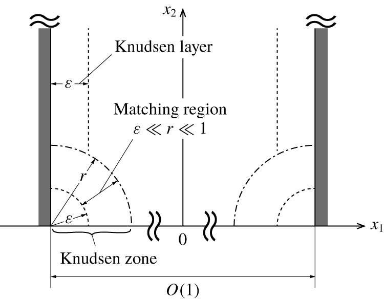
Figure 2. Schematics of the solution structure. Only the upper-half domain is shown.
3.2.3 Inner solution: zeroth order (leading order) in
$\unicode[STIX]{x1D700}$

We have seen that the outer solution breaks down in the vicinity of the point where the surface temperature has a jump. The reason is that the underlying length scale of variation of the Hilbert solution and that of the Knudsen-layer correction are too restrictive to describe the abrupt change that the flow undergoes near the points of discontinuity. This motivates us to introduce another inner layer near
 $(x_{1},x_{2})=(\mp \unicode[STIX]{x03C0}/2,0)$
, in which the solution is allowed to vary in
$(x_{1},x_{2})=(\mp \unicode[STIX]{x03C0}/2,0)$
, in which the solution is allowed to vary in
 $x_{1}$
and
$x_{1}$
and
 $x_{2}$
on the length scale of variation of the order of the (scaled) mean free path. This localized region near each of the discontinuity points may be called the Knudsen zone (see figure 2). Accordingly, the solution in this region is hereafter denoted by
$x_{2}$
on the length scale of variation of the order of the (scaled) mean free path. This localized region near each of the discontinuity points may be called the Knudsen zone (see figure 2). Accordingly, the solution in this region is hereafter denoted by
 $\unicode[STIX]{x1D719}=\unicode[STIX]{x1D719}_{Z}$
, i.e.
$\unicode[STIX]{x1D719}=\unicode[STIX]{x1D719}_{Z}$
, i.e.
 $\unicode[STIX]{x2202}_{i}\unicode[STIX]{x1D719}_{Z}=O(\unicode[STIX]{x1D719}_{Z}/\unicode[STIX]{x1D700})$
.
$\unicode[STIX]{x2202}_{i}\unicode[STIX]{x1D719}_{Z}=O(\unicode[STIX]{x1D719}_{Z}/\unicode[STIX]{x1D700})$
.
In order to analyse the Knudsen zone, it is convenient to introduce new variables
 $y_{i}$
(the inner variables) and
$y_{i}$
(the inner variables) and
 $\unicode[STIX]{x1D709}_{i}$
by the relations
$\unicode[STIX]{x1D709}_{i}$
by the relations
 $$\begin{eqnarray}\displaystyle \left.\begin{array}{@{}c@{}}\displaystyle x_{1}=\mp \frac{\unicode[STIX]{x03C0}}{2}\pm \unicode[STIX]{x1D700}y_{1},\quad x_{2}=\unicode[STIX]{x1D700}y_{2},\\ \displaystyle (\unicode[STIX]{x1D709}_{1},\unicode[STIX]{x1D709}_{2},\unicode[STIX]{x1D709}_{3})=(\pm \unicode[STIX]{x1D701}_{1},\unicode[STIX]{x1D701}_{2},\unicode[STIX]{x1D701}_{3}),\quad \text{near }(x_{1},x_{2})=\left(\mp \frac{\unicode[STIX]{x03C0}}{2},0\right),\end{array}\right\} & & \displaystyle\end{eqnarray}$$
and express the solution as
 $\unicode[STIX]{x1D719}_{Z}=\unicode[STIX]{x1D719}_{Z}(\,y_{1},y_{2},\unicode[STIX]{x1D709}_{i})$
. If we further expand
$\unicode[STIX]{x1D719}_{Z}=\unicode[STIX]{x1D719}_{Z}(\,y_{1},y_{2},\unicode[STIX]{x1D709}_{i})$
. If we further expand
 $\unicode[STIX]{x1D719}_{Z}$
in a power series of
$\unicode[STIX]{x1D719}_{Z}$
in a power series of
 $\unicode[STIX]{x1D700}$
, i.e.
$\unicode[STIX]{x1D700}$
, i.e.
 $$\begin{eqnarray}\unicode[STIX]{x1D719}_{Z}=\unicode[STIX]{x1D719}_{Z0}+\unicode[STIX]{x1D700}\unicode[STIX]{x1D719}_{Z1}+\cdots \,,\end{eqnarray}$$
the leading-order term
 $\unicode[STIX]{x1D719}_{Z0}$
satisfies the following equation and boundary condition:
$\unicode[STIX]{x1D719}_{Z0}$
satisfies the following equation and boundary condition:
 $$\begin{eqnarray}\displaystyle & \displaystyle \unicode[STIX]{x1D709}_{1}\frac{\unicode[STIX]{x2202}\unicode[STIX]{x1D719}_{Z0}}{\unicode[STIX]{x2202}y_{1}}+\unicode[STIX]{x1D709}_{2}\frac{\unicode[STIX]{x2202}\unicode[STIX]{x1D719}_{Z0}}{\unicode[STIX]{x2202}y_{2}}={\mathcal{L}}(\unicode[STIX]{x1D719}_{Z0}),\quad (\,y_{1}>0,\,-\infty <y_{2}<\infty ), & \displaystyle\end{eqnarray}$$
 $$\begin{eqnarray}\displaystyle & \displaystyle \unicode[STIX]{x1D719}_{Z0}=2\sqrt{\unicode[STIX]{x03C0}}\int _{\unicode[STIX]{x1D709}_{1}<0}|\unicode[STIX]{x1D709}_{1}|\unicode[STIX]{x1D719}_{Z0}\mathsf{E}\,\text{d}\unicode[STIX]{x1D743}\pm (\unicode[STIX]{x1D709}_{j}^{2}-2)\unicode[STIX]{x1D70F}_{w},\quad \unicode[STIX]{x1D709}_{1}>0,\quad (\,y_{1}=0,\,\pm y_{2}>0), & \displaystyle\end{eqnarray}$$
where
 $\mathsf{E}=E(\unicode[STIX]{x1D709}_{i})$
and
$\mathsf{E}=E(\unicode[STIX]{x1D709}_{i})$
and
 $\text{d}\unicode[STIX]{x1D743}=\text{d}\unicode[STIX]{x1D709}_{1}\,\text{d}\unicode[STIX]{x1D709}_{2}\,\text{d}\unicode[STIX]{x1D709}_{3}$
.
$\text{d}\unicode[STIX]{x1D743}=\text{d}\unicode[STIX]{x1D709}_{1}\,\text{d}\unicode[STIX]{x1D709}_{2}\,\text{d}\unicode[STIX]{x1D709}_{3}$
.
To derive the boundary condition at infinity, we use the asymptotic matching. Let us consider a point
 $(x_{1},x_{2})$
close to the discontinuity point that satisfies
$(x_{1},x_{2})$
close to the discontinuity point that satisfies
 $r=\sqrt{(x_{1}\pm \unicode[STIX]{x03C0}/2)^{2}+x_{2}^{2}}\ll 1$
and
$r=\sqrt{(x_{1}\pm \unicode[STIX]{x03C0}/2)^{2}+x_{2}^{2}}\ll 1$
and
 $r\gg \unicode[STIX]{x1D700}$
. As discussed above, the outer solution is valid in the region
$r\gg \unicode[STIX]{x1D700}$
. As discussed above, the outer solution is valid in the region
 $r\gg \unicode[STIX]{x1D700}$
. If we further assume that the inner solution is valid in the region
$r\gg \unicode[STIX]{x1D700}$
. If we further assume that the inner solution is valid in the region
 $r\ll 1$
, there appears a cross-over of the two solutions in the region
$r\ll 1$
, there appears a cross-over of the two solutions in the region
 $\unicode[STIX]{x1D700}\ll r\ll 1$
. With this kept in mind, we express the zeroth-order outer solution
$\unicode[STIX]{x1D700}\ll r\ll 1$
. With this kept in mind, we express the zeroth-order outer solution
 $\unicode[STIX]{x1D719}_{F0}=\unicode[STIX]{x1D719}_{F0}(x_{1},x_{2},\unicode[STIX]{x1D701}_{i})$
in terms of the inner variables
$\unicode[STIX]{x1D719}_{F0}=\unicode[STIX]{x1D719}_{F0}(x_{1},x_{2},\unicode[STIX]{x1D701}_{i})$
in terms of the inner variables
 $(\,y_{1},y_{2},\unicode[STIX]{x1D709}_{i})$
. As the result, we obtain the following asymptotic expression of the outer solution
$(\,y_{1},y_{2},\unicode[STIX]{x1D709}_{i})$
. As the result, we obtain the following asymptotic expression of the outer solution
 $\unicode[STIX]{x1D719}_{F}=\unicode[STIX]{x1D719}_{F0}+\unicode[STIX]{x1D700}\unicode[STIX]{x1D719}_{F1}+\cdots \,$
in terms of
$\unicode[STIX]{x1D719}_{F}=\unicode[STIX]{x1D719}_{F0}+\unicode[STIX]{x1D700}\unicode[STIX]{x1D719}_{F1}+\cdots \,$
in terms of
 $\unicode[STIX]{x1D700}$
in the vicinity of
$\unicode[STIX]{x1D700}$
in the vicinity of
 $(x_{1},x_{2})=(\mp \unicode[STIX]{x03C0}/2,0)$
:
$(x_{1},x_{2})=(\mp \unicode[STIX]{x03C0}/2,0)$
:
 $$\begin{eqnarray}\unicode[STIX]{x1D719}_{F}^{\dagger }=\frac{2\unicode[STIX]{x1D70F}_{w}}{\unicode[STIX]{x03C0}}\left(\unicode[STIX]{x1D709}_{j}^{2}-\frac{5}{2}\right)\unicode[STIX]{x1D703}+O(\unicode[STIX]{x1D700}),\quad (\text{as }\unicode[STIX]{x1D700}{\searrow}0\text{ with }r=\unicode[STIX]{x1D700}\widetilde{r}\text{ fixed}),\end{eqnarray}$$
where
 $\unicode[STIX]{x1D703}=\text{Arctan}(\,y_{2}/y_{1})$
,
$\unicode[STIX]{x1D703}=\text{Arctan}(\,y_{2}/y_{1})$
,
 $\widetilde{r}=\sqrt{y_{1}^{2}+y_{2}^{2}}$
and the superscript
$\widetilde{r}=\sqrt{y_{1}^{2}+y_{2}^{2}}$
and the superscript
 $\dagger$
is attached to emphasize that the outer solution is expressed in terms of the inner variables. Note that the first term is independent of
$\dagger$
is attached to emphasize that the outer solution is expressed in terms of the inner variables. Note that the first term is independent of
 $\widetilde{r}$
, because so is the first term of (3.21), but the
$\widetilde{r}$
, because so is the first term of (3.21), but the
 $O(\unicode[STIX]{x1D700})$
term is generally
$O(\unicode[STIX]{x1D700})$
term is generally
 $\widetilde{r}$
-dependent. Therefore, in order for the inner solution
$\widetilde{r}$
-dependent. Therefore, in order for the inner solution
 $\unicode[STIX]{x1D719}_{Z}$
to match
$\unicode[STIX]{x1D719}_{Z}$
to match
 $\unicode[STIX]{x1D719}_{F}$
disregarding the error of
$\unicode[STIX]{x1D719}_{F}$
disregarding the error of
 $O(\unicode[STIX]{x1D700})$
as
$O(\unicode[STIX]{x1D700})$
as
 $\unicode[STIX]{x1D700}{\searrow}0$
, we require
$\unicode[STIX]{x1D700}{\searrow}0$
, we require
 $$\begin{eqnarray}\unicode[STIX]{x1D719}_{Z0}\rightarrow \frac{2\unicode[STIX]{x1D70F}_{w}}{\unicode[STIX]{x03C0}}\left(\unicode[STIX]{x1D709}_{j}^{2}-\frac{5}{2}\right)\unicode[STIX]{x1D703},\quad (\widetilde{r}\rightarrow \infty ).\end{eqnarray}$$
Finally, the macroscopic quantities in the Knudsen zone (at the zeroth order) are expressed in terms of
 $\unicode[STIX]{x1D719}_{Z0}$
as follows:
$\unicode[STIX]{x1D719}_{Z0}$
as follows:
 $$\begin{eqnarray}\displaystyle & \displaystyle \unicode[STIX]{x1D714}_{Z0}=\int \unicode[STIX]{x1D719}_{Z0}\mathsf{E}\,\text{d}\unicode[STIX]{x1D743},\quad u_{iZ0}=\int \unicode[STIX]{x1D709}_{i}\unicode[STIX]{x1D719}_{Z0}\mathsf{E}\,\text{d}\unicode[STIX]{x1D743},\quad (i=1,2),u_{3Z0}=0, & \displaystyle\end{eqnarray}$$
 $$\begin{eqnarray}\displaystyle & \displaystyle \unicode[STIX]{x1D70F}_{Z0}=\frac{2}{3}\int \left(\unicode[STIX]{x1D709}_{j}^{2}-\frac{3}{2}\right)\unicode[STIX]{x1D719}_{Z0}\mathsf{E}\,\text{d}\unicode[STIX]{x1D743},\quad P_{Z0}=\unicode[STIX]{x1D714}_{Z0}+\unicode[STIX]{x1D70F}_{Z0}, & \displaystyle\end{eqnarray}$$
 $\unicode[STIX]{x1D709}_{i}$
space.
$\unicode[STIX]{x1D709}_{i}$
space.
Equations (3.27), (3.28), and (3.30) form a (spatially two-dimensional) boundary-value problem of the linearized Boltzmann equation for
 $\unicode[STIX]{x1D719}_{Z0}$
in a half-space. Physically, the problem describes the steady motion of a rarefied gas caused by a discontinuous surface temperature over a plane boundary in the situation where there is a steady heat flow (flowing in the clockwise direction when
$\unicode[STIX]{x1D719}_{Z0}$
in a half-space. Physically, the problem describes the steady motion of a rarefied gas caused by a discontinuous surface temperature over a plane boundary in the situation where there is a steady heat flow (flowing in the clockwise direction when
 $\unicode[STIX]{x1D70F}_{w}>0$
) at a far distance. As we will see, this problem admits a solution with non-zero flow velocity whose magnitude is inversely proportional to the distance from the origin in the far field. From this behaviour at far field, a condition for
$\unicode[STIX]{x1D70F}_{w}>0$
) at a far distance. As we will see, this problem admits a solution with non-zero flow velocity whose magnitude is inversely proportional to the distance from the origin in the far field. From this behaviour at far field, a condition for
 $u_{iH1}$
of the Hilbert solution is derived.
$u_{iH1}$
of the Hilbert solution is derived.
We may assume that the solution is antisymmetric with respect to
 $(\,y_{2},\unicode[STIX]{x1D709}_{2})$
, i.e.
$(\,y_{2},\unicode[STIX]{x1D709}_{2})$
, i.e.
 $$\begin{eqnarray}\unicode[STIX]{x1D719}_{Z0}(\,y_{1},-y_{2},\unicode[STIX]{x1D709}_{1},-\unicode[STIX]{x1D709}_{2},\unicode[STIX]{x1D709}_{3})=-\unicode[STIX]{x1D719}_{Z0}(\,y_{1},y_{2},\unicode[STIX]{x1D709}_{1},\unicode[STIX]{x1D709}_{2},\unicode[STIX]{x1D709}_{3}).\end{eqnarray}$$
Therefore, we only need to solve the problem in the upper-half domain
 $y_{2}>0$
, by imposing the reflection condition at
$y_{2}>0$
, by imposing the reflection condition at
 $y_{2}=0$
, i.e.
$y_{2}=0$
, i.e.
 $$\begin{eqnarray}\unicode[STIX]{x1D719}_{Z0}(\,y_{1},0,\unicode[STIX]{x1D709}_{1},-\unicode[STIX]{x1D709}_{2},\unicode[STIX]{x1D709}_{3})=-\unicode[STIX]{x1D719}_{Z0}(\,y_{1},0,\unicode[STIX]{x1D709}_{1},\unicode[STIX]{x1D709}_{2},\unicode[STIX]{x1D709}_{3}),\quad \unicode[STIX]{x1D709}_{2}>0.\end{eqnarray}$$
3.2.4 Far-field behaviour of the gas in the Knudsen zone
This subsection is devoted to a discussion of the asymptotic behaviour of the solution in the far field (
 $\widetilde{r}=\sqrt{y_{1}^{2}+y_{2}^{2}}\gg 1$
) of the Knudsen-zone problem. The key observation is that, in the far field, the length scale of variation of the solution is large (i.e. the local Knudsen number is small), and one can apply Sone’s asymptotic method (the linear theory (Sone Reference Sone2007, chap. 3)). The application of the theory is straightforward and the derivation is outlined in appendix A. Here, we list the resulting asymptotic forms of the macroscopic quantities as well as that of the velocity distribution function in the far region
$\widetilde{r}=\sqrt{y_{1}^{2}+y_{2}^{2}}\gg 1$
) of the Knudsen-zone problem. The key observation is that, in the far field, the length scale of variation of the solution is large (i.e. the local Knudsen number is small), and one can apply Sone’s asymptotic method (the linear theory (Sone Reference Sone2007, chap. 3)). The application of the theory is straightforward and the derivation is outlined in appendix A. Here, we list the resulting asymptotic forms of the macroscopic quantities as well as that of the velocity distribution function in the far region
 $\widetilde{r}\gg 1$
.
$\widetilde{r}\gg 1$
.
(a) Macroscopic quantities
 $$\begin{eqnarray}\displaystyle \frac{u_{rZ0}}{\unicode[STIX]{x1D70F}_{w}} & = & \displaystyle \frac{\unicode[STIX]{x1D6E4}_{Z}^{(1)}}{\widetilde{r}}\sin 2\unicode[STIX]{x1D703}-\frac{3\unicode[STIX]{x1D6E4}_{Z}^{(2)}(\sin 3\unicode[STIX]{x1D703}+\sin \unicode[STIX]{x1D703})-2\left(\unicode[STIX]{x1D6E4}_{Z}^{(1)}b_{1}^{(1)}+{\displaystyle \frac{c_{1}^{(0)}b_{2}^{(1)}+b_{3}^{(1)}}{\unicode[STIX]{x03C0}}}\right)\sin \unicode[STIX]{x1D703}}{\widetilde{r}^{2}}\nonumber\\ \displaystyle & & \displaystyle +\,\frac{2}{y_{2}^{2}}\left(\unicode[STIX]{x1D6E4}_{Z}^{(1)}Y_{1}^{(1)}(\,y_{1})+\frac{c_{1}^{(0)}Y_{2}^{(1)}(\,y_{1})+Y_{3}^{(1)}(\,y_{1})}{\unicode[STIX]{x03C0}}\right)\sin \unicode[STIX]{x1D703}+\cdots \,,\end{eqnarray}$$
 $$\begin{eqnarray}\displaystyle \frac{u_{\unicode[STIX]{x1D703}Z0}}{\unicode[STIX]{x1D70F}_{w}} & = & \displaystyle \frac{\unicode[STIX]{x1D6E4}_{Z}^{(2)}(\cos 3\unicode[STIX]{x1D703}+3\cos \unicode[STIX]{x1D703})-2\left(\unicode[STIX]{x1D6E4}_{Z}^{(1)}b_{1}^{(1)}+{\displaystyle \frac{c_{1}^{(0)}b_{2}^{(1)}+b_{3}^{(1)}}{\unicode[STIX]{x03C0}}}\right)\cos \unicode[STIX]{x1D703}}{\widetilde{r}^{2}}\nonumber\\ \displaystyle & & \displaystyle +\,\frac{2}{y_{2}^{2}}\left(\unicode[STIX]{x1D6E4}_{Z}^{(1)}Y_{1}^{(1)}(\,y_{1})+\frac{c_{1}^{(0)}Y_{2}^{(1)}(\,y_{1})+Y_{3}^{(1)}(\,y_{1})}{\unicode[STIX]{x03C0}}\right)\cos \unicode[STIX]{x1D703}+\cdots \,,\end{eqnarray}$$
 $$\begin{eqnarray}\displaystyle & \displaystyle \frac{P_{Z0}}{\unicode[STIX]{x1D70F}_{w}}=-\frac{2}{\unicode[STIX]{x03C0}}\frac{1}{y_{2}}\left(\unicode[STIX]{x1D6FA}_{1}^{(0)}(\,y_{1})+\unicode[STIX]{x1D6E9}_{1}^{(0)}(\,y_{1})\right)+\frac{2\unicode[STIX]{x1D6FE}_{1}\unicode[STIX]{x1D6E4}_{Z}^{(1)}}{\widetilde{r}^{2}}\sin 2\unicode[STIX]{x1D703}+\cdots \,, & \displaystyle\end{eqnarray}$$
 $$\begin{eqnarray}\displaystyle & \displaystyle \frac{\unicode[STIX]{x1D70F}_{Z0}}{\unicode[STIX]{x1D70F}_{w}}=\frac{2}{\unicode[STIX]{x03C0}}\unicode[STIX]{x1D703}-\frac{2}{\unicode[STIX]{x03C0}}\left(\frac{c_{1}^{(0)}}{\widetilde{r}}\sin \unicode[STIX]{x1D703}+\frac{1}{y_{2}}\unicode[STIX]{x1D6E9}_{1}^{(0)}(\,y_{1})\right)+\frac{\unicode[STIX]{x1D6EC}_{Z}^{(2)}}{\widetilde{r}^{2}}\sin 2\unicode[STIX]{x1D703}+\cdots \,, & \displaystyle\end{eqnarray}$$
 $$\begin{eqnarray}\displaystyle & \displaystyle \frac{\unicode[STIX]{x1D714}_{Z0}}{\unicode[STIX]{x1D70F}_{w}}=-\frac{2}{\unicode[STIX]{x03C0}}\unicode[STIX]{x1D703}+\frac{2}{\unicode[STIX]{x03C0}}\left(\frac{c_{1}^{(0)}}{\widetilde{r}}\sin \unicode[STIX]{x1D703}-\frac{1}{y_{2}}\unicode[STIX]{x1D6FA}_{1}^{(0)}(\,y_{1})\right)+\frac{2\unicode[STIX]{x1D6FE}_{1}\unicode[STIX]{x1D6E4}_{Z}^{(1)}-\unicode[STIX]{x1D6EC}_{Z}^{(2)}}{\widetilde{r}^{2}}\sin 2\unicode[STIX]{x1D703}+\cdots \,. & \displaystyle \nonumber\\ \displaystyle & & \displaystyle\end{eqnarray}$$
(b) Velocity distribution function
 $$\begin{eqnarray}\displaystyle \frac{\unicode[STIX]{x1D719}_{Z0}}{\unicode[STIX]{x1D70F}_{w}} & = & \displaystyle \frac{2\unicode[STIX]{x1D6E4}_{Z}^{(1)}}{\widetilde{r}}\unicode[STIX]{x1D709}_{r}\sin 2\unicode[STIX]{x1D703}+\frac{2}{\unicode[STIX]{x03C0}}\left(\unicode[STIX]{x1D709}_{j}^{2}-\frac{5}{2}\right)\left(\unicode[STIX]{x1D703}-\frac{c_{1}^{(0)}}{\widetilde{r}}\sin \unicode[STIX]{x1D703}+\frac{\unicode[STIX]{x03C0}}{2}\frac{\unicode[STIX]{x1D6EC}_{Z}^{(2)}}{\widetilde{r}^{2}}\sin 2\unicode[STIX]{x1D703}\right)\nonumber\\ \displaystyle & & \displaystyle -\,\frac{2}{\unicode[STIX]{x03C0}}\left(\frac{\unicode[STIX]{x1D709}_{\unicode[STIX]{x1D703}}}{\widetilde{r}}A(\unicode[STIX]{x1D709})+\frac{1}{y_{2}}\unicode[STIX]{x1D711}_{1}^{(0)}(\,y_{1},\unicode[STIX]{x1D709}_{1},\unicode[STIX]{x1D709})\right)+\frac{2\unicode[STIX]{x1D6FE}_{1}\unicode[STIX]{x1D6E4}_{Z}^{(1)}}{\widetilde{r}^{2}}\sin 2\unicode[STIX]{x1D703}\nonumber\\ \displaystyle & & \displaystyle -\,2\unicode[STIX]{x1D6E4}_{Z}^{(2)}\frac{3\unicode[STIX]{x1D709}_{r}(\sin 3\unicode[STIX]{x1D703}+\sin \unicode[STIX]{x1D703})-\unicode[STIX]{x1D709}_{\unicode[STIX]{x1D703}}(\cos 3\unicode[STIX]{x1D703}+3\cos \unicode[STIX]{x1D703})}{\widetilde{r}^{2}}\nonumber\\ \displaystyle & & \displaystyle +\,4\left(\unicode[STIX]{x1D6E4}_{Z}^{(1)}b_{1}^{(1)}+\frac{c_{1}^{(0)}b_{2}^{(1)}+b_{3}^{(1)}}{\unicode[STIX]{x03C0}}\right)\frac{\unicode[STIX]{x1D709}_{r}\sin \unicode[STIX]{x1D703}-\unicode[STIX]{x1D709}_{\unicode[STIX]{x1D703}}\cos \unicode[STIX]{x1D703}}{\widetilde{r}^{2}}\nonumber\\ \displaystyle & & \displaystyle +\,\unicode[STIX]{x1D6E4}_{Z}^{(1)}\left(\frac{(\unicode[STIX]{x1D709}_{r}^{2}-\unicode[STIX]{x1D709}_{\unicode[STIX]{x1D703}}^{2})\sin 2\unicode[STIX]{x1D703}-2\unicode[STIX]{x1D709}_{r}\unicode[STIX]{x1D709}_{\unicode[STIX]{x1D703}}\cos 2\unicode[STIX]{x1D703}}{\widetilde{r}^{2}}B(\unicode[STIX]{x1D709})+\frac{2\unicode[STIX]{x1D709}_{2}}{y_{2}^{2}}\unicode[STIX]{x1D711}_{1}^{(1)}(\,y_{1},\unicode[STIX]{x1D709}_{1},\unicode[STIX]{x1D709})\right)\nonumber\\ \displaystyle & & \displaystyle +\,\frac{2}{\unicode[STIX]{x03C0}}c_{1}^{(0)}\left(-\frac{\unicode[STIX]{x1D709}_{r}\sin \unicode[STIX]{x1D703}-\unicode[STIX]{x1D709}_{\unicode[STIX]{x1D703}}\cos \unicode[STIX]{x1D703}}{\widetilde{r}^{2}}A(\unicode[STIX]{x1D709})+\frac{\unicode[STIX]{x1D709}_{2}}{y_{2}^{2}}\unicode[STIX]{x1D711}_{2}^{(1)}(\,y_{1},\unicode[STIX]{x1D709}_{1},\unicode[STIX]{x1D709})\right)\nonumber\\ \displaystyle & & \displaystyle +\,\frac{2}{\unicode[STIX]{x03C0}}\left(\frac{2\unicode[STIX]{x1D709}_{r}\unicode[STIX]{x1D709}_{\unicode[STIX]{x1D703}}}{\widetilde{r}^{2}}F(\unicode[STIX]{x1D709})+\frac{\unicode[STIX]{x1D709}_{2}}{y_{2}^{2}}\unicode[STIX]{x1D711}_{3}^{(1)}(\,y_{1},\unicode[STIX]{x1D709}_{1},\unicode[STIX]{x1D709})\right)+\cdots \,.\end{eqnarray}$$
Here,
 $\unicode[STIX]{x1D6E4}_{Z}^{(1)}$
,
$\unicode[STIX]{x1D6E4}_{Z}^{(1)}$
,
 $\unicode[STIX]{x1D6E4}_{Z}^{(2)}$
and
$\unicode[STIX]{x1D6E4}_{Z}^{(2)}$
and
 $\unicode[STIX]{x1D6EC}_{Z}^{(2)}$
are constants which should be determined together with the solution,
$\unicode[STIX]{x1D6EC}_{Z}^{(2)}$
are constants which should be determined together with the solution,
 $\unicode[STIX]{x1D709}=(\unicode[STIX]{x1D709}_{j}^{2})^{1/2}=(\unicode[STIX]{x1D709}_{r}^{2}+\unicode[STIX]{x1D709}_{\unicode[STIX]{x1D703}}^{2}+\unicode[STIX]{x1D709}_{3}^{2})^{1/2}$
,
$\unicode[STIX]{x1D709}=(\unicode[STIX]{x1D709}_{j}^{2})^{1/2}=(\unicode[STIX]{x1D709}_{r}^{2}+\unicode[STIX]{x1D709}_{\unicode[STIX]{x1D703}}^{2}+\unicode[STIX]{x1D709}_{3}^{2})^{1/2}$
,
 $$\begin{eqnarray}\left(\begin{array}{@{}cc@{}}\unicode[STIX]{x1D709}_{r} & u_{rZ0}\\ \unicode[STIX]{x1D709}_{\unicode[STIX]{x1D703}} & u_{\unicode[STIX]{x1D703}Z0}\end{array}\right)=\left(\begin{array}{@{}cc@{}}\cos \unicode[STIX]{x1D703} & \sin \unicode[STIX]{x1D703}\\ -\sin \unicode[STIX]{x1D703} & \cos \unicode[STIX]{x1D703}\end{array}\right)\left(\begin{array}{@{}cc@{}}\unicode[STIX]{x1D709}_{1} & u_{1Z0}\\ \unicode[STIX]{x1D709}_{2} & u_{2Z0}\end{array}\right),\end{eqnarray}$$
and the constants
 $(\unicode[STIX]{x1D6FE}_{1},c_{1}^{(0)},b_{j}^{(1)})$
and the functions
$(\unicode[STIX]{x1D6FE}_{1},c_{1}^{(0)},b_{j}^{(1)})$
and the functions
 $(A,B,\unicode[STIX]{x1D711}_{1}^{(0)},\unicode[STIX]{x1D711}_{j}^{(1)},\unicode[STIX]{x1D6FA}_{1}^{(0)},\unicode[STIX]{x1D6E9}_{1}^{(0)},Y_{j}^{(1)})$
are the same as those introduced in § 2 (see tables 1 and 2).
$(A,B,\unicode[STIX]{x1D711}_{1}^{(0)},\unicode[STIX]{x1D711}_{j}^{(1)},\unicode[STIX]{x1D6FA}_{1}^{(0)},\unicode[STIX]{x1D6E9}_{1}^{(0)},Y_{j}^{(1)})$
are the same as those introduced in § 2 (see tables 1 and 2).
As seen from (3.34), the flow velocity has radially diverging or converging streamlines depending on
 $y_{1}\gtrless 0$
in the far field, provided that
$y_{1}\gtrless 0$
in the far field, provided that
 $\unicode[STIX]{x1D6E4}_{Z}^{(1)}$
is positive. Our preliminary numerical analysis employing the BGK model shows that this is likely to hold, which is also consistent with the numerical results shown later in § 4.
$\unicode[STIX]{x1D6E4}_{Z}^{(1)}$
is positive. Our preliminary numerical analysis employing the BGK model shows that this is likely to hold, which is also consistent with the numerical results shown later in § 4.
The Knudsen-zone problem is spatially two-dimensional, and the numerical analysis is much more difficult than the conventional Knudsen-layer problem, which is spatially one-dimensional. Therefore, we shall present the numerical result of the Knudsen-zone problem in detail in a separate paper. For the moment, we assume that
 $\unicode[STIX]{x1D6E4}_{Z}^{(1)}$
,
$\unicode[STIX]{x1D6E4}_{Z}^{(1)}$
,
 $\unicode[STIX]{x1D6E4}_{Z}^{(2)}$
and
$\unicode[STIX]{x1D6E4}_{Z}^{(2)}$
and
 $\unicode[STIX]{x1D6EC}_{Z}^{(2)}$
are known and proceed to the next step of the asymptotic analysis.
$\unicode[STIX]{x1D6EC}_{Z}^{(2)}$
are known and proceed to the next step of the asymptotic analysis.
3.2.5 Outer solution: first order in
$\unicode[STIX]{x1D700}$
and a diverging singularity to drive the flow

We go back to the first-order outer solution and consider
 $\unicode[STIX]{x1D719}_{F1}^{+}$
. Applying the results of § 2, the overall behaviour of the macroscopic quantities in the outer region are described by the following Stokes problem:
$\unicode[STIX]{x1D719}_{F1}^{+}$
. Applying the results of § 2, the overall behaviour of the macroscopic quantities in the outer region are described by the following Stokes problem:
(a) Equations
 $$\begin{eqnarray}\displaystyle & \displaystyle \unicode[STIX]{x2202}_{i}u_{iH1}^{+}=0,\quad \unicode[STIX]{x1D6FE}_{1}\unicode[STIX]{x1D6FB}^{2}u_{iH1}^{+}-\unicode[STIX]{x2202}_{i}P_{H2}^{+}=0, & \displaystyle\end{eqnarray}$$
 $$\begin{eqnarray}\displaystyle & \displaystyle \unicode[STIX]{x1D6FB}^{2}\unicode[STIX]{x1D70F}_{H1}^{+}=0. & \displaystyle\end{eqnarray}$$
(b) Boundary conditions
 $$\begin{eqnarray}\displaystyle & \displaystyle u_{iH1}^{+}=0,\quad \left(x_{1}=\mp \frac{\unicode[STIX]{x03C0}}{2},~x_{2}>0\right), & \displaystyle\end{eqnarray}$$
 $$\begin{eqnarray}\displaystyle & \displaystyle \unicode[STIX]{x1D70F}_{H1}^{+}=\pm c_{1}^{(0)}\unicode[STIX]{x2202}_{1}\unicode[STIX]{x1D70F}_{H0}^{+}=-\frac{2\unicode[STIX]{x1D70F}_{w}c_{1}^{(0)}}{\unicode[STIX]{x03C0}}\frac{1}{\sinh x_{2}},\quad \left(x_{1}=\mp \frac{\unicode[STIX]{x03C0}}{2},~x_{2}>0\right). & \displaystyle\end{eqnarray}$$
 $u_{iH1}^{+}$
and to the jump condition for the temperature
$u_{iH1}^{+}$
and to the jump condition for the temperature
 $\unicode[STIX]{x1D70F}_{H1}^{+}$
, respectively (see (2.45)). Note that there is no thermal slip because
$\unicode[STIX]{x1D70F}_{H1}^{+}$
, respectively (see (2.45)). Note that there is no thermal slip because
 $\unicode[STIX]{x1D70F}_{H0}^{+}$
is constant along the boundary
$\unicode[STIX]{x1D70F}_{H0}^{+}$
is constant along the boundary
 $x_{1}=\mp \unicode[STIX]{x03C0}/2$
. In addition, we impose the following condition at
$x_{1}=\mp \unicode[STIX]{x03C0}/2$
. In addition, we impose the following condition at
 $x_{2}=0$
:
$x_{2}=0$
:  $$\begin{eqnarray}u_{1H1}^{+}=\unicode[STIX]{x1D70F}_{H1}^{+}=\unicode[STIX]{x2202}_{2}u_{2H1}^{+}=0,\quad \left(-\frac{\unicode[STIX]{x03C0}}{2}<x_{1}<\frac{\unicode[STIX]{x03C0}}{2},x_{2}=0\right).\end{eqnarray}$$
The first order density is obtained from the temperature by
 $\unicode[STIX]{x1D714}_{H1}^{+}=-\unicode[STIX]{x1D70F}_{H1}^{+}$
since
$\unicode[STIX]{x1D714}_{H1}^{+}=-\unicode[STIX]{x1D70F}_{H1}^{+}$
since
 $P_{H1}^{+}=0$
.
$P_{H1}^{+}=0$
.
Solving the problem for
 $\unicode[STIX]{x1D70F}_{H1}^{+}$
, we obtain the temperature
$\unicode[STIX]{x1D70F}_{H1}^{+}$
, we obtain the temperature
 $\unicode[STIX]{x1D70F}_{H1}^{+}$
given in (3.23a
). On the other hand, equations (3.37a
) with (3.38a
) and (3.39) yields merely a trivial flow field (3.23b
), which is outwith our interest. However, the difference from § 3.2.2 is that we have now the Knudsen zone as a part of the solution; a condition for non-trivial flow is obtained by the consideration that the outer solution should match asymptotically the inner solution in the cross-over region.
$\unicode[STIX]{x1D70F}_{H1}^{+}$
given in (3.23a
). On the other hand, equations (3.37a
) with (3.38a
) and (3.39) yields merely a trivial flow field (3.23b
), which is outwith our interest. However, the difference from § 3.2.2 is that we have now the Knudsen zone as a part of the solution; a condition for non-trivial flow is obtained by the consideration that the outer solution should match asymptotically the inner solution in the cross-over region.
With the same notation as in (3.20), let us consider a point close to
 $(x_{1},x_{2})=(\mp \unicode[STIX]{x03C0}/2,0)$
for which
$(x_{1},x_{2})=(\mp \unicode[STIX]{x03C0}/2,0)$
for which
 $\unicode[STIX]{x1D700}\ll r\ll 1$
. Note that this range corresponds to
$\unicode[STIX]{x1D700}\ll r\ll 1$
. Note that this range corresponds to
 $1\ll \widetilde{r}\ll \unicode[STIX]{x1D700}^{-1}$
in the inner region. Therefore, for the corresponding inner solution, we can use the far-field asymptotic form (3.35) for the leading-order Knudsen-zone solution
$1\ll \widetilde{r}\ll \unicode[STIX]{x1D700}^{-1}$
in the inner region. Therefore, for the corresponding inner solution, we can use the far-field asymptotic form (3.35) for the leading-order Knudsen-zone solution
 $\unicode[STIX]{x1D719}_{Z0}$
. With the aid of the relation between the inner and outer variables (i.e. (3.25)), this is further transformed into the expansion in
$\unicode[STIX]{x1D719}_{Z0}$
. With the aid of the relation between the inner and outer variables (i.e. (3.25)), this is further transformed into the expansion in
 $\unicode[STIX]{x1D700}$
as follows:
$\unicode[STIX]{x1D700}$
as follows:
 $$\begin{eqnarray}\displaystyle \frac{\unicode[STIX]{x1D719}_{Z0}^{\dagger }}{\unicode[STIX]{x1D70F}_{w}} & = & \displaystyle \unicode[STIX]{x1D700}\frac{2\unicode[STIX]{x1D6E4}_{Z}^{(1)}}{r}\unicode[STIX]{x1D701}_{r}\sin 2\unicode[STIX]{x1D703}+\frac{2}{\unicode[STIX]{x03C0}}\left(\unicode[STIX]{x1D701}_{j}^{2}-\frac{5}{2}\right)\left(\unicode[STIX]{x1D703}-\unicode[STIX]{x1D700}\frac{c_{1}^{(0)}}{r}\sin \unicode[STIX]{x1D703}\right)\nonumber\\ \displaystyle & & \displaystyle -\,\unicode[STIX]{x1D700}\frac{2}{\unicode[STIX]{x03C0}}\left(\frac{\unicode[STIX]{x1D701}_{\unicode[STIX]{x1D703}}}{r}A(\unicode[STIX]{x1D701})+{\displaystyle \frac{1}{x_{2}}}\unicode[STIX]{x1D711}_{1}^{(0)}\left(\left|x_{1}\pm \unicode[STIX]{x03C0}/2\right|/\unicode[STIX]{x1D700},\pm \unicode[STIX]{x1D701}_{1},\unicode[STIX]{x1D701}\right)\right)+O(\unicode[STIX]{x1D700}^{2})\nonumber\\ \displaystyle & = & \displaystyle \frac{2}{\unicode[STIX]{x03C0}}\left(\unicode[STIX]{x1D701}_{j}^{2}-\frac{5}{2}\right)\unicode[STIX]{x1D703}+\unicode[STIX]{x1D700}\left[\frac{2\unicode[STIX]{x1D6E4}_{Z}^{(1)}}{r}\unicode[STIX]{x1D701}_{r}\sin 2\unicode[STIX]{x1D703}-\frac{2}{\unicode[STIX]{x03C0}}\frac{c_{1}^{(0)}}{r}\sin \unicode[STIX]{x1D703}\left(\unicode[STIX]{x1D701}_{j}^{2}-\frac{5}{2}\right)\right.\nonumber\\ \displaystyle & & \displaystyle \left.-\vphantom{\frac{2\unicode[STIX]{x1D6E4}_{Z}^{(1)}}{r}}\frac{2}{\unicode[STIX]{x03C0}}\frac{\unicode[STIX]{x1D701}_{\unicode[STIX]{x1D703}}}{r}A(\unicode[STIX]{x1D701})-\frac{2}{\unicode[STIX]{x03C0}}\frac{1}{x_{2}}\unicode[STIX]{x1D711}_{1}^{(0)}\left(\left|x_{1}\pm \unicode[STIX]{x03C0}/2\right|/\unicode[STIX]{x1D700},\pm \unicode[STIX]{x1D701}_{1},\unicode[STIX]{x1D701}\right)\right]\nonumber\\ \displaystyle & & \displaystyle +\,O(\unicode[STIX]{x1D700}^{2}),\quad \text{as }\unicode[STIX]{x1D700}{\searrow}0\text{ with }\widetilde{r}={\displaystyle \frac{r}{\unicode[STIX]{x1D700}}}\text{ fixed,}\end{eqnarray}$$
where the superscript
 $\dagger$
is attached to indicate that the function is expressed in terms of the outer variables
$\dagger$
is attached to indicate that the function is expressed in terms of the outer variables
 $(x_{i},\unicode[STIX]{x1D701}_{i})$
. On the other hand, equations (3.19), (3.22a
) with (3.23a
), and (3.22b
) give, for small
$(x_{i},\unicode[STIX]{x1D701}_{i})$
. On the other hand, equations (3.19), (3.22a
) with (3.23a
), and (3.22b
) give, for small
 $r$
,
$r$
,
 $$\begin{eqnarray}\displaystyle \unicode[STIX]{x1D719}_{F}^{+} & = & \displaystyle \unicode[STIX]{x1D719}_{F0}^{+}+\unicode[STIX]{x1D700}\unicode[STIX]{x1D719}_{F1}^{+}+\cdots \nonumber\\ \displaystyle & = & \displaystyle \frac{2\unicode[STIX]{x1D70F}_{w}}{\unicode[STIX]{x03C0}}\left(\unicode[STIX]{x1D701}_{j}^{2}-\frac{5}{2}\right)\left(\unicode[STIX]{x1D703}+O(r^{2})\right)\nonumber\\ \displaystyle & & \displaystyle +\,\unicode[STIX]{x1D700}\left[2(\unicode[STIX]{x1D701}_{r}u_{rH1}^{+}+\unicode[STIX]{x1D701}_{\unicode[STIX]{x1D703}}u_{\unicode[STIX]{x1D703}H1}^{+})-\frac{2\unicode[STIX]{x1D70F}_{w}}{\unicode[STIX]{x03C0}}\frac{c_{1}^{(0)}}{r}\sin \unicode[STIX]{x1D703}\left(\unicode[STIX]{x1D701}_{j}^{2}-\frac{5}{2}\right)\right.\nonumber\\ \displaystyle & & \displaystyle \left.-\,\vphantom{\left(\unicode[STIX]{x1D701}_{j}^{2}-\frac{5}{2}\right)^{2}}\frac{2\unicode[STIX]{x1D70F}_{w}}{\unicode[STIX]{x03C0}}\frac{\unicode[STIX]{x1D701}_{\unicode[STIX]{x1D703}}}{r}A(\unicode[STIX]{x1D701})-\frac{2\unicode[STIX]{x1D70F}_{w}}{\unicode[STIX]{x03C0}}\frac{1}{x_{2}}\unicode[STIX]{x1D711}_{1}^{(0)}\left(\left|x_{1}\pm \unicode[STIX]{x03C0}/2\right|/\unicode[STIX]{x1D700},\pm \unicode[STIX]{x1D701}_{1},\unicode[STIX]{x1D701}\right)+O(r)\right]+\cdots \,.\nonumber\\ \displaystyle & & \displaystyle\end{eqnarray}$$
Therefore, the comparison of the
 $\unicode[STIX]{x1D700}$
-order terms in the two expressions shows that the macroscopic flow velocity
$\unicode[STIX]{x1D700}$
-order terms in the two expressions shows that the macroscopic flow velocity
 $u_{rH1}^{+}$
and
$u_{rH1}^{+}$
and
 $u_{\unicode[STIX]{x1D703}H1}^{+}$
appearing in (3.41) must satisfy the following matching conditions as
$u_{\unicode[STIX]{x1D703}H1}^{+}$
appearing in (3.41) must satisfy the following matching conditions as
 $r{\searrow}0$
:
$r{\searrow}0$
:
 $$\begin{eqnarray}u_{rH1}^{+}\rightarrow \frac{\unicode[STIX]{x1D70F}_{w}\unicode[STIX]{x1D6E4}_{Z}^{(1)}}{r}\sin 2\unicode[STIX]{x1D703},\quad u_{\unicode[STIX]{x1D703}H1}^{+}\rightarrow 0,\quad (r\rightarrow 0).\end{eqnarray}$$
The condition (3.42) plays the role of a driving force for the flow caused by a discontinuous surface temperature on a planar surface, and its magnitude
 $\unicode[STIX]{x1D6E4}_{Z}^{(1)}$
is determined through the analysis of the Knudsen-zone problem (or two-dimensional Knudsen-layer problem). In summary, the flow field at the first order in
$\unicode[STIX]{x1D6E4}_{Z}^{(1)}$
is determined through the analysis of the Knudsen-zone problem (or two-dimensional Knudsen-layer problem). In summary, the flow field at the first order in
 $\unicode[STIX]{x1D700}$
is determined by solving the Stokes equation (3.37a
) under the boundary conditions (3.38a
), (3.39) and the matching condition (3.42).
$\unicode[STIX]{x1D700}$
is determined by solving the Stokes equation (3.37a
) under the boundary conditions (3.38a
), (3.39) and the matching condition (3.42).
3.3 Summary of the fluid-dynamic-type system
We summarize the result of the asymptotic analysis carried out in this section. Outside the Knudsen zone near the discontinuity point, the macroscopic variables are expressed as
 $$\begin{eqnarray}\displaystyle & \displaystyle u_{i}=\unicode[STIX]{x1D700}u_{iH1}+O(\unicode[STIX]{x1D700}^{2}),\quad P=\unicode[STIX]{x1D700}P_{K1}+O(\unicode[STIX]{x1D700}^{2}), & \displaystyle\end{eqnarray}$$
 $$\begin{eqnarray}\displaystyle & \displaystyle \unicode[STIX]{x1D70F}=\unicode[STIX]{x1D70F}_{H0}+\unicode[STIX]{x1D700}(\unicode[STIX]{x1D70F}_{H1}+\unicode[STIX]{x1D70F}_{K1})+O(\unicode[STIX]{x1D700}^{2}), & \displaystyle\end{eqnarray}$$
 $$\begin{eqnarray}\displaystyle & \displaystyle \unicode[STIX]{x1D714}=\unicode[STIX]{x1D714}_{H0}+\unicode[STIX]{x1D700}(\unicode[STIX]{x1D714}_{H1}+\unicode[STIX]{x1D714}_{K1})+O(\unicode[STIX]{x1D700}^{2}), & \displaystyle\end{eqnarray}$$
 $\unicode[STIX]{x1D70F}_{H0}$
is given by (3.18), and
$\unicode[STIX]{x1D70F}_{H0}$
is given by (3.18), and
 $\unicode[STIX]{x1D70F}_{H1}$
and
$\unicode[STIX]{x1D70F}_{H1}$
and
 $u_{iH1}$
(
$u_{iH1}$
(
 $u_{3H1}=0$
) are determined by solving the following Stokes problem:
$u_{3H1}=0$
) are determined by solving the following Stokes problem:
(a) Equations
 $$\begin{eqnarray}\displaystyle & \displaystyle \unicode[STIX]{x2202}_{i}u_{iH1}=0,\quad \unicode[STIX]{x1D6FE}_{1}\unicode[STIX]{x1D6FB}^{2}u_{iH1}-\unicode[STIX]{x2202}_{i}P_{H2}=0, & \displaystyle\end{eqnarray}$$
 $$\begin{eqnarray}\displaystyle & \displaystyle \unicode[STIX]{x1D6FB}^{2}\unicode[STIX]{x1D70F}_{H1}=0. & \displaystyle\end{eqnarray}$$
(b) Boundary conditions
 $$\begin{eqnarray}\displaystyle & \displaystyle u_{iH1}=0,\quad \left(x_{1}=\mp \frac{\unicode[STIX]{x03C0}}{2},~x_{2}\neq 0\right), & \displaystyle\end{eqnarray}$$
 $$\begin{eqnarray}\displaystyle & \displaystyle \unicode[STIX]{x1D70F}_{H1}=\pm c_{1}^{(0)}\unicode[STIX]{x2202}_{1}\unicode[STIX]{x1D70F}_{H0},\quad \left(x_{1}=\mp \frac{\unicode[STIX]{x03C0}}{2},~x_{2}\neq 0\right). & \displaystyle\end{eqnarray}$$
(c) Matching conditions
 $$\begin{eqnarray}u_{rH1}\rightarrow \frac{\unicode[STIX]{x1D70F}_{w}\unicode[STIX]{x1D6E4}_{Z}^{(1)}}{r}\sin 2\unicode[STIX]{x1D703},\quad u_{\unicode[STIX]{x1D703}H1}\rightarrow 0,\quad (x_{1},x_{2})\rightarrow \left(\mp \frac{\unicode[STIX]{x03C0}}{2},0\right).\end{eqnarray}$$
Here,
 $(r,\unicode[STIX]{x1D703})$
(
$(r,\unicode[STIX]{x1D703})$
(
 $-\unicode[STIX]{x03C0}/2\leqslant \unicode[STIX]{x1D703}\leqslant \unicode[STIX]{x03C0}/2$
) is the polar coordinate system centred at
$-\unicode[STIX]{x03C0}/2\leqslant \unicode[STIX]{x1D703}\leqslant \unicode[STIX]{x03C0}/2$
) is the polar coordinate system centred at
 $(x_{1},x_{2})=(\mp \unicode[STIX]{x03C0}/2,0)$
, i.e.
$(x_{1},x_{2})=(\mp \unicode[STIX]{x03C0}/2,0)$
, i.e.
 $x_{1}=\mp \unicode[STIX]{x03C0}/2\pm r\cos \unicode[STIX]{x1D703}$
and
$x_{1}=\mp \unicode[STIX]{x03C0}/2\pm r\cos \unicode[STIX]{x1D703}$
and
 $x_{2}=r\sin \unicode[STIX]{x1D703}$
. The density
$x_{2}=r\sin \unicode[STIX]{x1D703}$
. The density
 $\unicode[STIX]{x1D714}$
up to the first order in
$\unicode[STIX]{x1D714}$
up to the first order in
 $\unicode[STIX]{x1D700}$
is related to the temperature as
$\unicode[STIX]{x1D700}$
is related to the temperature as
 $\unicode[STIX]{x1D714}_{H0}=-\unicode[STIX]{x1D70F}_{H0}$
and
$\unicode[STIX]{x1D714}_{H0}=-\unicode[STIX]{x1D70F}_{H0}$
and
 $\unicode[STIX]{x1D714}_{H1}=-\unicode[STIX]{x1D70F}_{H1}$
since
$\unicode[STIX]{x1D714}_{H1}=-\unicode[STIX]{x1D70F}_{H1}$
since
 $P_{H}=O(\unicode[STIX]{x1D700}^{2})$
.
$P_{H}=O(\unicode[STIX]{x1D700}^{2})$
.
In this paper, we will not give the solution to the above problem for
 $u_{iH1}$
and
$u_{iH1}$
and
 $P_{H2}$
(
$P_{H2}$
(
 $\unicode[STIX]{x1D70F}_{H1}$
and
$\unicode[STIX]{x1D70F}_{H1}$
and
 $\unicode[STIX]{x1D714}_{H1}$
are given in (3.23a
)). Instead, we verify whether the diverging condition (3.46) is actually observed around a flat boundary with a discontinuous surface temperature in a direct numerical computation.
$\unicode[STIX]{x1D714}_{H1}$
are given in (3.23a
)). Instead, we verify whether the diverging condition (3.46) is actually observed around a flat boundary with a discontinuous surface temperature in a direct numerical computation.
We close this section with the following comments. In this study, we used the linearized Boltzmann equation. The linearization is legitimate as long as the jump
 $2T_{0}|\unicode[STIX]{x1D70F}_{w}|$
in the surface temperature is sufficiently small compared with the reference temperature
$2T_{0}|\unicode[STIX]{x1D70F}_{w}|$
in the surface temperature is sufficiently small compared with the reference temperature
 $T_{0}$
. There is no restriction imposed on the magnitude of the gradient of
$T_{0}$
. There is no restriction imposed on the magnitude of the gradient of
 $\unicode[STIX]{x1D719}$
. In fact, it becomes very large near the point of discontinuity. On the other hand, the Hilbert solution, which is described by the Stokes system shown above, is subject to the restriction that the order of magnitude of the spatial derivative should not exceed that of the solution itself (see the sentence following (3.6)). Clearly, this cannot be satisfied uniformly in space due to the condition (3.46). Accordingly, it should be understood that the Stokes system describes the Hilbert solution except in the vicinity of the discontinuity point, although it is solved in the entire domain. It should also be noted that this type of singular condition is often used in conjunction with fluid equations in fluid mechanics. Indeed, the condition (3.46) has the same singularity as the (linearized) Jeffery–Hamel flow with a source-sink pair in the case where the opening angle between two intersecting planes is
$\unicode[STIX]{x1D719}$
. In fact, it becomes very large near the point of discontinuity. On the other hand, the Hilbert solution, which is described by the Stokes system shown above, is subject to the restriction that the order of magnitude of the spatial derivative should not exceed that of the solution itself (see the sentence following (3.6)). Clearly, this cannot be satisfied uniformly in space due to the condition (3.46). Accordingly, it should be understood that the Stokes system describes the Hilbert solution except in the vicinity of the discontinuity point, although it is solved in the entire domain. It should also be noted that this type of singular condition is often used in conjunction with fluid equations in fluid mechanics. Indeed, the condition (3.46) has the same singularity as the (linearized) Jeffery–Hamel flow with a source-sink pair in the case where the opening angle between two intersecting planes is
 $\unicode[STIX]{x03C0}$
(thus, forming a plane). In this sense, the present analysis also sheds light on the interpretation of the diverging singularity frequently encountered in fluid mechanics.
$\unicode[STIX]{x03C0}$
(thus, forming a plane). In this sense, the present analysis also sheds light on the interpretation of the diverging singularity frequently encountered in fluid mechanics.

Figure 3. A two-dimensional square vessel with a discontinuous surface temperature distribution.
4 Numerical analysis of a flow driven by a discontinuous surface temperature
In this section, we carry out a numerical analysis to confirm the results of the present analysis, in particular, the macroscopic behaviour near the points of discontinuity. The problem we solve is the following.
Let
 $L$
and
$L$
and
 $T_{0}$
be the characteristic length and temperature, respectively. Consider a rarefied gas confined in a two-dimensional square vessel with width
$T_{0}$
be the characteristic length and temperature, respectively. Consider a rarefied gas confined in a two-dimensional square vessel with width
 $L$
(see figure 3). Let us denote by
$L$
(see figure 3). Let us denote by
 $Lx_{i}$
the space rectangular coordinate system. Then, the walls of the vessel, which are supposed to be at rest, are given by the segments
$Lx_{i}$
the space rectangular coordinate system. Then, the walls of the vessel, which are supposed to be at rest, are given by the segments
 $\{x_{1}=\pm 1/2,-1/2\leqslant x_{2}\leqslant 1/2\}$
and
$\{x_{1}=\pm 1/2,-1/2\leqslant x_{2}\leqslant 1/2\}$
and
 $\{-1/2\leqslant x_{1}\leqslant 1/2,x_{2}=\pm 1/2\}$
. The right-half part
$\{-1/2\leqslant x_{1}\leqslant 1/2,x_{2}=\pm 1/2\}$
. The right-half part
 $x_{1}>0$
of the vessel is kept at a uniform temperature
$x_{1}>0$
of the vessel is kept at a uniform temperature
 $T_{0}(1+\unicode[STIX]{x1D6FF}_{w}/2)$
, while the left-half part
$T_{0}(1+\unicode[STIX]{x1D6FF}_{w}/2)$
, while the left-half part
 $x_{1}<0$
is kept at another uniform temperature
$x_{1}<0$
is kept at another uniform temperature
 $T_{0}(1-\unicode[STIX]{x1D6FF}_{w}/2)$
, where
$T_{0}(1-\unicode[STIX]{x1D6FF}_{w}/2)$
, where
 $\unicode[STIX]{x1D6FF}_{w}$
is a positive constant. Thus, the surface temperature distribution along the wall is discontinuous at
$\unicode[STIX]{x1D6FF}_{w}$
is a positive constant. Thus, the surface temperature distribution along the wall is discontinuous at
 $(x_{1},x_{2})=(0,\pm 1/2)$
with jump
$(x_{1},x_{2})=(0,\pm 1/2)$
with jump
 $T_{0}\unicode[STIX]{x1D6FF}_{w}$
. Let
$T_{0}\unicode[STIX]{x1D6FF}_{w}$
. Let
 $\unicode[STIX]{x1D70C}_{0}$
and
$\unicode[STIX]{x1D70C}_{0}$
and
 $p_{0}=\unicode[STIX]{x1D70C}_{0}RT_{0}$
be the reference density and pressure, respectively. Investigate the steady behaviour of the gas caused by the discontinuous surface temperature based on the BGK model of the Boltzmann equation and the diffuse reflection boundary condition, under the assumption that
$p_{0}=\unicode[STIX]{x1D70C}_{0}RT_{0}$
be the reference density and pressure, respectively. Investigate the steady behaviour of the gas caused by the discontinuous surface temperature based on the BGK model of the Boltzmann equation and the diffuse reflection boundary condition, under the assumption that
 $\unicode[STIX]{x1D6FF}_{w}$
is so small that the equations and boundary conditions can be linearized around the reference equilibrium state at rest with temperature
$\unicode[STIX]{x1D6FF}_{w}$
is so small that the equations and boundary conditions can be linearized around the reference equilibrium state at rest with temperature
 $T_{0}$
and density
$T_{0}$
and density
 $\unicode[STIX]{x1D70C}_{0}$
(or pressure
$\unicode[STIX]{x1D70C}_{0}$
(or pressure
 $p_{0}$
).
$p_{0}$
).
For the BGK model, the mean free path of the gas molecules in the reference equilibrium state at rest is given by
 $\ell _{0}=(2/\sqrt{\unicode[STIX]{x03C0}})(2RT_{0})^{1/2}/(A_{c}\unicode[STIX]{x1D70C}_{0})$
with
$\ell _{0}=(2/\sqrt{\unicode[STIX]{x03C0}})(2RT_{0})^{1/2}/(A_{c}\unicode[STIX]{x1D70C}_{0})$
with
 $A_{c}$
being a positive constant such that
$A_{c}$
being a positive constant such that
 $A_{c}\unicode[STIX]{x1D70C}_{0}$
is the collision frequency in the reference state. Accordingly, the Knudsen number is defined by
$A_{c}\unicode[STIX]{x1D70C}_{0}$
is the collision frequency in the reference state. Accordingly, the Knudsen number is defined by
 $Kn=\ell _{0}/L$
, and, as in the foregoing analysis, we mainly use parameter
$Kn=\ell _{0}/L$
, and, as in the foregoing analysis, we mainly use parameter
 $\unicode[STIX]{x1D700}=(\sqrt{\unicode[STIX]{x03C0}}/2)Kn$
to specify the degree of gas rarefaction. Let us denote by
$\unicode[STIX]{x1D700}=(\sqrt{\unicode[STIX]{x03C0}}/2)Kn$
to specify the degree of gas rarefaction. Let us denote by
 $(2RT_{0})^{1/2}\unicode[STIX]{x1D701}_{i}$
the molecular velocity, by
$(2RT_{0})^{1/2}\unicode[STIX]{x1D701}_{i}$
the molecular velocity, by
 $\unicode[STIX]{x1D70C}_{0}(2RT_{0})^{-3/2}(1+\unicode[STIX]{x1D719}(x_{1},x_{2},\unicode[STIX]{x1D701}_{i}))E$
the velocity distribution function, by
$\unicode[STIX]{x1D70C}_{0}(2RT_{0})^{-3/2}(1+\unicode[STIX]{x1D719}(x_{1},x_{2},\unicode[STIX]{x1D701}_{i}))E$
the velocity distribution function, by
 $\unicode[STIX]{x1D70C}_{0}(1+\unicode[STIX]{x1D714}(x_{1},x_{2}))$
the density, by
$\unicode[STIX]{x1D70C}_{0}(1+\unicode[STIX]{x1D714}(x_{1},x_{2}))$
the density, by
 $(2RT_{0})^{1/2}u_{i}(x_{1},x_{2})$
the flow velocity (
$(2RT_{0})^{1/2}u_{i}(x_{1},x_{2})$
the flow velocity (
 $u_{3}=0$
) and by
$u_{3}=0$
) and by
 $T_{0}(1+\unicode[STIX]{x1D70F}(x_{1},x_{2}))$
the temperature. Then, the linearized BGK equation in the present steady two-dimensional problem is written as
$T_{0}(1+\unicode[STIX]{x1D70F}(x_{1},x_{2}))$
the temperature. Then, the linearized BGK equation in the present steady two-dimensional problem is written as
 $$\begin{eqnarray}\displaystyle & \displaystyle \unicode[STIX]{x1D701}_{1}\unicode[STIX]{x2202}_{1}\unicode[STIX]{x1D719}+\unicode[STIX]{x1D701}_{2}\unicode[STIX]{x2202}_{2}\unicode[STIX]{x1D719}=\frac{1}{\unicode[STIX]{x1D700}}\left(-\unicode[STIX]{x1D719}+\unicode[STIX]{x1D714}+2\unicode[STIX]{x1D701}_{1}u_{1}+2\unicode[STIX]{x1D701}_{2}u_{2}+\left(\unicode[STIX]{x1D701}_{j}^{2}-\frac{3}{2}\right)\unicode[STIX]{x1D70F}\right), & \displaystyle\end{eqnarray}$$
 $$\begin{eqnarray}\displaystyle & \displaystyle \unicode[STIX]{x1D714}=\langle \unicode[STIX]{x1D719}\rangle ,\quad u_{i}=\langle \unicode[STIX]{x1D701}_{i}\unicode[STIX]{x1D719}\rangle ,\quad (i=1,2),\quad \unicode[STIX]{x1D70F}=\frac{2}{3}\left\langle \left(\unicode[STIX]{x1D701}_{j}^{2}-\frac{3}{2}\right)\unicode[STIX]{x1D719}\right\rangle . & \displaystyle\end{eqnarray}$$
 $$\begin{eqnarray}\displaystyle \unicode[STIX]{x1D719} & = & \displaystyle -2\sqrt{\unicode[STIX]{x03C0}}\int _{\unicode[STIX]{x1D701}_{n}<0}\unicode[STIX]{x1D701}_{n}\unicode[STIX]{x1D719}E\,\text{d}\unicode[STIX]{x1D73B}-\frac{\unicode[STIX]{x1D6FF}_{w}}{2}(\unicode[STIX]{x1D701}_{j}^{2}-2),\quad \text{for}~\unicode[STIX]{x1D701}_{n}>0,\nonumber\\ \displaystyle & & \displaystyle \quad \left(-\frac{1}{2}<x_{1}<0,~x_{2}=\pm \frac{1}{2}\right)\quad \text{or}\quad \left(x_{1}=-\frac{1}{2},~-\frac{1}{2}<x_{2}<\frac{1}{2}\right),\end{eqnarray}$$
 $$\begin{eqnarray}\displaystyle \unicode[STIX]{x1D719} & = & \displaystyle -2\sqrt{\unicode[STIX]{x03C0}}\int _{\unicode[STIX]{x1D701}_{n}<0}\unicode[STIX]{x1D701}_{n}\unicode[STIX]{x1D719}E\,\text{d}\unicode[STIX]{x1D73B}+\frac{\unicode[STIX]{x1D6FF}_{w}}{2}(\unicode[STIX]{x1D701}_{j}^{2}-2),\quad \text{for}~\unicode[STIX]{x1D701}_{n}>0,\nonumber\\ \displaystyle & & \displaystyle \quad \left(0<x_{1}<\frac{1}{2},~x_{2}=\pm \frac{1}{2}\right)\quad \text{or}\quad \left(x_{1}=\frac{1}{2},~-\frac{1}{2}<x_{2}<\frac{1}{2}\right),\end{eqnarray}$$
 $\unicode[STIX]{x1D701}_{n}=\unicode[STIX]{x1D701}_{i}n_{i}$
and
$\unicode[STIX]{x1D701}_{n}=\unicode[STIX]{x1D701}_{i}n_{i}$
and
 $n_{i}$
is the unit normal vector on the boundary pointed to the gas, i.e.
$n_{i}$
is the unit normal vector on the boundary pointed to the gas, i.e.  $$\begin{eqnarray}n_{i}=\left\{\begin{array}{@{}ll@{}}(0,\mp 1,0)\quad & (-\frac{1}{2}<x_{1}<\frac{1}{2},~x_{2}=\pm \frac{1}{2}),\\ (\pm 1,0,0)\quad & (x_{1}=\mp \frac{1}{2},~-\frac{1}{2}<x_{2}<\frac{1}{2}).\end{array}\right.\end{eqnarray}$$

Figure 4. The flow velocity
 $(u_{1},u_{2})$
and temperature
$(u_{1},u_{2})$
and temperature
 $\unicode[STIX]{x1D70F}$
in the case of
$\unicode[STIX]{x1D70F}$
in the case of
 $\unicode[STIX]{x1D700}=0.01$
. In panels (a) and (b), the arrow indicates the flow velocity vector
$\unicode[STIX]{x1D700}=0.01$
. In panels (a) and (b), the arrow indicates the flow velocity vector
 $\unicode[STIX]{x1D6FF}_{w}^{-1}(u_{1},u_{2})$
at its starting point. The length corresponding to the magnitude
$\unicode[STIX]{x1D6FF}_{w}^{-1}(u_{1},u_{2})$
at its starting point. The length corresponding to the magnitude
 $\unicode[STIX]{x1D6FF}_{w}^{-1}|u_{i}|=\unicode[STIX]{x1D6FF}_{w}^{-1}(u_{1}^{2}+u_{2}^{2})^{1/2}=0.01$
in panel (a) or 0.02 in panel (b) is shown on the top of each panel. Note that the vectors are not shown along
$\unicode[STIX]{x1D6FF}_{w}^{-1}|u_{i}|=\unicode[STIX]{x1D6FF}_{w}^{-1}(u_{1}^{2}+u_{2}^{2})^{1/2}=0.01$
in panel (a) or 0.02 in panel (b) is shown on the top of each panel. Note that the vectors are not shown along
 $x_{2}=-0.5$
in panel (a). In panel (c), the isothermal lines
$x_{2}=-0.5$
in panel (a). In panel (c), the isothermal lines
 $\unicode[STIX]{x1D70F}/\unicode[STIX]{x1D70F}_{w}=0.05m$
(
$\unicode[STIX]{x1D70F}/\unicode[STIX]{x1D70F}_{w}=0.05m$
(
 $m=0,\ldots ,9$
) are shown.
$m=0,\ldots ,9$
) are shown.
Apart from the linearization, the problem is the same as the one investigated in Aoki et al. (Reference Aoki, Takata, Aikawa and Golse2001), where the nonlinear BGK equation was solved numerically (under the diffuse reflection without linearization). Since the linearization is not essential for the numerical treatment, we adopted the same numerical method here. It is a hybrid method combining the finite-difference method and the method of characteristics and is designed to capture the propagation of the discontinuity in the phase space. See Aoki et al. (Reference Aoki, Takata, Aikawa and Golse2001) for further details of the numerical method.
We may assume that the solution
 $\unicode[STIX]{x1D719}$
is symmetric with respect to the
$\unicode[STIX]{x1D719}$
is symmetric with respect to the
 $x_{1}$
axis and antisymmetric with respect to the
$x_{1}$
axis and antisymmetric with respect to the
 $x_{2}$
axis, namely,
$x_{2}$
axis, namely,
 $$\begin{eqnarray}\displaystyle & \displaystyle \unicode[STIX]{x1D719}(-x_{1},x_{2},-\unicode[STIX]{x1D701}_{1},\unicode[STIX]{x1D701}_{2},\unicode[STIX]{x1D701}_{3})=\unicode[STIX]{x1D719}(x_{1},x_{2},\unicode[STIX]{x1D701}_{1},\unicode[STIX]{x1D701}_{2},\unicode[STIX]{x1D701}_{3}), & \displaystyle\end{eqnarray}$$
 $$\begin{eqnarray}\displaystyle & \displaystyle \unicode[STIX]{x1D719}(x_{1},-x_{2},\unicode[STIX]{x1D701}_{1},-\unicode[STIX]{x1D701}_{2},\unicode[STIX]{x1D701}_{3})=-\unicode[STIX]{x1D719}(x_{1},x_{2},\unicode[STIX]{x1D701}_{1},\unicode[STIX]{x1D701}_{2},\unicode[STIX]{x1D701}_{3}). & \displaystyle\end{eqnarray}$$
 $0\leqslant x_{1}\leqslant 1/2$
and
$0\leqslant x_{1}\leqslant 1/2$
and
 $-1/2\leqslant x_{2}\leqslant 0$
.
$-1/2\leqslant x_{2}\leqslant 0$
.
For the numerical computation, the domain
 $\{(x_{1},x_{2})~|~0\leqslant x_{1}\leqslant 1/2,~-1/2\leqslant x_{2}\leqslant 0\}$
was subdivided into
$\{(x_{1},x_{2})~|~0\leqslant x_{1}\leqslant 1/2,~-1/2\leqslant x_{2}\leqslant 0\}$
was subdivided into
 $320\times 320$
(
$320\times 320$
(
 $160\times 160$
) non-uniform rectangular meshes for
$160\times 160$
) non-uniform rectangular meshes for
 $\unicode[STIX]{x1D700}\leqslant 0.01$
(
$\unicode[STIX]{x1D700}\leqslant 0.01$
(
 $\unicode[STIX]{x1D700}>0.01$
). For the molecular velocity,
$\unicode[STIX]{x1D700}>0.01$
). For the molecular velocity,
 $75\times 2045$
 $(\unicode[STIX]{x1D701}_{r}\times \unicode[STIX]{x1D703}_{\unicode[STIX]{x1D701}})$
non-uniform grids were used, where
$(\unicode[STIX]{x1D701}_{r}\times \unicode[STIX]{x1D703}_{\unicode[STIX]{x1D701}})$
non-uniform grids were used, where
 $(\unicode[STIX]{x1D701}_{r},\unicode[STIX]{x1D703}_{\unicode[STIX]{x1D701}})$
are the polar coordinates for
$(\unicode[STIX]{x1D701}_{r},\unicode[STIX]{x1D703}_{\unicode[STIX]{x1D701}})$
are the polar coordinates for
 $(\unicode[STIX]{x1D701}_{1},\unicode[STIX]{x1D701}_{2})$
, i.e.
$(\unicode[STIX]{x1D701}_{1},\unicode[STIX]{x1D701}_{2})$
, i.e.
 $\unicode[STIX]{x1D701}_{1}=\unicode[STIX]{x1D701}_{r}\cos \unicode[STIX]{x1D703}_{\unicode[STIX]{x1D701}}$
and
$\unicode[STIX]{x1D701}_{1}=\unicode[STIX]{x1D701}_{r}\cos \unicode[STIX]{x1D703}_{\unicode[STIX]{x1D701}}$
and
 $\unicode[STIX]{x1D701}_{2}=\unicode[STIX]{x1D701}_{r}\sin \unicode[STIX]{x1D703}_{\unicode[STIX]{x1D701}}$
.
$\unicode[STIX]{x1D701}_{2}=\unicode[STIX]{x1D701}_{r}\sin \unicode[STIX]{x1D703}_{\unicode[STIX]{x1D701}}$
.
In figure 4, we show the flow velocity
 $(u_{1},u_{2})$
and temperature
$(u_{1},u_{2})$
and temperature
 $\unicode[STIX]{x1D70F}$
in the case of
$\unicode[STIX]{x1D70F}$
in the case of
 $\unicode[STIX]{x1D700}=0.01$
. A fairly noticeable flow is induced near the point of discontinuity, which drives the overall flow in the container. Near the point of discontinuity, the isolines of the temperature are concentrated, implying that a strong temperature gradient in the clockwise direction is formed near the point. It is interesting to note that these features bear resemblance to the flow around a sharp edge (Taguchi & Aoki Reference Taguchi and Aoki2012).
$\unicode[STIX]{x1D700}=0.01$
. A fairly noticeable flow is induced near the point of discontinuity, which drives the overall flow in the container. Near the point of discontinuity, the isolines of the temperature are concentrated, implying that a strong temperature gradient in the clockwise direction is formed near the point. It is interesting to note that these features bear resemblance to the flow around a sharp edge (Taguchi & Aoki Reference Taguchi and Aoki2012).

Figure 5. The flow speed
 $|u_{i}|=(u_{1}^{2}+u_{2}^{2})^{1/2}$
as a function of
$|u_{i}|=(u_{1}^{2}+u_{2}^{2})^{1/2}$
as a function of
 $\unicode[STIX]{x1D700}$
at various points. (a) Graph of
$\unicode[STIX]{x1D700}$
at various points. (a) Graph of
 $|u_{i}|$
versus
$|u_{i}|$
versus
 $\unicode[STIX]{x1D700}$
at a fixed point in the domain, where ○
$\unicode[STIX]{x1D700}$
at a fixed point in the domain, where ○
 $(x_{1},x_{2})=(0.005,-0.495)$
, ▫
$(x_{1},x_{2})=(0.005,-0.495)$
, ▫
 $(0.02,-0.495)$
, ▵
$(0.02,-0.495)$
, ▵
 $(0.05,-0.495)$
, ♢
$(0.05,-0.495)$
, ♢
 $(0.3,-0.4)$
, ◃
$(0.3,-0.4)$
, ◃
 $(0,-0.275)$
. (b) Graph of
$(0,-0.275)$
. (b) Graph of
 $|u_{i}|$
versus
$|u_{i}|$
versus
 $\unicode[STIX]{x1D700}$
at the points
$\unicode[STIX]{x1D700}$
at the points
 $(x_{1}(\unicode[STIX]{x1D700}),x_{2}(\unicode[STIX]{x1D700}))=(a\unicode[STIX]{x1D700}\cos \unicode[STIX]{x1D703},-1/2+a\unicode[STIX]{x1D700}\sin \unicode[STIX]{x1D703})$
, where ○
$(x_{1}(\unicode[STIX]{x1D700}),x_{2}(\unicode[STIX]{x1D700}))=(a\unicode[STIX]{x1D700}\cos \unicode[STIX]{x1D703},-1/2+a\unicode[STIX]{x1D700}\sin \unicode[STIX]{x1D703})$
, where ○
 $(a,\unicode[STIX]{x1D703})=(1/2,\unicode[STIX]{x03C0}/4)$
, ▫
$(a,\unicode[STIX]{x1D703})=(1/2,\unicode[STIX]{x03C0}/4)$
, ▫
 $(2,\unicode[STIX]{x03C0}/4)$
, ▵
$(2,\unicode[STIX]{x03C0}/4)$
, ▵
 $(1,\unicode[STIX]{x03C0}/3)$
, ♢
$(1,\unicode[STIX]{x03C0}/3)$
, ♢
 $(2,\unicode[STIX]{x03C0}/2)$
. The symbol ● represents
$(2,\unicode[STIX]{x03C0}/2)$
. The symbol ● represents
 $\sup |u_{i}|$
in the domain. The numerical results are shown by the symbols, which are connected by the solid lines.
$\sup |u_{i}|$
in the domain. The numerical results are shown by the symbols, which are connected by the solid lines.
To have a closer look at the flow structure, we investigate the magnitude of the flow velocity
 $|u_{i}|=(u_{1}^{2}+u_{2}^{2})^{1/2}$
in two different ways. In the panel (a) of figure 5, we plot the variations of the flow speed
$|u_{i}|=(u_{1}^{2}+u_{2}^{2})^{1/2}$
in two different ways. In the panel (a) of figure 5, we plot the variations of the flow speed
 $|u_{i}|$
in terms of
$|u_{i}|$
in terms of
 $\unicode[STIX]{x1D700}$
at five locations in the domain, i.e.
$\unicode[STIX]{x1D700}$
at five locations in the domain, i.e.
 $(x_{1},x_{2})=(0.005,-0.495)$
,
$(x_{1},x_{2})=(0.005,-0.495)$
,
 $(0.02,-0.495)$
,
$(0.02,-0.495)$
,
 $(0.05,-0.495)$
,
$(0.05,-0.495)$
,
 $(0.3,-0.4)$
and
$(0.3,-0.4)$
and
 $(0,-0.275)$
. It is seen from the figure that, with the decrease of
$(0,-0.275)$
. It is seen from the figure that, with the decrease of
 $\unicode[STIX]{x1D700}$
from 1 to 0.002, the flow speed increases first, attains the local maximum and then decreases. Moreover, judging from the slope of the double-log plot, its decay rate for
$\unicode[STIX]{x1D700}$
from 1 to 0.002, the flow speed increases first, attains the local maximum and then decreases. Moreover, judging from the slope of the double-log plot, its decay rate for
 $\unicode[STIX]{x1D700}\ll 1$
is likely to be proportional to
$\unicode[STIX]{x1D700}\ll 1$
is likely to be proportional to
 $\unicode[STIX]{x1D716}$
, except in the case
$\unicode[STIX]{x1D716}$
, except in the case
 $(x_{1},x_{2})=(0.005,-0.495)$
(
$(x_{1},x_{2})=(0.005,-0.495)$
(
 $\circ$
). This decaying trend for small
$\circ$
). This decaying trend for small
 $\unicode[STIX]{x1D700}$
is consistent with our result
$\unicode[STIX]{x1D700}$
is consistent with our result
 $u_{iH}=O(\unicode[STIX]{x1D700})$
obtained in the analysis of § 3 (see (3.43)). The case
$u_{iH}=O(\unicode[STIX]{x1D700})$
obtained in the analysis of § 3 (see (3.43)). The case
 $(x_{1},x_{2})=(0.005,-0.495)$
exhibits a slower decay rate, but we expect that the plot will also start to follow the same tendency if
$(x_{1},x_{2})=(0.005,-0.495)$
exhibits a slower decay rate, but we expect that the plot will also start to follow the same tendency if
 $\unicode[STIX]{x1D700}$
is further reduced.
$\unicode[STIX]{x1D700}$
is further reduced.
In § 3, we introduced a boundary layer (the Knudsen zone) in the vicinity of the point of discontinuity with the size of the order of
 $\unicode[STIX]{x1D700}$
, where the flow velocity should be
$\unicode[STIX]{x1D700}$
, where the flow velocity should be
 $|u_{i}|/\unicode[STIX]{x1D6FF}_{w}=O(1)$
. To observe the formation of such a boundary-layer structure in the present problem, we plot the flow speed
$|u_{i}|/\unicode[STIX]{x1D6FF}_{w}=O(1)$
. To observe the formation of such a boundary-layer structure in the present problem, we plot the flow speed
 $|u_{i}|$
at the point
$|u_{i}|$
at the point
 $(x_{1},x_{2})=(a\unicode[STIX]{x1D700}\cos \unicode[STIX]{x1D703},-1/2+a\unicode[STIX]{x1D700}\sin \unicode[STIX]{x1D703})$
for various values of
$(x_{1},x_{2})=(a\unicode[STIX]{x1D700}\cos \unicode[STIX]{x1D703},-1/2+a\unicode[STIX]{x1D700}\sin \unicode[STIX]{x1D703})$
for various values of
 $\unicode[STIX]{x1D700}$
, for a given set of
$\unicode[STIX]{x1D700}$
, for a given set of
 $a>0$
and
$a>0$
and
 $\unicode[STIX]{x1D703}\in [0,\unicode[STIX]{x03C0}/2]$
. The result is shown in panel (b) of figure 5. The figure shows a clear tendency that
$\unicode[STIX]{x1D703}\in [0,\unicode[STIX]{x03C0}/2]$
. The result is shown in panel (b) of figure 5. The figure shows a clear tendency that
 $|u_{i}|$
approaches a non-zero limiting value as
$|u_{i}|$
approaches a non-zero limiting value as
 $\unicode[STIX]{x1D700}$
becomes smaller. Note that the point at which
$\unicode[STIX]{x1D700}$
becomes smaller. Note that the point at which
 $|u_{i}|$
is measured approaches the point of discontinuity, but its relative position remains the same in the scale of
$|u_{i}|$
is measured approaches the point of discontinuity, but its relative position remains the same in the scale of
 $\unicode[STIX]{x1D700}$
, or, in other words, in the scale of the mean free path. This implies that there is a kinetic boundary-layer structure in the vicinity of the discontinuity point, which extends over the distance of the order of
$\unicode[STIX]{x1D700}$
, or, in other words, in the scale of the mean free path. This implies that there is a kinetic boundary-layer structure in the vicinity of the discontinuity point, which extends over the distance of the order of
 $\unicode[STIX]{x1D700}$
(or the mean free path).
$\unicode[STIX]{x1D700}$
(or the mean free path).
We mention that essentially the same features were already pointed out in Aoki et al. (Reference Aoki, Takata, Aikawa and Golse2001), where the nonlinear equations were solved. Indeed, figure 5 corresponds to figure 13 of Aoki et al. (Reference Aoki, Takata, Aikawa and Golse2001). The detailed information provided in that reference served as a basic guideline for the present analysis.
We now turn our attention to the validity of the asymptotic expressions (3.21) and (3.46) for the temperature and the flow velocity. For the present problem, they are expressed as
 $$\begin{eqnarray}\frac{\unicode[STIX]{x1D70F}}{\unicode[STIX]{x1D6FF}_{w}}\sim \frac{1}{2}-\frac{\unicode[STIX]{x1D703}}{\unicode[STIX]{x03C0}},\quad \frac{u_{r}}{\unicode[STIX]{x1D6FF}_{w}}\sim \frac{\unicode[STIX]{x1D700}}{r}\sin 2\unicode[STIX]{x1D703},\quad \text{as }r{\searrow}0\text{ and }\unicode[STIX]{x1D700}{\searrow}0\text{ with }\frac{\unicode[STIX]{x1D700}}{r}=o(1),\end{eqnarray}$$
where
 $u_{r}=u_{1}\cos \unicode[STIX]{x1D703}+u_{2}\sin \unicode[STIX]{x1D703}$
is the radial component of the flow velocity around
$u_{r}=u_{1}\cos \unicode[STIX]{x1D703}+u_{2}\sin \unicode[STIX]{x1D703}$
is the radial component of the flow velocity around
 $(x_{1},x_{2})=(0,-1/2)$
and
$(x_{1},x_{2})=(0,-1/2)$
and
 $(r,\unicode[STIX]{x1D703})$
is the local polar coordinate centred at the point of discontinuity,
$(r,\unicode[STIX]{x1D703})$
is the local polar coordinate centred at the point of discontinuity,
 $(x_{1},x_{2})=(r\cos \unicode[STIX]{x1D703},-1/2+r\sin \unicode[STIX]{x1D703})$
. Note that the expression should hold, theoretically, in the region
$(x_{1},x_{2})=(r\cos \unicode[STIX]{x1D703},-1/2+r\sin \unicode[STIX]{x1D703})$
. Note that the expression should hold, theoretically, in the region
 $\unicode[STIX]{x1D700}\ll r\ll 1$
.
$\unicode[STIX]{x1D700}\ll r\ll 1$
.
Let us first consider the temperature
 $\unicode[STIX]{x1D70F}$
. We show in figure 6 the plot of
$\unicode[STIX]{x1D70F}$
. We show in figure 6 the plot of
 $(\unicode[STIX]{x1D70F}/\unicode[STIX]{x1D6FF}_{w})(1/2-\unicode[STIX]{x1D703}/\unicode[STIX]{x03C0})^{-1}$
at
$(\unicode[STIX]{x1D70F}/\unicode[STIX]{x1D6FF}_{w})(1/2-\unicode[STIX]{x1D703}/\unicode[STIX]{x03C0})^{-1}$
at
 $(x_{1},x_{2})=(a\unicode[STIX]{x1D700}^{\unicode[STIX]{x1D6FC}}\cos \unicode[STIX]{x1D703},-1/2+a\unicode[STIX]{x1D700}^{\unicode[STIX]{x1D6FC}}\sin \unicode[STIX]{x1D703})$
for various
$(x_{1},x_{2})=(a\unicode[STIX]{x1D700}^{\unicode[STIX]{x1D6FC}}\cos \unicode[STIX]{x1D703},-1/2+a\unicode[STIX]{x1D700}^{\unicode[STIX]{x1D6FC}}\sin \unicode[STIX]{x1D703})$
for various
 $\unicode[STIX]{x1D700}$
in the cases of
$\unicode[STIX]{x1D700}$
in the cases of
 $(\unicode[STIX]{x1D6FC},a)=(1/2,3)$
in panel (a) and
$(\unicode[STIX]{x1D6FC},a)=(1/2,3)$
in panel (a) and
 $(\unicode[STIX]{x1D6FC},a)=(1/3,3/2)$
in panel (b). Each panel contains the results for three different values of
$(\unicode[STIX]{x1D6FC},a)=(1/3,3/2)$
in panel (b). Each panel contains the results for three different values of
 $\unicode[STIX]{x1D703}$
 $(\unicode[STIX]{x1D703}=\unicode[STIX]{x03C0}/6,\unicode[STIX]{x03C0}/4,\unicode[STIX]{x03C0}/3)$
for comparison. Although it is difficult to draw a decisive conclusion,
$(\unicode[STIX]{x1D703}=\unicode[STIX]{x03C0}/6,\unicode[STIX]{x03C0}/4,\unicode[STIX]{x03C0}/3)$
for comparison. Although it is difficult to draw a decisive conclusion,
 $(\unicode[STIX]{x1D70F}/\unicode[STIX]{x1D6FF}_{w})(1/2-\unicode[STIX]{x1D703}/\unicode[STIX]{x03C0})^{-1}$
is seen to approach the limiting value (
$(\unicode[STIX]{x1D70F}/\unicode[STIX]{x1D6FF}_{w})(1/2-\unicode[STIX]{x1D703}/\unicode[STIX]{x03C0})^{-1}$
is seen to approach the limiting value (
 $=1$
) with the decrease of
$=1$
) with the decrease of
 $\unicode[STIX]{x1D700}$
irrespective of the values of
$\unicode[STIX]{x1D700}$
irrespective of the values of
 $\unicode[STIX]{x1D703}$
. This supports the asymptotic behaviour shown in (4.5).
$\unicode[STIX]{x1D703}$
. This supports the asymptotic behaviour shown in (4.5).
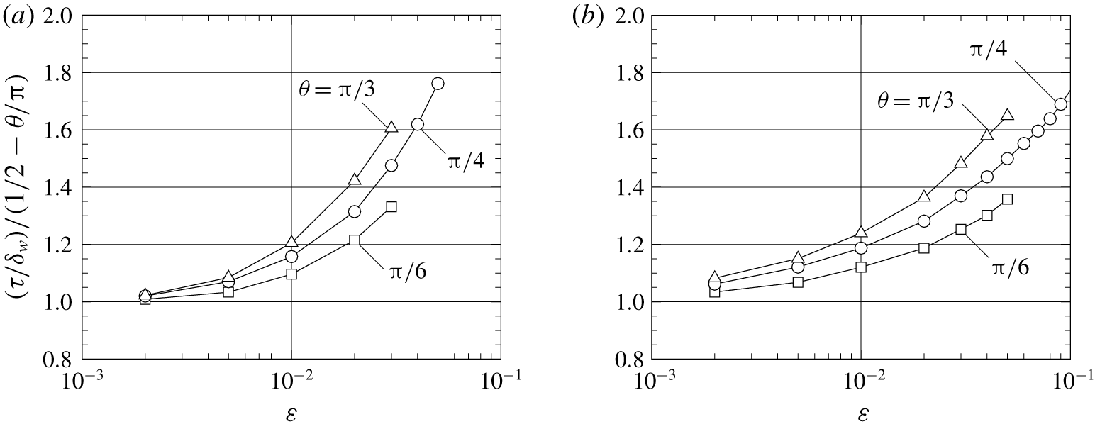
Figure 6. The normalized temperature
 $(\unicode[STIX]{x1D70F}/\unicode[STIX]{x1D6FF}_{w})/(1/2-\unicode[STIX]{x1D703}/\unicode[STIX]{x03C0})$
at the point
$(\unicode[STIX]{x1D70F}/\unicode[STIX]{x1D6FF}_{w})/(1/2-\unicode[STIX]{x1D703}/\unicode[STIX]{x03C0})$
at the point
 $(x_{1},x_{2})=(a\unicode[STIX]{x1D700}^{\unicode[STIX]{x1D6FC}}\cos \unicode[STIX]{x1D703},-1/2+a\unicode[STIX]{x1D700}^{\unicode[STIX]{x1D6FC}}\sin \unicode[STIX]{x1D703})$
for various
$(x_{1},x_{2})=(a\unicode[STIX]{x1D700}^{\unicode[STIX]{x1D6FC}}\cos \unicode[STIX]{x1D703},-1/2+a\unicode[STIX]{x1D700}^{\unicode[STIX]{x1D6FC}}\sin \unicode[STIX]{x1D703})$
for various
 $\unicode[STIX]{x1D700}$
. (a)
$\unicode[STIX]{x1D700}$
. (a)
 $(\unicode[STIX]{x1D6FC},a)=(1/2,3)$
, (b)
$(\unicode[STIX]{x1D6FC},a)=(1/2,3)$
, (b)
 $(\unicode[STIX]{x1D6FC},a)=(1/3,3/2)$
. The symbols represent the numerical results, which are connected by the solid lines.
$(\unicode[STIX]{x1D6FC},a)=(1/3,3/2)$
. The symbols represent the numerical results, which are connected by the solid lines.

Figure 7. The normalized radial flow velocity
 $\unicode[STIX]{x1D6FF}_{w}^{-1}a|u_{r}|/\text{sin}\,2\unicode[STIX]{x1D703}$
at the point
$\unicode[STIX]{x1D6FF}_{w}^{-1}a|u_{r}|/\text{sin}\,2\unicode[STIX]{x1D703}$
at the point
 $(x_{1}(\unicode[STIX]{x1D700}),x_{2}(\unicode[STIX]{x1D700}))=(a\unicode[STIX]{x1D700}^{\unicode[STIX]{x1D6FC}}\cos \unicode[STIX]{x1D703},-1/2+a\unicode[STIX]{x1D700}^{\unicode[STIX]{x1D6FC}}\sin \unicode[STIX]{x1D703})$
for various
$(x_{1}(\unicode[STIX]{x1D700}),x_{2}(\unicode[STIX]{x1D700}))=(a\unicode[STIX]{x1D700}^{\unicode[STIX]{x1D6FC}}\cos \unicode[STIX]{x1D703},-1/2+a\unicode[STIX]{x1D700}^{\unicode[STIX]{x1D6FC}}\sin \unicode[STIX]{x1D703})$
for various
 $\unicode[STIX]{x1D700}$
. (a)
$\unicode[STIX]{x1D700}$
. (a)
 $(\unicode[STIX]{x1D6FC},a)=(1/2,1)$
, (b)
$(\unicode[STIX]{x1D6FC},a)=(1/2,1)$
, (b)
 $(\unicode[STIX]{x1D6FC},a)=(1/3,1/2)$
. See the caption of figure 6.
$(\unicode[STIX]{x1D6FC},a)=(1/3,1/2)$
. See the caption of figure 6.
Finally, we consider the radial component of the flow velocity
 $u_{r}$
. In figure 7, we plot
$u_{r}$
. In figure 7, we plot
 $\unicode[STIX]{x1D6FF}_{w}^{-1}a|u_{r}|/\sin 2\unicode[STIX]{x1D703}$
at
$\unicode[STIX]{x1D6FF}_{w}^{-1}a|u_{r}|/\sin 2\unicode[STIX]{x1D703}$
at
 $(x_{1},x_{2})=(a\unicode[STIX]{x1D700}^{\unicode[STIX]{x1D6FC}}\cos \unicode[STIX]{x1D703},-1/2+a\unicode[STIX]{x1D700}^{\unicode[STIX]{x1D6FC}}\sin \unicode[STIX]{x1D703})$
for various
$(x_{1},x_{2})=(a\unicode[STIX]{x1D700}^{\unicode[STIX]{x1D6FC}}\cos \unicode[STIX]{x1D703},-1/2+a\unicode[STIX]{x1D700}^{\unicode[STIX]{x1D6FC}}\sin \unicode[STIX]{x1D703})$
for various
 $\unicode[STIX]{x1D700}$
in the cases of
$\unicode[STIX]{x1D700}$
in the cases of
 $(\unicode[STIX]{x1D6FC},a)=(1/2,1)$
in panel (a) and
$(\unicode[STIX]{x1D6FC},a)=(1/2,1)$
in panel (a) and
 $(\unicode[STIX]{x1D6FC},a)=(1/3,1/2)$
in panel (b). Again each panel contains the results for three different values of
$(\unicode[STIX]{x1D6FC},a)=(1/3,1/2)$
in panel (b). Again each panel contains the results for three different values of
 $\unicode[STIX]{x1D703}$
 $(\unicode[STIX]{x1D703}=\unicode[STIX]{x03C0}/6,\unicode[STIX]{x03C0}/4,\unicode[STIX]{x03C0}/3)$
. If the asymptotic behaviour shown in (4.5) holds, the double-log plot of
$(\unicode[STIX]{x1D703}=\unicode[STIX]{x03C0}/6,\unicode[STIX]{x03C0}/4,\unicode[STIX]{x03C0}/3)$
. If the asymptotic behaviour shown in (4.5) holds, the double-log plot of
 $\unicode[STIX]{x1D6FF}_{w}^{-1}a|u_{r}|/\sin 2\unicode[STIX]{x1D703}$
as a function of
$\unicode[STIX]{x1D6FF}_{w}^{-1}a|u_{r}|/\sin 2\unicode[STIX]{x1D703}$
as a function of
 $\unicode[STIX]{x1D700}$
for a given
$\unicode[STIX]{x1D700}$
for a given
 $(\unicode[STIX]{x1D6FC},a,\unicode[STIX]{x1D703})$
should approach a line with the slope
$(\unicode[STIX]{x1D6FC},a,\unicode[STIX]{x1D703})$
should approach a line with the slope
 $1-\unicode[STIX]{x1D6FC}$
as
$1-\unicode[STIX]{x1D6FC}$
as
 $\unicode[STIX]{x1D700}{\searrow}0$
. In figure 7, we actually observe that each plot tends to approach a line with the slope
$\unicode[STIX]{x1D700}{\searrow}0$
. In figure 7, we actually observe that each plot tends to approach a line with the slope
 $1/2$
in panel (a) and a line with the slope
$1/2$
in panel (a) and a line with the slope
 $2/3$
in panel (b), independently of
$2/3$
in panel (b), independently of
 $\unicode[STIX]{x1D703}$
, as
$\unicode[STIX]{x1D703}$
, as
 $\unicode[STIX]{x1D700}$
is reduced. This supports again the asymptotic behaviour of
$\unicode[STIX]{x1D700}$
is reduced. This supports again the asymptotic behaviour of
 $u_{r}$
shown in (4.5).
$u_{r}$
shown in (4.5).
To summarize, the numerical results given above support the presence of the cross-over region between the Knudsen zone and the outer region in which the macroscopic variables behave in the same manner as
 $\unicode[STIX]{x1D70F}/\unicode[STIX]{x1D6FF}_{w}\sim (1/2-\unicode[STIX]{x1D703}/\unicode[STIX]{x03C0})$
and
$\unicode[STIX]{x1D70F}/\unicode[STIX]{x1D6FF}_{w}\sim (1/2-\unicode[STIX]{x1D703}/\unicode[STIX]{x03C0})$
and
 $u_{r}/\unicode[STIX]{x1D6FF}_{w}\sim (\unicode[STIX]{x1D700}/r)\sin 2\unicode[STIX]{x1D703}$
.
$u_{r}/\unicode[STIX]{x1D6FF}_{w}\sim (\unicode[STIX]{x1D700}/r)\sin 2\unicode[STIX]{x1D703}$
.
5 Concluding remarks
In this paper, we considered a slightly rarefied gas confined between two parallel plates with a discontinuous surface temperature distribution and investigated its steady behaviour. We aimed at extending the conventional GSF theory, which assumes smooth boundary data, to the case in which the boundary temperature has a jump discontinuity, in the simplest case where the boundary is a flat surface. With the aid of rich accumulation of the results known for the case of smooth boundary data, we carried out an asymptotic analysis of the Boltzmann system for small Knudsen numbers based on the matched asymptotic expansion, which employs Sone’s asymptotics as the outer solution and a newly introduced kinetic boundary layer (the Knudsen zone) as the inner solution. The analysis was carried out to the first order of the Knudsen number and, in particular, an appropriate form of the ‘slip boundary condition’ for the flow driven by a discontinuous surface temperature was identified. The main results obtained in this paper are summarized as follows:
-
(1) The conventional slip-flow theory, which assumes the smoothness of the boundary data, breaks down near the point where the surface temperature is discontinuous. In this local region (or the Knudsen zone), the solution varies in the scale of the mean free path in both normal and tangential directions to the boundary.
-
(2) The half-space boundary-value problem associated with the Knudsen zone for a discontinuous surface temperature over a flat boundary was formulated. The asymptotic form of the solution at far field was derived.
-
(3) In the Knudsen zone, the flow velocity decreases with distance in proportion to the reciprocal of the distance. In the far field of the Knudsen zone, the flow velocity has radially diverging or converging streamlines depending on the hotter or colder side.
-
(4) The overall flow velocity in the channel is expressed as
$u_{i}=\unicode[STIX]{x1D700}u_{iH1}+O(\unicode[STIX]{x1D700}^{2})$
and the essential term
$u_{iH1}$
is described by the Stokes equation for an incompressible fluid with the no-slip boundary condition. It also satisfies a singular source/sink condition located at the point of discontinuity, which diverges in approaching the point of discontinuity. The analysis of the half-space problem (i.e. the Knudsen-zone problem) mentioned above determines the multiplicative factor (
$\unicode[STIX]{x1D6E4}_{Z}^{(1)}$
) of this singular source/sink condition. -
(5) The result of the direct numerical analysis based on the BGK model for a rarefied gas flow in a square vessel with a discontinuous surface temperature is consistent with that of the asymptotic analysis.


In this way, the ‘slip boundary condition’ for the flow induced by a discontinuous surface temperature is qualitatively different from those for the thermal-creep or thermal-stress slip flow.
Acknowledgements
This work was supported by JSPS KAKENHI grant no. 17K06146. The authors thank Mr K. Oniyama for his assistance in the numerical analysis carried out in § 4. A part of numerical computations was carried out using the supercomputer of ACCMS, Kyoto University.
Declaration of interests
The authors report no conflict of interest.
Appendix A. Derivation of (3.34) and (3.35)
In this appendix, we outline the derivation of (3.34) and (3.35). We focus on the derivation of the Hilbert part, since the derivation of the Knudsen-layer part is parallel to the derivation of boundary conditions for the Stokes system. Throughout this appendix, the subscript
 $Z0$
will be omitted.
$Z0$
will be omitted.
Let us assume that, for some small constant
 $0<\unicode[STIX]{x1D6FF}\ll 1$
, the length scale of variation is
$0<\unicode[STIX]{x1D6FF}\ll 1$
, the length scale of variation is
 $\unicode[STIX]{x1D6FF}^{-1}$
in the region
$\unicode[STIX]{x1D6FF}^{-1}$
in the region
 $(\,y_{1}^{2}+y_{2}^{2})^{1/2}>\unicode[STIX]{x1D6FF}^{-1}$
, i.e.
$(\,y_{1}^{2}+y_{2}^{2})^{1/2}>\unicode[STIX]{x1D6FF}^{-1}$
, i.e.
 $\unicode[STIX]{x2202}\unicode[STIX]{x1D719}/\unicode[STIX]{x2202}y_{i}=O(\unicode[STIX]{x1D6FF}\,\unicode[STIX]{x1D719})$
. The validity of this assumption is verified if such a solution is obtained. Then, introducing new variables
$\unicode[STIX]{x2202}\unicode[STIX]{x1D719}/\unicode[STIX]{x2202}y_{i}=O(\unicode[STIX]{x1D6FF}\,\unicode[STIX]{x1D719})$
. The validity of this assumption is verified if such a solution is obtained. Then, introducing new variables
 $$\begin{eqnarray}x_{i}=\unicode[STIX]{x1D6FF}\,y_{i},\end{eqnarray}$$
the velocity distribution function is sought in the form
 $\unicode[STIX]{x1D719}=\unicode[STIX]{x1D719}(x_{1},x_{2},\unicode[STIX]{x1D709}_{i})$
. Then,
$\unicode[STIX]{x1D719}=\unicode[STIX]{x1D719}(x_{1},x_{2},\unicode[STIX]{x1D709}_{i})$
. Then,
 $\unicode[STIX]{x1D719}$
satisfies the linearized Boltzmann equation of the form
$\unicode[STIX]{x1D719}$
satisfies the linearized Boltzmann equation of the form
 $$\begin{eqnarray}\unicode[STIX]{x1D709}_{1}\unicode[STIX]{x2202}_{1}\unicode[STIX]{x1D719}+\unicode[STIX]{x1D709}_{2}\unicode[STIX]{x2202}_{2}\unicode[STIX]{x1D719}=\frac{1}{\unicode[STIX]{x1D6FF}}{\mathcal{L}}(\unicode[STIX]{x1D719}).\end{eqnarray}$$
Thus,
 $\unicode[STIX]{x1D6FF}$
plays the role of a small Knudsen number and one can seek an asymptotic solution for small values of
$\unicode[STIX]{x1D6FF}$
plays the role of a small Knudsen number and one can seek an asymptotic solution for small values of
 $\unicode[STIX]{x1D6FF}$
in the form
$\unicode[STIX]{x1D6FF}$
in the form
 $$\begin{eqnarray}\displaystyle & \displaystyle \unicode[STIX]{x1D719}=\unicode[STIX]{x1D719}_{H}+\unicode[STIX]{x1D719}_{K}, & \displaystyle\end{eqnarray}$$
 $$\begin{eqnarray}\displaystyle & \displaystyle \unicode[STIX]{x1D719}_{H}=\unicode[STIX]{x1D719}_{H0}+\unicode[STIX]{x1D719}_{H1}\unicode[STIX]{x1D6FF}+\cdots \,, & \displaystyle\end{eqnarray}$$
 $$\begin{eqnarray}\displaystyle & \displaystyle \unicode[STIX]{x1D719}_{K}=\unicode[STIX]{x1D719}_{K1}\unicode[STIX]{x1D6FF}+\cdots \,, & \displaystyle\end{eqnarray}$$
 $\unicode[STIX]{x1D719}_{H}$
is the Hilbert solution and
$\unicode[STIX]{x1D719}_{H}$
is the Hilbert solution and
 $\unicode[STIX]{x1D719}_{K}$
is the Knudsen-layer correction near the boundary
$\unicode[STIX]{x1D719}_{K}$
is the Knudsen-layer correction near the boundary
 $x_{1}=0$
. The corresponding macroscopic quantities
$x_{1}=0$
. The corresponding macroscopic quantities
 $\unicode[STIX]{x1D714}$
,
$\unicode[STIX]{x1D714}$
,
 $u_{i}$
,
$u_{i}$
,
 $\unicode[STIX]{x1D70F}$
and
$\unicode[STIX]{x1D70F}$
and
 $P$
are expressed similarly as
$P$
are expressed similarly as  $$\begin{eqnarray}\displaystyle & \displaystyle h=h_{H}+h_{K}, & \displaystyle\end{eqnarray}$$
 $$\begin{eqnarray}\displaystyle & \displaystyle h_{H}=h_{H0}+h_{H1}\unicode[STIX]{x1D6FF}+\cdots \,, & \displaystyle\end{eqnarray}$$
 $$\begin{eqnarray}\displaystyle & \displaystyle h_{K}=h_{K1}\unicode[STIX]{x1D6FF}+\cdots \,, & \displaystyle\end{eqnarray}$$
 $h=\unicode[STIX]{x1D714}$
,
$h=\unicode[STIX]{x1D714}$
,
 $u_{i}$
,
$u_{i}$
,
 $\unicode[STIX]{x1D70F}$
and
$\unicode[STIX]{x1D70F}$
and
 $P$
. Then, the analysis is analogous to § 2 (
$P$
. Then, the analysis is analogous to § 2 (
 $\unicode[STIX]{x1D6FF}$
corresponds to
$\unicode[STIX]{x1D6FF}$
corresponds to
 $\unicode[STIX]{x1D700}$
). In particular, the boundary conditions for the flow velocity and temperature on the lower half of the boundary,
$\unicode[STIX]{x1D700}$
). In particular, the boundary conditions for the flow velocity and temperature on the lower half of the boundary,
 $x_{1}=0$
and
$x_{1}=0$
and
 $x_{2}<0$
, are obtained from those on the upper half by replacing
$x_{2}<0$
, are obtained from those on the upper half by replacing
 $\unicode[STIX]{x1D70F}_{w}$
by
$\unicode[STIX]{x1D70F}_{w}$
by
 $-\unicode[STIX]{x1D70F}_{w}$
. We shall obtain the asymptotic solution satisfying the required symmetry (3.32).
$-\unicode[STIX]{x1D70F}_{w}$
. We shall obtain the asymptotic solution satisfying the required symmetry (3.32).
Order
$\unicode[STIX]{x1D6FF}^{0}$

We solve (2.11)–(2.12) for
 $m=0$
with
$m=0$
with
 $\unicode[STIX]{x2202}_{3}=0$
and
$\unicode[STIX]{x2202}_{3}=0$
and
 $u_{3H0}=0$
under the boundary conditions
$u_{3H0}=0$
under the boundary conditions
 $$\begin{eqnarray}\displaystyle & \displaystyle u_{iH0}=0,\quad \unicode[STIX]{x1D70F}_{H0}=\pm \unicode[STIX]{x1D70F}_{w},\quad (x_{1}=0,\pm x_{2}>0), & \displaystyle\end{eqnarray}$$
 $$\begin{eqnarray}\displaystyle & \displaystyle u_{iH0}\rightarrow 0,\quad \unicode[STIX]{x1D70F}_{H0}\rightarrow \frac{2\unicode[STIX]{x1D70F}_{w}}{\unicode[STIX]{x03C0}}\unicode[STIX]{x1D703},\quad P_{H0}\rightarrow 0,\quad (r\rightarrow \infty ), & \displaystyle\end{eqnarray}$$
 $r=\sqrt{x_{1}^{2}+x_{2}^{2}}$
and
$r=\sqrt{x_{1}^{2}+x_{2}^{2}}$
and
 $\unicode[STIX]{x1D703}=\text{Arctan}(x_{2}/x_{1})$
. The solution is given by
$\unicode[STIX]{x1D703}=\text{Arctan}(x_{2}/x_{1})$
. The solution is given by  $$\begin{eqnarray}P_{H0}=0,\quad u_{iH0}=0,\quad P_{H1}=0,\quad \unicode[STIX]{x1D70F}_{H0}=\frac{2\unicode[STIX]{x1D70F}_{w}}{\unicode[STIX]{x03C0}}\unicode[STIX]{x1D703},\end{eqnarray}$$
where
 $P_{H1}$
is determined up to an additive constant. Thus, the velocity distribution function is obtained as
$P_{H1}$
is determined up to an additive constant. Thus, the velocity distribution function is obtained as
 $$\begin{eqnarray}\unicode[STIX]{x1D719}_{H0}=\frac{2\unicode[STIX]{x1D70F}_{w}}{\unicode[STIX]{x03C0}}\left(\unicode[STIX]{x1D709}_{j}^{2}-\frac{5}{2}\right)\unicode[STIX]{x1D703}.\end{eqnarray}$$
There is no Knudsen-layer correction required at this order.
Order
$\unicode[STIX]{x1D6FF}^{1}$

We solve (2.12) for
 $m=1$
with
$m=1$
with
 $\unicode[STIX]{x2202}_{3}=0$
and
$\unicode[STIX]{x2202}_{3}=0$
and
 $u_{3H1}=0$
under the boundary conditions
$u_{3H1}=0$
under the boundary conditions
 $$\begin{eqnarray}\displaystyle & \displaystyle u_{rH1}=u_{\unicode[STIX]{x1D703}H1}=0,\quad \unicode[STIX]{x1D70F}_{H1}=\mp \frac{2\unicode[STIX]{x1D70F}_{w}c_{1}^{(0)}}{\unicode[STIX]{x03C0}}\frac{1}{r},\quad \left(\unicode[STIX]{x1D703}=\pm \frac{\unicode[STIX]{x03C0}}{2},\,r>0\right), & \displaystyle\end{eqnarray}$$
 $$\begin{eqnarray}\displaystyle & \displaystyle u_{iH1}\rightarrow 0,\quad \unicode[STIX]{x1D70F}_{H1}\rightarrow 0,\quad P_{H1}\rightarrow 0,\quad (r\rightarrow \infty ), & \displaystyle\end{eqnarray}$$
 $u_{rHm}$
and
$u_{rHm}$
and
 $u_{\unicode[STIX]{x1D703}Hm}$
are the radial and circumferential components of
$u_{\unicode[STIX]{x1D703}Hm}$
are the radial and circumferential components of
 $u_{iHm}$
in the polar coordinate system centred at the origin. From the last condition of (A 8b
), the additive constant in
$u_{iHm}$
in the polar coordinate system centred at the origin. From the last condition of (A 8b
), the additive constant in
 $P_{H1}$
must vanish. Solving the problem, we have
$P_{H1}$
must vanish. Solving the problem, we have  $$\begin{eqnarray}\displaystyle & \displaystyle P_{H1}=0,\quad u_{rH1}=\unicode[STIX]{x1D70F}_{w}\frac{\unicode[STIX]{x1D6E4}_{Z}^{(1)}\sin 2\unicode[STIX]{x1D703}}{r},\quad u_{\unicode[STIX]{x1D703}H1}=0, & \displaystyle\end{eqnarray}$$
 $$\begin{eqnarray}\displaystyle & \displaystyle P_{H2}=\unicode[STIX]{x1D70F}_{w}\frac{2\unicode[STIX]{x1D6FE}_{1}\unicode[STIX]{x1D6E4}_{Z}^{(1)}}{r^{2}}\sin 2\unicode[STIX]{x1D703},\quad \unicode[STIX]{x1D70F}_{H1}=-\frac{2}{\unicode[STIX]{x03C0}}\unicode[STIX]{x1D70F}_{w}c_{1}^{(0)}\frac{\sin \unicode[STIX]{x1D703}}{r}, & \displaystyle\end{eqnarray}$$
 $\unicode[STIX]{x1D6E4}_{Z}^{(1)}$
is an undetermined constant and
$\unicode[STIX]{x1D6E4}_{Z}^{(1)}$
is an undetermined constant and
 $P_{H2}$
is determined up to an additive constant. From (2.43), the velocity distribution function is given by
$P_{H2}$
is determined up to an additive constant. From (2.43), the velocity distribution function is given by  $$\begin{eqnarray}\displaystyle & \displaystyle \frac{\unicode[STIX]{x1D719}_{H1}}{\unicode[STIX]{x1D70F}_{w}}=2\unicode[STIX]{x1D709}_{r}\frac{\unicode[STIX]{x1D6E4}_{Z}^{(1)}\sin 2\unicode[STIX]{x1D703}}{r}-\left(\unicode[STIX]{x1D709}_{j}^{2}-\frac{5}{2}\right)\frac{2}{\unicode[STIX]{x03C0}}c_{1}^{(0)}\frac{\sin \unicode[STIX]{x1D703}}{r}-\frac{2}{\unicode[STIX]{x03C0}}A(\unicode[STIX]{x1D709})\frac{\unicode[STIX]{x1D709}_{\unicode[STIX]{x1D703}}}{r}, & \displaystyle\end{eqnarray}$$
 $$\begin{eqnarray}\displaystyle & \displaystyle \frac{\unicode[STIX]{x1D719}_{K1}}{\unicode[STIX]{x1D70F}_{w}}=-\frac{2}{\unicode[STIX]{x03C0}}\frac{1}{x_{2}}\unicode[STIX]{x1D711}_{1}^{(0)}(\,y_{1},\unicode[STIX]{x1D709}_{1},\unicode[STIX]{x1D709}), & \displaystyle\end{eqnarray}$$
 $\unicode[STIX]{x1D709}=(\unicode[STIX]{x1D709}_{j}^{2})^{1/2}$
and
$\unicode[STIX]{x1D709}=(\unicode[STIX]{x1D709}_{j}^{2})^{1/2}$
and
 $y_{1}=x_{1}/\unicode[STIX]{x1D6FF}$
. The Knudsen-layer corrections for the macroscopic quantities are summarized as
$y_{1}=x_{1}/\unicode[STIX]{x1D6FF}$
. The Knudsen-layer corrections for the macroscopic quantities are summarized as  $$\begin{eqnarray}\displaystyle & \displaystyle u_{rK1}=u_{\unicode[STIX]{x1D703}K1}=0,\quad \unicode[STIX]{x1D714}_{K1}=-\frac{2}{\unicode[STIX]{x03C0}}\frac{1}{x_{2}}\unicode[STIX]{x1D6FA}_{1}^{(0)}(\,y_{1}), & \displaystyle\end{eqnarray}$$
 $$\begin{eqnarray}\displaystyle & \displaystyle \unicode[STIX]{x1D70F}_{K1}=-\frac{2}{\unicode[STIX]{x03C0}}\frac{1}{x_{2}}\unicode[STIX]{x1D6E9}_{1}^{(0)}(\,y_{1}),\quad P_{K1}=-\frac{2}{\unicode[STIX]{x03C0}}\frac{1}{x_{2}}(\unicode[STIX]{x1D6FA}_{1}^{(0)}(\,y_{1})+\unicode[STIX]{x1D6E9}_{1}^{(0)}(\,y_{1})). & \displaystyle\end{eqnarray}$$
Order
$\unicode[STIX]{x1D6FF}^{2}$

For the purpose of the present study, we do not need the information of the far-field asymptotics to the order
 $\unicode[STIX]{x1D6FF}^{2}$
. However, it is important for the numerical analysis as well as for a theoretical insight. Therefore, we present the result.
$\unicode[STIX]{x1D6FF}^{2}$
. However, it is important for the numerical analysis as well as for a theoretical insight. Therefore, we present the result.
If we continue the analysis in § 2 to the order of
 $\unicode[STIX]{x1D700}^{2}$
or referring to chap. 3 of Sone (Reference Sone2007) (or to Takata & Hattori (Reference Takata and Hattori2012)), the boundary conditions on
$\unicode[STIX]{x1D700}^{2}$
or referring to chap. 3 of Sone (Reference Sone2007) (or to Takata & Hattori (Reference Takata and Hattori2012)), the boundary conditions on
 $x_{1}=0$
are given by
$x_{1}=0$
are given by
 $$\begin{eqnarray}\displaystyle & \displaystyle u_{rH2}=\pm 2\unicode[STIX]{x1D70F}_{w}\frac{\unicode[STIX]{x1D6E4}_{Z}^{(1)}b_{1}^{(1)}+{\displaystyle \frac{c_{1}^{(0)}b_{2}^{(1)}+b_{3}^{(1)}}{\unicode[STIX]{x03C0}}}}{r^{2}},\quad u_{\unicode[STIX]{x1D703}H2}=0,\quad \unicode[STIX]{x1D70F}_{H2}=0,\quad \left(\unicode[STIX]{x1D703}=\pm \frac{\unicode[STIX]{x03C0}}{2},r>0\right), & \displaystyle \nonumber\\ \displaystyle & & \displaystyle\end{eqnarray}$$
 $$\begin{eqnarray}\displaystyle & \displaystyle u_{iH2}\rightarrow 0,\quad \unicode[STIX]{x1D70F}_{H2}\rightarrow 0,\quad P_{H2}\rightarrow 0,\quad (r\rightarrow \infty ). & \displaystyle\end{eqnarray}$$
 $P_{H2}$
to be zero. Finding solutions to (2.12) for
$P_{H2}$
to be zero. Finding solutions to (2.12) for
 $m=2$
with
$m=2$
with
 $\unicode[STIX]{x2202}_{3}=0$
and
$\unicode[STIX]{x2202}_{3}=0$
and
 $u_{3H2}=0$
under these conditions, we have
$u_{3H2}=0$
under these conditions, we have  $$\begin{eqnarray}\displaystyle & \displaystyle \frac{u_{rH2}}{\unicode[STIX]{x1D70F}_{w}}=\frac{-3\unicode[STIX]{x1D6E4}_{Z}^{(2)}(\sin 3\unicode[STIX]{x1D703}+\sin \unicode[STIX]{x1D703})+2\left(\unicode[STIX]{x1D6E4}_{Z}^{(1)}b_{1}^{(1)}+{\displaystyle \frac{c_{1}^{(0)}b_{2}^{(1)}+b_{3}^{(1)}}{\unicode[STIX]{x03C0}}}\right)\sin \unicode[STIX]{x1D703}}{r^{2}}, & \displaystyle\end{eqnarray}$$
 $$\begin{eqnarray}\displaystyle & \displaystyle \frac{u_{\unicode[STIX]{x1D703}H2}}{\unicode[STIX]{x1D70F}_{w}}=\frac{\unicode[STIX]{x1D6E4}_{Z}^{(2)}(\cos 3\unicode[STIX]{x1D703}+3\cos \unicode[STIX]{x1D703})-2\left(\unicode[STIX]{x1D6E4}_{Z}^{(1)}b_{1}^{(1)}+{\displaystyle \frac{c_{1}^{(0)}b_{2}^{(1)}+b_{3}^{(1)}}{\unicode[STIX]{x03C0}}}\right)\cos \unicode[STIX]{x1D703}}{r^{2}}, & \displaystyle\end{eqnarray}$$
 $$\begin{eqnarray}\displaystyle & \displaystyle \frac{\unicode[STIX]{x1D70F}_{H2}}{\unicode[STIX]{x1D70F}_{w}}=\frac{\unicode[STIX]{x1D6EC}_{Z}^{(2)}}{r^{2}}\sin 2\unicode[STIX]{x1D703}, & \displaystyle\end{eqnarray}$$
 $\unicode[STIX]{x1D6E4}_{Z}^{(2)}$
and
$\unicode[STIX]{x1D6E4}_{Z}^{(2)}$
and
 $\unicode[STIX]{x1D6EC}_{Z}^{(2)}$
are undetermined constants. It is worth noting that the flow velocity is a special case of plane flows around a corner (Moffatt Reference Moffatt1964). The velocity distribution function is then given by
$\unicode[STIX]{x1D6EC}_{Z}^{(2)}$
are undetermined constants. It is worth noting that the flow velocity is a special case of plane flows around a corner (Moffatt Reference Moffatt1964). The velocity distribution function is then given by  $$\begin{eqnarray}\displaystyle \frac{\unicode[STIX]{x1D719}_{H2}}{\unicode[STIX]{x1D70F}_{w}} & = & \displaystyle \frac{2\unicode[STIX]{x1D6FE}_{1}\unicode[STIX]{x1D6E4}_{Z}^{(1)}}{r^{2}}\sin 2\unicode[STIX]{x1D703}+\left(\unicode[STIX]{x1D709}_{j}^{2}-\frac{5}{2}\right)\frac{\unicode[STIX]{x1D6EC}_{Z}^{(2)}}{r^{2}}\sin 2\unicode[STIX]{x1D703}\nonumber\\ \displaystyle & & \displaystyle -\,2\unicode[STIX]{x1D6E4}_{Z}^{(2)}\frac{3\unicode[STIX]{x1D709}_{r}(\sin 3\unicode[STIX]{x1D703}+\sin \unicode[STIX]{x1D703})-\unicode[STIX]{x1D709}_{\unicode[STIX]{x1D703}}(\cos 3\unicode[STIX]{x1D703}+3\cos \unicode[STIX]{x1D703})}{r^{2}}\nonumber\\ \displaystyle & & \displaystyle +\,4\left(\unicode[STIX]{x1D6E4}_{Z}^{(1)}b_{1}^{(1)}+\frac{c_{1}^{(0)}b_{2}^{(1)}+b_{3}^{(1)}}{\unicode[STIX]{x03C0}}\right)\frac{\unicode[STIX]{x1D709}_{r}\sin \unicode[STIX]{x1D703}-\unicode[STIX]{x1D709}_{\unicode[STIX]{x1D703}}\cos \unicode[STIX]{x1D703}}{r^{2}}\nonumber\\ \displaystyle & & \displaystyle -\,\frac{2}{\unicode[STIX]{x03C0}}c_{1}^{(0)}\left(\frac{\unicode[STIX]{x1D709}_{r}\sin \unicode[STIX]{x1D703}-\unicode[STIX]{x1D709}_{\unicode[STIX]{x1D703}}\cos \unicode[STIX]{x1D703}}{r^{2}}\right)A(\unicode[STIX]{x1D709})\nonumber\\ \displaystyle & & \displaystyle +\,\unicode[STIX]{x1D6E4}_{Z}^{(1)}\left(\frac{(\unicode[STIX]{x1D709}_{r}^{2}-\unicode[STIX]{x1D709}_{\unicode[STIX]{x1D703}}^{2})\sin 2\unicode[STIX]{x1D703}-2\unicode[STIX]{x1D709}_{r}\unicode[STIX]{x1D709}_{\unicode[STIX]{x1D703}}\cos 2\unicode[STIX]{x1D703}}{r^{2}}\right)B(\unicode[STIX]{x1D709})+\frac{4}{\unicode[STIX]{x03C0}}\frac{\unicode[STIX]{x1D709}_{r}\unicode[STIX]{x1D709}_{\unicode[STIX]{x1D703}}}{r^{2}}F(\unicode[STIX]{x1D709}),\end{eqnarray}$$
 $$\begin{eqnarray}\frac{\unicode[STIX]{x1D719}_{K2}}{\unicode[STIX]{x1D70F}_{w}}=\frac{\unicode[STIX]{x1D709}_{2}}{x_{2}^{2}}\left(2\unicode[STIX]{x1D6E4}_{Z}^{(1)}\unicode[STIX]{x1D711}_{1}^{(1)}(\,y_{1},\unicode[STIX]{x1D709}_{1},\unicode[STIX]{x1D709})+\frac{2}{\unicode[STIX]{x03C0}}c_{1}^{(0)}\unicode[STIX]{x1D711}_{2}^{(1)}(\,y_{1},\unicode[STIX]{x1D709}_{1},\unicode[STIX]{x1D709})+\frac{2}{\unicode[STIX]{x03C0}}\unicode[STIX]{x1D711}_{3}^{(1)}(\,y_{1},\unicode[STIX]{x1D709}_{1},\unicode[STIX]{x1D709})\right).\end{eqnarray}$$
 $$\begin{eqnarray}\displaystyle & \displaystyle \frac{u_{rK2}}{\unicode[STIX]{x1D70F}_{w}}=\frac{2}{x_{2}^{2}}\left(\unicode[STIX]{x1D6E4}_{Z}^{(1)}Y_{1}^{(1)}(\,y_{1})+\frac{c_{1}^{(0)}Y_{2}^{(1)}(\,y_{1})+Y_{3}^{(1)}(\,y_{1})}{\unicode[STIX]{x03C0}}\right)\sin \unicode[STIX]{x1D703}, & \displaystyle\end{eqnarray}$$
 $$\begin{eqnarray}\displaystyle & \displaystyle \frac{u_{\unicode[STIX]{x1D703}K2}}{\unicode[STIX]{x1D70F}_{w}}=\frac{2}{x_{2}^{2}}\left(\unicode[STIX]{x1D6E4}_{Z}^{(1)}Y_{1}^{(1)}(\,y_{1})+\frac{c_{1}^{(0)}Y_{2}^{(1)}(\,y_{1})+Y_{3}^{(1)}(\,y_{1})}{\unicode[STIX]{x03C0}}\right)\cos \unicode[STIX]{x1D703}, & \displaystyle\end{eqnarray}$$
 $$\begin{eqnarray}\displaystyle & \displaystyle \unicode[STIX]{x1D714}_{K2}=\unicode[STIX]{x1D70F}_{K2}=P_{K2}=0. & \displaystyle\end{eqnarray}$$
Assembling the above results according to (A 3)–(A 4) and taking account the relations
 $\unicode[STIX]{x1D6FF}/x_{2}=1/y_{2}$
and
$\unicode[STIX]{x1D6FF}/x_{2}=1/y_{2}$
and
 $\unicode[STIX]{x1D6FF}/r=1/\widetilde{r}$
, we obtain (3.34) and (3.35).
$\unicode[STIX]{x1D6FF}/r=1/\widetilde{r}$
, we obtain (3.34) and (3.35).


 Open access