Abstract
Condition monitoring is used as a tool for maintenance management and function as input to decision support. Thus the key parameters in preventing severe damage to railway assets can be determined by automatic real-time monitoring. The technique of radio-frequency identification (RFID) is increasingly applied for the automatic real-time monitoring and control of railway assets, which employs radio waves without the use of physical contact. In this work, a 243-km2 area of Kuala Lumpur was selected. Because of its large size, determining the locations in which to install the RFID readers for monitoring the bogie components in the Kuala Lumpur railway system is a very complex task. The task involved three challenges: first, finding an optimal evolutionary method for railway network planning in order to deploy the RFID system in a large-area; second, identifying the large area that involved functional features; third, determining which station or stations should be given priority in applying the RFID system to achieve the most effective monitoring of the trains. The first challenge was solved by using a gradient-base cuckoo search algorithm for RFID system deployment. The second challenge was solved by determining all necessary information using geographic information system (GIS) resources. Because of the huge volume of data collected from GIS, it was found that the best method for eliminating data was to develop a new clustering model to separate the useful from the unuseful data and to identify the most suitable stations. Finally, the data set was reduced by developing a specific filter, and the information collected was tested by an analytic hierarchy process as a technique to determine the best stations for system monitoring and control. The results showed the success of the proposed method in solving the significant challenge of large-scale area conditions correlated with multi-objective RFID functions. The method provides high reliability in working with complex and dynamic data.
1 Introduction
Railway transportation plays a major role in a country’s economic growth. Rail is six times as energy-efficient as road travel and four times as economical. It is also safe and convenient [1]. Malaysian railways are currently facing a challenge in improving their reliability and speed in order to offer competitive services to the public and to enhance their importance as an alternative to road travel [2]. The scheduling of activities is crucial for achieving a well-functioning railway transportation system [3]. Maintenance activity is designed to prevent the unexpected breakdown of equipment, which may lead to reduced service quality and unexpected costs [4]. Rail transport in Malaysia involves heavy rail (including high-speed rail), monorail, and light rail transit (LRT) [5]. Table 1 presents the train lines in the Kuala Lumpur railway network. The main issues in railway maintenance are the lack of efficient and inexpensive technology for detecting problems and a lack of proper maintenance procedures [6]. Therefore, an effective railway maintenance strategy is needed to reduce overall costs while preserving the highest maintenance level [7].
Efficient planning of operations and maintenance can maximize the reliability and productivity of existing rail networks. Condition monitoring (CM) is a tool for maintenance management and function as input to decision support [8]. Products designed for condition monitoring of train vehicles are generally focused on bogie components, as the parameters of these critical components change during operation, posing safety issues [9]. Monitoring of train bogies is typically carried out by wayside monitoring devices installed along the track, as it would not be economical to monitor the condition of every component on a vehicle [10, 11].
Various types of wayside detection systems are commonly used today, including hot axle bearing (or hot axle box) detector (HABD), track acoustic array detector (TAAD), wheel impact load detector (WILD), weigh-in-motion detector, wheel profile detector (WPD), automatic vehicle identification (AVI) units, track circuit, fiber-optic sensor, and axle counter [12, 13].
In HABD systems, optical sensors are placed on the tracks. These sensors use infrared beams to measure critical parameters and then send the measured values wirelessly to the depot. However, a major obstacle to the use of optical sensors is the need to maintain a line of sight to detect the part status [9, 13, 14].
Wireless communication-based technology has recently been used to add layers of safety and reliability to the running of rail systems [15]. This has led to the need for intelligent condition monitoring systems using radio-frequency identification (RFID) devices. The RFID is used for automatic monitoring through radio waves without the use the physical contact [16]. It is also one of the main components in the Internet of Things (IoT) paradigm [17].
In this work, RFID is used to automatically identify the temperature and vibration of the gears and motor in each bogie system. For this task, the RFID reader positions must be specified [18]. Thus a small number of readers and a huge number of tags need to be deployed according to the longitudinal locations of the bogies in the railway stations. This gives rise to important considerations: (1) the number of readers needed to cover all tags, and (2) where the readers should be placed. These questions are considered hard network planning (NP) problems.
Optimization techniques are very helpful in solving NP-hard problems [19]. Several RFID network planning algorithms have been developed to optimize NP function parameters. In this work, we propose a gradient-based cuckoo search (GBCS) algorithm for solving the RFID network planning problem.
A particular challenge in the operation and management of RFID systems in Kuala Lumpur is the large area of Kuala Lumpur (about 243 km2). This large area presents a huge number of possibilities for the GBCS algorithm, which lowers its performance and increases the iteration time. Thus, in order to achieve high-quality results, organization of the topological information regarding the train systems is necessary.
In this paper, a GBCS algorithm is combined with an analytic hierarchy process (AHP) to identify the main train stations. RFID readers are then installed to record information on the train gears, motor temperature, and vibrations for condition monitoring and predictive maintenance purposes.
2 System Methodology
The methodology used in this work addresses the difficulties involved in railway RFID network planning in Kuala Lumpur, characterized by its large area, represented by a large number of railway stations, and the effect of RFID multi-objective network planning. The scenarios are developed in three main stages. The goal of the first stage is to find an efficient algorithm that can provide a superior method for solving large-scale RFID network planning problems. Here, the GBCS is found to be the best algorithm. In the second stage, the specific station positions are determined, along with all necessary information using geographic information system (GIS) resources (because there is no data set available). In the third stage, because of the large amount of data collected from GIS, the best method for eliminating data is found by developing a new clustering model to separate the useful from the unuseful data and to determine the most suitable stations. Finally, the data set is reduced by developing a specific filter, and the information obtained is tested using AHP to determine the best stations for system monitoring and control. The flow chart of the system methodogy is shown in Fig. 1. The methodolgy process includes three stages: 1) the first stage is to use GIS Date Collection and specify primary effective stations using filter; 2) the second stage is to specify effective stations using AHP; 3) the third stage is to apply optimization technique to install RFID in effective station.

Flow chart of the system methodology
2.1 Applying the Geographic Information System (GIS)
GIS is an information storage system that can integrate different types of data. It has been used as a tool to analyze specific map information [20].
Many researchers have used GIS with RFID systems in urban transportation management planning [21, 22]. In this study, GIS was used to identify the station positions (Fig. 2), the train movement in each station, and all other necessary information including the train line elevation from ground level, train line obstacles such as different line tunnels that could affect reader signals, and the number of train lines at a station, including details such as line name and its number.

Map of Kuala Lumpur stations
As shown in Table 1, there are 209 stations with 10 different rail lines, and the most suitable stations must be identified for installation of the RFID readers. Because of the vast amount of data collected from GIS, it was found that the best method for eliminating data and identifying the most suitable stations was by developing a new clustering model to separate the useful from the unuseful data. That means the filter will ignore the stations that have less lines and present the stations that have two or more than two lines. In other words, there is no benefit to put more than one station to control the same line's train. Also, if we have a station used for three or more lines, the stations with a single pass of the same line's train will be deleted or ignored because monitoring these trains will be covered through the effective stations. The effective stations were selected based on the following monitoring objective functions:
-
1.
Number of lines detected in a station, and the calculation method is shown in Eq. (1);
-
2.
Effective stations selected and not effective stations eliminated. The filter algorithum is to sum up the number of each station’s passing lines and consists of the station vector, as shown in Eq. (2).
where St is the number of lines passing the individual station, Tri = 1 if the line i passing the station, otherwise Tri = 0, and Stf is the stations vector. The filter categorized stations by the number of lines’ trains that pass through the station. The filter will ignore the stations that have less than two lines and present the stations that have two or more than two lines. This resulted in three classes: class 1, stations with two lines’ train passes; class 2, stations with three lines’ train passes; class 3, stations with four lines’ train passes. All the stations ranked in these three classes are shown in Table 2.
Based on the filtering results, only six stations can be effectively used for installing RFID readers. The TBS and KL-Central were assigned a higher rank, as they are used by four different lines, while the other stations (i.e. Subang Jaya, Masjid Jamek, Maluri, and Chan Sow Lin) were assigned a lower rank because they are used less by trains. Based on the classification filter results in Table 2 above, some stations rank takes the same values, such as TBS with KL-central, Masjid Jamek with Subang and, Maluri with Chan sow. Therefore, they cause a fuzzy in detecting the optimal stations. To solve this problem, there must be a technique that presents the prior stations. The researcher found that AHP is one of the best techniques that can help to decide which stations have taken priority for this mission. Therefore the numerical results in Table 2 present as input representation to AHP technique in order to choose the priority stations for best monitoring and control. All the data collected will be used as input for choosing the stations that can be used as monitoring centers for all the Kuala Lumpur trains.
2.2 Developing the AHP Technique
The AHP methodology was used to evaluate and determine which train stations are the most suitable to be used as monitoring centers in the Kuala Lumpur railway system. Due to the large number of stations based on different trains, it is necessary to determine the appropriate station or stations in which to apply the RFID system to achieve the most effective monitoring system. The huge number of stations for the 10 lines’ trains operating in Kuala Lumpur required the use of a decision process to eliminate unnecessary stations and identify robust stations that could monitor trains effectively. The selection of optimal stations is a difficult decision process for managers and transportation planners. AHP is an efficient technique that can be easily understood and used by decision-makers to simplify the process [23, 24].
AHP modeling consists of three main steps: (1) outlining the problem and structuring the decision hierarchy, (2) creating the pairwise comparison matrix, and (3) calculating the weights of the criteria. Using this three-point model, an AHP framework was developed to facilitate the process [25], and the following steps were proposed:
-
Step 1 Define the goal: The goal is to evaluate and select the proper stations to use as monitoring centers in the Kuala Lumpur railway systems.
-
Step 2 Identify the criteria for station selection: The maximum number of trains detected in a station and the minimum number of similar trains identified in a station are applied as criteria for station selection.
-
Step 3 Determine the stations to be used as monitoring centers: Highly effective stations are used in this study, namely TBS, KL-Central, Subang Jaya, Masjid Jamek, Maluri, and Chan Sow Lin stations, which are selected using the classification filter described in the previous section, the result is shown in Table 2.
-
Step 4 Construct a hierarchy framework for the analysis: The criteria are structured into a hierarchy descending from the overall objective to the various stages. The top level of the hierarchy represents the defined objective, while the second level consists of two criteria for the station selection. Finally, the bottom level of the hierarchy represents the station alternatives. Two zones are selected for the AHP process, where each zone represents a group of stations that can be correlated by neighborhood relationships based on the distance between stations, as shown in Fig. 3.
Fig. 3 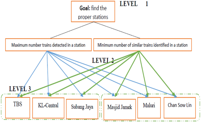
AHP process
-
Step 5 Collect empirical information and data after building the AHP hierarchy: This stage consists of measurement and collection of data, which involves creating a set of evaluators.
-
Step 6 Perform pairwise comparisons for each level of criteria: Pairwise comparison decision matrices are obtained from two evaluators having experience in the field of railway engineering. The authors, together with the evaluators, compare the importance of the selection criteria in pairwise fashion according to the goal of the decision problem. These decisions are then combined using the geometric mean at each hierarchy level to obtain the corresponding consensus. A relational scale of real numbers from 1 to 9 is used for ranking, as presented in Table 3.
Table 3 Scale of relative performance (pairwise comparison) [24]

The purpose of this scale is to determine to what degree one station is more important than another station with respect to the criteria. After completion of the pairwise comparison matrices, the weights of the criteria are calculated using the pseudo-code identification process shown in Fig. 4.

Priority station identification using the modified AHP technique
The results represent the priority station information used in the GBCS to determine optimal reader positions based on RFID objective functions.
2.3 Gradient-Based Cuckoo Search (GBCS)
This section presents the evolutionary algorithm used to solve the multi-objective functions based on correlations between actual tag positions and RFID reader propagation rate. A modified cuckoo search algorithm is correlated with the gradient of the objective function for this task [26, 27]. GBCS has proven to be a strong candidate algorithm for solving difficult optimization problems in large-scale areas. One of the most powerful features of GBCS search is the use of Lévy flight to generate a new solution. The Lévy flight technique focuses the search over a large area, as the steps are not restricted by area. Therefore, the use of the GBCS algorithm with small steps and occasional large jumps makes the GBCS unique among optimization algorithms, as it can be used efficiently in large-scale conditions with clustered big data [28, 29]. Thus, it can be a useful solution for RFID network planning in railway stations.
The main steps involved in this algorithm are as follows:
-
Step 1 Read and transfer AHP results to the computational board to read GIS images.
-
Step 2 Select proper stations for train monitoring.
-
Step 3 Automatically select station images and then use mouse clicks to generate tag coordinates.
-
Step 4 Evaluate the fitness value of each reader based on the objective functions used in the following equation:
The Friis transformation equation is used to determine the amount of power received from one antenna (with gain G1) when transmitted from another antenna (with gain G2), based on the distance (rmax) between them, and operating at wavelength λ or frequency f, as in Eq. (3) [30, 31]:
$$ P_{{\text{R}}} = P_{{\text{T}}} \times G_{\text{T}} \times G_{\text{R}} \times \left( {\frac{\lambda }{4 \times \pi }} \right)^{2} \times \frac{1}{{r_{ \text{max} }^{n} }} $$(3)where \( P_{{\text{R}}} \) is the power input tag, \( P_{{\text{T}}} \) is the power output reader, \( G_{\text{R}} \) is the reader antenna gain, \( G_{\text{T}} \) is the tag antenna gain, and λ is the wavelength. In free space, the path loss (PL) exponent n is set at 2, but in cluttered environments such as urban or suburban areas (with pipes and tunnels, etc.), the PL exponent n may vary from 1 to 4.
The propagation domain of the RFID reader (\( r_{ \text{max} } \)) can be determined from the set of the expressions (4), (5), and (6). Where Ldb is path loss in decibel, Lm is path loss in meter, C is light speed, C = 299792458 m/s, f is operating frequency, here f = 915.
The propagation range calculated in Eq. (6) is subject to the boundary conditions [31]
Where rtd, is the distance between the tag and reader in the working space, can be calculated by the following expression:
where \( x, y \) are the coordinates of the reader and \( x_{t} ,y_{t} \) are the coordinates of the tag.
The optimal number of RFID readers Ni is calculated using the formulae (8) and (9) [30]:
where covi is the coverage rate of tags in the propagation domains (RS). Ni is reader number in the working domain (TS). And k is the number of tags groups in the working domain.
The tag coverage rate cov in the specified area, which represents a significant and important objective function of RFID technology, is determined as expression 10: [30]
where cov is the coverage rate of the tags in the TS range, covi is the coverage rate of the tags specified within reader ith propagation range, Nt is the number of tags distributed in the working domain. The base of tags distribution Nt is dependent on: 1) the number of train pass through the station; 2) the number of car-sets of each train; 3) the number of bogie system in each car-set of train; 4) the number of electrical motor and gear in each bogie. Reader collisions usually occur in very dense environments where multiple readers try at the same time to interrogate tags. As a result of such situations, the unaccepted level of misreads can be reached. Reader collision avoidance objective can be defined as the expression (11).
where N is the number of readers. dis is the function to compute the distance between readers. (ri, rj) are the interference ranges for reader i and reader j, and (\( R_{i} ,R_{j} \)) is the position of the ith and jth reader in terms of the x−y axis respectively. The goal is to locate readers far from each other in order to avoid or minimize interference. According to the above formula the interference condition can be occurred when the sum of interrogation ranges of two readers (ri + rj) is greater than the center to center distance “d” between the same readers [(ri + rj) > d]. The interference rate can be calculated by the Eq. (12):
where covj is the coverage rate of the tags specified within reader jth propagation range.
The formulas presented above will be applied in the set of evaluation functions as an objective function [32]. In the original algorithm, when new nests are generated from the replaced nests via a random step, the magnitude and the direction of the step are both random.
Notation x ti : initial number of host nests or initial solution. x t+ 1i : Generate a new solution randomly by levy flight. α: is a real number denoting the step size, α > 0. ⊕: Product denotes entry-wise multiplications. levy(λ): A Levy flight is a random walk where the step-lengths are distributed according to a heavy-tailed probability distribution as shown in Eq. 14.
u is leap path of levy flying.
The modification in the present algorithm GBCS, the researcher resaved the randomness of the magnitude of the step. However, direction is calculated based on the gradient sign of the objective function. When the gradient is negative, the direction of step will be positive. If the gradient is positive, the direction of step will be negative. Based on the present sequence, new nests will be generated randomly from the worse nests but in the direction of the minimum number of old nests. Thus, (Eq. 13) is replaced by
Notation x tj , x tk : are two different solutions generated and selected randomly by random permutation. dfi: is the gradient of the objective function at each variable, that is \({\delta_{f}}/{\delta_{xi}}.\) The results of this process will establish the coverage rate of tags and the reader numbers and positions in the selected stations.
The best solution is then documented for each reader:
-
Step 5 Update the gradient position of all readers using Eq. (16).
-
Step 6 Evaluate the fitness value of each reader for comparison with the previous best fitness position.
-
Step 7 If the fitness value achieved is a global best, then the optimal reader position and iteration have been achieved.
3 Results and Discussion
This study combined a GBCS approach with the AHP technique. AHP identified a set of stations for train line monitoring using a GBCS algorithm. The AHP model in this study prioritized stations based on their rank. The results of the classification filter in Sect. 2.1 can be seen in Table 2.
The results of station ranking are presented in Table 2. The 6 selected stations represent the stations that can effectively monitor all the trains in Kuala Lumpur. They were selected using a filtering technique based on Eqs. (1 and 2). The TBS and KL-Central, which are used by four different lines’ trains with various times, have been given a higher rank. The reason for choosing these stations as higher-ranking stations is the wide range of trains used, and thus the high possibility for monitoring the train bogies. The other stations (i.e. Subang Jaya, Masjid Jamek, Maluri, and Chan Sow Lin) are given lower ranks because they are used less by the trains. The data collected can be used as input for selecting the stations to be used as centers for monitoring all of the Kuala Lumpur trains, and the information detected is used for managing train maintenance. The next process is to reduce the large amount of data to optimize the maintenance schedule. The AHP will determine a set of priorities for effective stations. The AHP takes a decision for a train using a series of pairwise comparisons, and then synthesizes the results as shown in Tables 4 and 5. Two zones are selected for the AHP process. In this step, each zone represents a group of stations that can be correlated by neighborhood relationships including the distance between stations, the number of trains that cross each station, and the repetition of the symmetrical trains that can be activated through stations. These considerations will be the regional assumption for the clustering process. We observe that the number of comparisons is a combination of the number of stations to be compared. Since we have three stations in zone 1 (TBS, KL-Central, and Subang Jaya) and three stations in zone 2 (Maluri, Masjid Jamek, and Chan Sow), we have three comparisons in each zone. The diagonal elements of the matrix are always 1, and we fill the upper triangular matrix based on evaluators and fill the lower triangular matrix using the reciprocal values of the upper diagonal. The tables below show the number of comparisons.
After completing the pairwise comparison matrices, the weights of the criteria are calculated using the pseudo-code identification process as shown in Fig. 4.
Tables 6 and 7 show the priority factor (or normalized principal eigenvector) indicating the relative weights among the stations in each zone. The priority station evaluation for the TBS, KL-Central, and Subang Jaya stations is 67.52%, 7.26%, and 25.21%, respectively, while for the Maluri, Chan Sow Lin, and Masjid Jamek stations it is 56.03%, 31.18%, and 12.79%, respectively. The most preferred stations are Maluri, Subang Jaya, and TBS, which cover nine trains. The stations denoted with a red color (TBS, Subang Jaya, and Maluri) cover all train lines (except the KL Monorail Line because of its different elevation). Based on these data specifications, GIS information is collected.
The highlighted values observe the priority vectors for the stations. The results show that the top 3 stations suitable for monitoring the railway system is TBS, Maluri and Subang Jaya. The AHP technique assigned different final priorities for the alternatives as a helpful method for making a decision. Apparently, the best alternative is TBS station which was not ranked as the best choice in the primary consideration as shown in Table 5. It is covered four trains opreation. Also, there is a close link between the station TBS and Subang station, for that the potential effect between them make them in higher ranks (67.52%, 25.21%) the same rule applied in the second zone with Maluri station. The contribution in this work is the correlation between zones when applied the AHP. It is seen that the Maluri took higher value from the Subang station value. This is due to the importance of the trains passes through this station. The results were obtained using a GBCS algorithm with GIS images to achieve optimal solutions for RFID network planning multi-objective problems. All simulations were conducted with 7500 iterations and 50 independent runs. The results for the three selected stations are described below.
3.1 Maluri Station Results
The method proposed in this study ranks the proper choices for problem classification, and has fewer memory requirements and provides faster responses. The graphical tag distribution results for the Maluri station are presented in Fig. 5. It can be observed that the tags were limited by station domain range conditions. Each tag was identified by an (x,y) position and collected as a group based on bogie location.
Figure 5 shows the indicators in red and white representing vibration and temperature tags, respectively. The distribution base was the number of electrical motors and gears in each bogie. Each motor and gear needed a temperature and vibration tag to monitor its situation. The working area scenario used 40 RFID tags based on bogie longitudinal location in Kuala Lumpur, Malaysia. Five RFID readers were distributed to cover all tags. The initial reader number was specified based on the maximum possible number of readers for the station area. Reader limitations and primary positions were generated based on GIS information. The plotted results indicate RFID readers with a blue plus (+) sign. Reader coordinates are shown as red stars (*), and their interrogation range is shown as black dashed circles. Figure 6 shows the simulation results.

Maluri station tag distribution results
3.2 Subang Jaya Station Results
The results for Subang Jaya station are shown in Fig. 7. It can be seen that tags were limited by domain range conditions in both the KTM and LRT stations based on the bogie longitudinal locations. Each tag was identified using an (x,y) position based on bogie location for each train line. Red and white indicators represent vibration and temperature tags, respectively. The distribution base was the number of electrical motors and gears in each bogie. Each motor and gear needed a temperature and vibration tag to monitor their condition.

Maluri station simulation results
The plotted results, as shown in Fig. 8, indicate RFID readers using blue plus (+) signs. Reader coordinates are shown using blue stars (*), and their interrogation range is shown as a blue dashed circle.

Subang Jaya station tag distribution results
The working area was 7700 m2, and 176 RFID tags with 10 RFID readers were distributed.
3.3 TBS Station Results
The tag distribution for the TBS station is shown in Fig. 9. Red and white indicators represent vibration and temperature tags, respectively. Each tag was identified using an (x,y) position and collected as a group based on bogie location.

Subang Jaya simulation results
The working area was 11,000 m2, and, 176 RFID tags with 10 RFID readers were used, as shown in Fig. 9. The results are plotted in Fig. 10, and indicate RFID readers using blue plus (+) signs. Reader coordinates are demonstrated using green stars (*), and their interrogation range is shown as a green dashed circle.

TBS station tag distribution results
The numerical results shown in Table 8 demonstrate the differences in solution quality for large railway RFID network planning problems.

TBS station simulation results
In this study we determined effective stations for RFID reader installation in order to detect and monitor bogie temperature and vibration for maintenance issues. These stations covered all train lines (except the KL Monorail Line because of its different elevation). An effective maintenance strategy was achieved that reduces overall maintenance costs without reducing the level of maintenance itself. Additionally, RFID reader distribution is an economical process. The magnitude of the objective function was minimized to improve the quality of service (QoS). The use of AHP improved the reliability of the GBCS algorithm to provide better solutions in large and complex areas with large amounts of tag data. With traditional methods using the GBCS algorithm, it is not possible to achieve significant results. By combining it with AHP, the algorithm was able to identify only those stations needed to monitor the entire Kuala Lumpur train network. This unique capability represents a novel method for monitoring large areas such as cities with an unlimited number of distributed tags.
The methodology will help in developing a novel and unique monitoring system in real time. By using GIS technology, AHP, RFID, and the GBCS algorithm, the methodology provides a complete system for condition monitoring in large-scale areas of modern railway management systems. One of the most powerful features of the new methodology is the use of GIS technology, which enables the method to be employed in any country in the world that has a complex network of railway systems.
4 Conclusion
Monitoring complex railway systems is vital to railway management, and includes the implementation of a predictive maintenance system for evaluating the future status of the monitored parts in order to reduce risks related to failures and to avoid service disruptions. In Kuala Lumpur, the railway network involves 10 essential rail lines. The trains run on these lines need to be monitored to improve maintenance quality and reduce risk. RFID systems provide a unique object monitoring service and record unusual changes in real time through radio waves without the use the physical contact. In the present work, this target was achieved by combining AHP and GBCS. The method was tested in real train stations in Kuala Lumpur, and showed significant results in determining working RFID domains and specific RFID reader distribution. The proposed method can facilitate rail monitoring and maintain railway system stability in the face of potential disturbances. It can improve railway maintenance by dynamic monitoring and scheduling for preventive maintenance activities. Also, this method can optimize traditional maintenance problems for large-area sets by tacking changes in temperature and vibration of train gear box and electrical motors. Dynamic time monitoring provides information during each train stop in a station. The results here identified three stations (TBS, Maluri, and Subang Jaya) as reader locations and positioned 25 readers to detect the temperature and vibration responses from train gears and motors. The present method provides high reliability in working with complex and dynamic information.
The main contributions of this study are as follows:
-
1.
Development of a novel AHP objective function that provides proper RFID domains in the form of a working station area. This is useful for specifying effective station positions based on GIS maps and train movement.
-
2.
The combination of the of AHP method with GBCS to specify optimal reader positions and number based on the working train station domain.
References
Papaelias M, Amini A, Huang Z et al (2013) Online condition monitoring of rolling stock wheels and axle bearings. Proc Inst Mech Eng Part F J Rail Rapid Transit. https://doi.org/10.1177/0954409714559758
Das AM, Ladin MA, Ismail A, Rahmat RO (2013) Consumers satisfaction of public transport monorail user in Kuala Lumpur. J Eng Sci Technol 8(3):272–283
Lidén T (2014) Survey of railway maintenance activities from a planning perspective and literature review concerning the use of mathematical algorithms for solving such planning and scheduling problems. Technical Report. Linköping University, Department of Science and Technology. http://urn.kb.se/resolve?urn=urn:nbn:se:liu:diva-111228
Soh SS, Radzi NH, Haron H (2012) Review on scheduling techniques of preventive maintenance activities of railway. In: 2012 fourth international conference on computational intelligence, modelling and simulation, 25 Sep 2015. IEEE, pp 310–315
Masirin MI, Salin AM, Zainorabidin A, Martin D, Samsuddin N (2017) Review on Malaysian rail transit operation and management system: issues and solution in integration. In: IOP conference series: materials science and engineering, vol 226, no 1. IOP Publishing, p 012029
Talib NH, Hasnan KB, Nawawi A, Abdullah HB (2018) Real-time transportation monitoring using an integrated RFID - GIS scheme. Int J Mech Eng Technol 9(13):1–13
Doganay K, Bohlin M (2010) Maintenance plan optimization for a train fleet. WIT Trans Built Environ 114:349–358
Amini A (2016) Online condition monitoring of railway wheelsets. Doctoral dissertation, University of Birmingham
Ngigi RW, Pislaru C, Ball A, Gu F (2012) Modern techniques for condition monitoring of railway vehicle dynamics. In: Journal of physics: conference series, vol 364, no 1. IOP Publishing, p 012016
Tucker G, Hall A (2014) Breaking down the barriers to more cross industry remote condition monitoring (RCM). In: 6th IET conference on railway condition monitoring (RCM 2014). IET, pp 1–6
Hyde P, Ulianov C, Pavkovic B (2016) Testing and evaluation of real-time satellite positioning and communication system in rail transport environment. In: Proceedings of international conference on traffic and transport engineering, Belgrade, pp 236–241. ISBN 978-86-916153-3-8
Amini A, Huang Z, Entezami M, Papaelias M (2017) Evaluation of the effect of speed and defect size on high frequency acoustic emission and vibration condition monitoring of railway axle bearings. Insight Nondestr Test Cond Monit 59(184):188
Amini A, Entezami M, Papaelias M (2016) Onboard detection of railway axle bearing defects using envelope analysis of high frequency acoustic emission signals. Case Stud Nondestr Test Eval 6(8):16
Hot Axle Box Detection System. https://www.eke-electronics.com/hot-axle-box-detection-system-habd
Zhu L, Yu FR, Ning B, Tang T (2013) Communication-based train control (CBTC) systems with cooperative relaying: design and performance analysis. IEEE Trans Veh Technol 63(5):2162–2172
Hasnan K, Ahmed A, Badrul-aisham, Bakhsh Q (2015) Optimization of RFID network planning using Zigbee and WSN. In: AIP conference proceedings, 15 May 2015, vol 1660, no 1. AIP Publishing, p 090008
Al-naima FM, Hussein RT (2014) PSO based indoor RFID network planning. In: 2013 sixth international conference on developments in eSystems engineering, pp 9–14
Bacanin N, Tuba M, Strumberger I (2015) RFID network planning by ABC algorithm hybridized with heuristic for initial number and locations of readers. In: 2015 17th UKSim-AMSS international conference on modelling and simulation (UKSim), 25 Mar 2015. IEEE, pp 39–44
Elewe AM, Hasnan KB, Nawawi AB (2017) Hybridized firefly algorithm for multi-objective radio frequency identification (RFID) network planning. ARPN J Eng Appl Sci 12(3):834–840
Rusko M, Chovanec R, Rošková D (2010) An overview of geographic information system and its role and applicability in environmental monitoring and process modeling. Res Pap Fac Mater Sci Technol Slovak Univ Technol 18(29):91–96
Koshak N, Nour A, Center KG, Arabia S (2013) Integrating RFID and GIS to support urban transportation management and planning of hajj. In: The 13th international conference on computers in urban planning and urban management
Ahmed A (2015) Role of GIS, RFID and handheld computers in emergency management: an exploratory case study analysis. JISTEM J Inf Syst Technol Manag 12(1):3–27
Brunelli M (2014) Introduction to the analytic hierarchy process. Springer, Berlin
Triantaphyllou E, Mann SH (1995) Using the analytic hierarchy process for decision making in engineering applications: some challenges. Int J Ind Eng Appl Pract 2(1):35–44
Bernasconi M, Choirat C, Seri R (2010) The analytic hierarchy process and the theory of measurement. Manag Sci 56(4):699–711
Bin Hasnan K, Elewe AM, bin Nawawi A, Tahir S (2017) Comparative evaluation of firefly algorithm and MC-GPSO for optimal RFID network planning. In: 2017 8th international conference on information technology (ICIT), 17 May 2015. IEEE, pp 70–74
Hasnan K, Talib NH, Nawawi A (2019) Analysis of gradient-based cuckoo search for the large scale optimal RFID network planning. In: Journal of physics: conference series, vol 1150, no 1. IOP Publishing, p 012008
Talib NH, Nawawi AB, Elewe AM, Abdullah HB (2019) An efficient algorithm for large-scale RFID network planning. In: 2019 IEEE Jordan international joint conference on electrical engineering and information technology (JEEIT), 9 Apr 2019. IEE, pp 519–524
Elewe AM, Hasnan K, Nawawi A (2016) Review of RFID optimal tag coverage algorithms. ARPN J Eng Appl Sci 11(12):7706–7711
Zhang Y, Wang L, Wu Q (2012) Modified adaptive cuckoo search (MACS) algorithm and formal description for global optimisation. Int J Comput Appl Technol 44(2):73
Mohamad A, Zain AM, Bazin NEN, Udin A (2013) Cuckoo search algorithm for optimization problems-a literature review. In: Applied Mechanics and Materials (Vol. 421, pp. 502–506). Trans Tech Publications Ltd
Rani KA, Hoon WF, Malek MF, Affendi NA, Mohamed L, Saudin N, Ali A, Neoh SC (2012) Modified cuckoo search algorithm in weighted sum optimization for linear antenna array synthesis. In: 2012 IEEE symposium on wireless technology and applications (ISWTA), 23 Sep 2012. IEEE, pp 210–215
Acknowledgements
The authors wish to extend their thanks to the University Tun Hussein Onn Malaysia (UTHM) for supporting this research.
Open Access
This article is distributed under the terms of the Creative Commons Attribution 4.0 International License (http://creativecommons.org/licenses/by/4.0/), which permits unrestricted use, distribution, and reproduction in any medium, provided you give appropriate credit to the original author(s) and the source, provide a link to the Creative Commons license, and indicate if changes were made.
Author information
Authors and Affiliations
Corresponding author
Additional information
Communicated by Xuesong Zhou.
Rights and permissions
Open Access This article is licensed under a Creative Commons Attribution 4.0 International License, which permits use, sharing, adaptation, distribution and reproduction in any medium or format, as long as you give appropriate credit to the original author(s) and the source, provide a link to the Creative Commons licence, and indicate if changes were made. The images or other third party material in this article are included in the article's Creative Commons licence, unless indicated otherwise in a credit line to the material. If material is not included in the article's Creative Commons licence and your intended use is not permitted by statutory regulation or exceeds the permitted use, you will need to obtain permission directly from the copyright holder. To view a copy of this licence, visit http://creativecommons.org/licenses/by/4.0/.
About this article

Cite this article
Talib, N.H., Hasnan, K.B., Nawawi, A.B. et al. Monitoring Large-Scale Rail Transit Systems Based on an Analytic Hierarchy Process/Gradient-Based Cuckoo Search Algorithm (GBCS) Scheme. Urban Rail Transit 6, 132–144 (2020). https://doi.org/10.1007/s40864-020-00126-3
Received:
Revised:
Accepted:
Published:
Issue Date:
DOI: https://doi.org/10.1007/s40864-020-00126-3