
Abstract
Bottom-hole flowing pressure and pump intake pressure (PIP) are important parameters to optimize the performance of oil wells. In recent years, downhole sensors are becoming widely used in electrical submersible pump systems to measure these pressures. However, it is still rare to use downhole sensors in sucker rod and progressive cavity pumped wells. In this study, two correlations were developed to calculate bottom-hole flowing pressure and PIP from readily available field data. The two correlations do not require measurements of buildup tests, but they rely on measuring the dynamic fluid level and estimating fluid gradient correction factor using either (1) the tubing gas flow rate or (2) the annular gas flow rate. Then, the PIP is calculated by the summation of either (1) the tubing pressure plus the tubing gaseous liquid column pressure or (2) the casing pressure, annular gas column pressure and the annular gaseous liquid column pressure. The correlations were developed using 419 field data points (389 points for training and 30 for testing) of wide range for each input parameter. Using the training data, the mean absolute percentage deviation (MAPD) between the calculated and measured PIPs is 25% and 20% for the first and second correlations, respectively. However, the testing data showed MAPD of 33% and 12% for the first and second correlations, respectively. The accuracy of these correlations is significantly higher than that of the previously available methods, and the correlations require simpler input. Such study is an original contribution to calculate the PIP with improved accuracy and without downhole pressures sensors.
Introduction
The most commonly used technique to calculate bottom-hole pressure and PIP is McCoy et al. method (McCoy et al. 1988; Rowlan et al. 2011). In this method, the calculation is dependent on determining acoustically the top of the gaseous liquid column and measuring a pressure buildup rate when the casing is closed. This method is iterative, and the gaseous liquid column pressure can be calculated using an equation that depends on the oil gradient, pump depth and the adjusted calculated gaseous liquid column depth. From the gaseous liquid pressure, the bottom-hole pressure or PIP can be calculated by the summation of casing pressure, gas column pressure and the gaseous liquid column pressure.
Another method was developed by Ghareeb et al. (2001), and it requires the measurement of the annular gas flow rate. Annular flow rate requirement limits the applicability of this method as it is seldom available in most pumped wells. Ghareeb et al. (2001) method was developed by correlating the calculated effective oil fraction with superficial annular gas velocity. The gradient of the gaseous liquid column is then calculated.
Walker’s technique is another method that can be used to calculate the bottom-hole flowing pressure and the PIP. This technique requires two fluid level readings at two different casing pressures (Nind 1969; Walker 1936). Since measuring two fluid levels (at two different casing pressures) requires disturbance of production and elaborate setup, this method is rarely used in practice.
Table 1 summarizes the data needed and the limitations of the above-mentioned techniques. The bottom-hole and PIP estimations were also discussed by other researchers. Most of the research focused on estimating the oil fraction in the annular liquid and the fluid gradient correction factor (Hasan and Kabir 1985; Podio et al. 1980; McCoy 1978) for the gaseous liquid column.
In recent years, an automated dynamic fluid level (DFL) measurement system is introduced (Burgstaller 2016). This system is capable of recording, storing and transmitting the DFL readings to an operations center with very high frequency.
This study is prepared to develop two correlations to estimate bottom-hole pressure and pump intake pressure with minimum input data and without the need to run buildup tests while taking the DFL measurement.
Methodology of model development
The bottom-hole or pump intake pressure can be calculated by the summation of either (1) tubing pressure and the gaseous liquid column pressure inside the tubing or (2) the casing pressure, the annular gas column pressure and the annular gaseous liquid column pressure. Therefore, accurate calculations for the fluid gradient (gradient of the gaseous liquid column) are required to achieve precise bottom-hole flowing pressure or PIP calculations. Accordingly, the dead-liquid gradient needs to be adjusted by the so-called fluid gradient correction factor to reflect the true gaseous liquid column density inside the annulus or the tubing. In this study, the gradient of the gaseous liquid column inside the tubing or the annulus was adjusted using two new correlations through the following steps:
- 1.
Data of several parameters were collected from several oil fields in Egypt. The dataset contained 419 data points for electrical submersible pump (ESP) wells. The data included real measurements for bottom-hole flowing pressure or the PIP. The pressure measurements were available from downhole permanent pressure sensors associated with the ESP completions. The collected data included wide range of several parameters: production data, fluid properties, dynamic fluid level measurements, water cut, wellhead pressure, casing pressure, pump depth, etc. The ranges of the collected data are presented in Table 2.
Table 2 Ranges of parameters for the collected database - 2.
The 419 data records were classified randomly into two groups:
389 data points were used to develop the two correlations (training data).
30 data points were used to validate the two correlations (testing data).
- 3.
The fluid gradient correction factor (Fgc) was back-calculated for each point of the data using the actual PIP measurements, measured depth of liquid level, density of the dead oil and density of gas.
- 4.
Several graphs for the fluid gradient correction factor (Fgc) were prepared with different variables such as annular gas velocity, tubing gas velocity, height of the net liquid above the pump and their combinations (annular gas velocity multiplied by the height of the net liquid above the pump or tubing gas velocity multiplied by the height of the net liquid above the pump) to reveal the relationships between the Fgc and potential input data.
- 5.
Several functional forms and graphs were plotted until the best two correlations (best curve fitting) were selected as shown in Figs. 1 and 2. Figure 1 presents the relationship between the fluid gradient correction factor and the superficial gas velocity of the produced gas (tubing gas velocity). Figure 2 shows the relationship between the fluid gradient correction factor and the annular gas velocity multiplied by the height of the net liquid above the pump.
Fig. 1 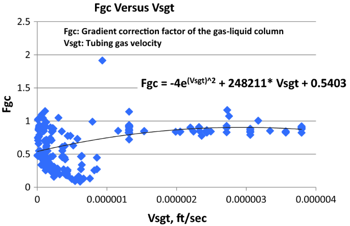
Gradient correction factor of the gaseous liquid column versus the tubing gas velocity
Fig. 2 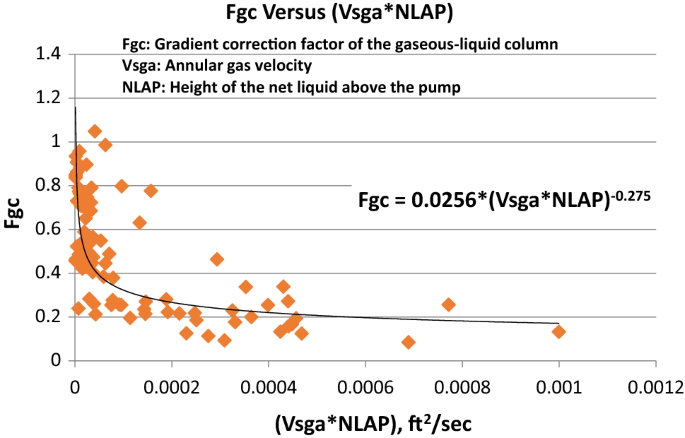
Gradient correction factor of the gaseous liquid column versus the annular gas velocity multiplied by the height of the net liquid above pump
- 6.
Using the relations shown in Figs. 1 and 2, two forms of new correlations were developed to calculate the gradient correction factor of the gaseous liquid column. The two correlations are presented as Eqs. 1 and 2.
$${\text{Fgc}} = - 4{\text{e}}^{{{\text{Vsgt}}^{2} }} + 248211 \times {\text{Vsgt}} + 0.54 03$$(1)$${\text{Fgc}} = 0.0256 \times \left( {{\text{Vsga }} \times {\text{NLAP}}} \right)^{0.275}$$(2)where \({\text{Fgc}}\) is the gradient correction factor of the gaseous liquid column; \({\text{Vsgt}}\) is the superficial gas velocity of the produced gas, ft/s; Vsga is the superficial gas velocity of the annular gas, ft/s; and NLAP is the height of the net liquid above the pump, ft


The first correlation is function of the tubing gas velocity, which can be calculated from the produced gas flow rate and tubing size. The second correlation, however, requires the annular gas velocity and the height of the net liquid above the pump. The annular gas velocity requirement means that the annular gas flow rate is measured.
- 7.
The first correlation was developed with 389 training data points. However, the second correlation was established by only 90 training data points because the second correlation required the availability of measured annular gas flow rate. Less data points were available with the measured annular gas flow rate. The 90 data points were common in the development of both the first and second correlations.
- 8.
The developed correlations were used to calculate the fluid gradient correction factor for the training data (389 data points for the first correlations and 90 data points for the second correlations). Then, the gaseous liquid column gradient and the PIP were calculated for all points.
- 9.
Other exiting methods (McCoy et al. 1988; Ghareeb et al. 2001) were used to compute PIP whenever possible for the training database (389 points). Depending on the availability of the required input data for McCoy et al. (1988) and Ghareeb et al. (2001), only 97 points and 100 points were used to calculate the PIP using the two methods, respectively. These calculations were carried out for comparison with the results of the newly proposed correlations.
- 10.
The two proposed correlations were validated using another 30 data points of actual field measurements (testing data).
Structure of the developed model
First correlation using tubing gas production rate
The first correlation depends on the tubing gas production rate, which is usually available in most pumped wells. This correlation needs only six input parameters: gas production rate, gas formation volume factor, wellhead tubing pressure, fluid level, downhole pump depth and surface oil (gas-free oil) specific gravity. The following five steps (Eqs. 3 to 7) detail the calculation of the PIP using this correlation:
- 1.
Calculate the estimated gas velocity from the measured tubing gas production rate
$${\text{Vsgt}} = 0.00167 *\left( {\frac{{q_{\text{g }} \times B_{\text{g}} }}{\text{At}}} \right)$$(3)where Vsgt is the superficial gas velocity of the produced gas, ft/s; qg is the gas production rate, MMscf/D; Βg is the gas formation volume factor, cf/scf; and At is the tubing cross-section area, in2
- 2.
Calculate the gradient correction factor of the gaseous liquid column
$${\text{Fgc}} = - 4{\text{e}}^{{\left( {\text{Vsgt}} \right)^{2} }} + 248211 \times {\text{Vsgt}} + 0.5403$$(4) - 3.
Calculate the gas-free oil gradient
$${\text{Go}} = 0.433 \times {\text{Yo}}$$(5)where Go is the oil gradient, psi/ft, and Yo is the specific gravity of oil
- 4.
Calculate the gaseous liquid column pressure
$${\text{Pglc}} = {\text{Fgc}} \times {\text{Go}} \times \left( {{\text{Dp}} - D_{\text{L}} } \right)$$(6)where Pglc is the pressure exerted by gaseous liquid column, psi; Dp is the pump depth, ft; and DL is the depth to top of liquid, ft
- 5.
Calculate the pump intake pressure
$${\text{PIP}} = {\text{Pt}} + {\text{Pglc}}$$(7)where PIP is the pump intake pressure, psi, and Pt is the tubing pressure, psi
This correlation was developed using 389 data points (training data) with MAPD of 25%. More points within the database were available to use this correlation because this correlation does not require casing pressure buildup rate or annular gas flow rate measurements.
Second correlation using annular gas rate
The second correlation is based on the annular gas flow rate. This correlation requires eight input parameters as follows: annular gas flow rate, gas formation volume factor, casing pressure, fluid level, downhole pump depth, surface oil (gas-free oil) specific gravity, casing inside diameter and tubing outside diameter. Using the annular gas flow rate, the following steps (Eqs. 8 to 12) are followed to calculate the PIP:
- 1.
Calculate the annular gas velocity from the annular gas rate
$${\text{Vsga}} = 0.00167 * \frac{{q_{\text{ga }} \times B_{\text{g}} }}{A}$$(8)where Vsga is the superficial gas velocity of the annular gas, ft/s; qga is the annular gas production rate, MMscf/D; Βg is the gas formation volume factor, cf/scf; and A is the annular cross-section area, in2
- 2.
Calculate the gradient correction factor of the gaseous liquid column
$${\text{Fgc}} = 0.0256 \times \left( {{\text{Vsga }} \times {\text{NLAP}}} \right)^{0.275}$$(9)where NLAP is the height of the net liquid above the pump, ft
- 3.
Calculate the gas-free oil gradient
$${\text{Go}} = 0.433 \times {\text{Yo}}$$(10)where Go is the oil gradient, psi/ft, and Yo is the specific gravity of oil
- 4.
Calculate the gaseous liquid column pressure
$${\text{Pglc}} = {\text{Fgc}} \times {\text{Go}} \times \left( {{\text{Dp}} - D_{\text{L}} } \right)$$(11)where Pglc is the pressure exerted by gaseous liquid column, psi; Dp is the pump depth, ft; and DL is the depth to top of liquid, ft
- 5.
Calculate the pump intake pressure
$${\text{PIP}} = {\text{Pgc}} + {\text{Pglc}} + {\text{Pc}}$$(12)where PIP is the pump intake pressure, psi; Pgc is the pressure exerted by gas column, psi; and Pc is the casing pressure, psi
This correlation was developed using only 90 training points (less data points were available with measured annular gas flow rate as it is not customary to measure the annular gas flow rate). This correlation showed MAPD of 20% using the training data.
Results for the training data
Figure 3 presents the MAPD between the measured and calculated PIPs with different calculation methods for the training data (389 points). It should be highlighted that the first correlation was developed from 389 points with MAPD of 25%. However, the second correlation was developed from only 90 points (less data points were available with measured annular gas rate). This correlation shows MAPD of 20%, which is less than the MAPD for the points (97 data points) that were applied with McCoy et al. method (its MAPD is 23%). However, the MAPD for the training points (100 data points) of Ghareeb et al. (2001) method was 44%.

MAPD between the measured and calculated PIPs with different calculation methods for the training datasets
Figure 3 shows also that if the PIP was calculated without taking the effect of the gas correction factor into consideration, the MAPD will reach 50%. The new correlations include new forms to calculate the fluid gradient correction factor, which enhance their accuracy.
Figure 4 presents the readings of the pressure sensors versus the corresponding calculated PIP of the different calculation methods for the training data. The deviation of the calculated PIP values from the measured pressures is shown with a 45° straight line.

Sensor readings versus the calculated PIP using different methods for training data
Model validation: results for testing data
Thirty testing data points were collected randomly from several oil fields to validate the model. These data are different from the data used for training to develop the new correlations. Table 3 shows the range of the testing data which were used to validate the two correlations.
The first correlation was verified using the 30 testing data points. However, only ten data points out of the 30 had measured annular gas flow rate, and therefore, were suitable for validating the second correlation. Also, only these ten data records included the required input data to calculate the PIP using McCoy et al. (1988) and Ghareeb et al. (2001) methods.
Validation of the first correlation
Table 4 summarizes the results of the absolute deviation between the calculated and measured PIPs for the 30 testing data points using the first correlation. As illustrated in Table 4, the MAPD between the calculated and measured PIPs is 33%.
Figure 5 is the graphical presentation of the calculated PIP using the first correlation against the actual PIP readings (blue squares). The deviation of the calculated PIP values from the measured pressures is shown with a 45-degree straight line.

Sensor readings versus the results of the first and second correlations for the testing data
Validation of the second correlation
Table 5 summarizes the results of the absolute deviation between the calculated and measured PIPs for the suitable ten testing data points using the second correlation method along with McCoy et al. (1988) and Ghareeb et al. (2001) methods.
As demonstrated in Table 5, the MAPD between the results of the second correlation against the corresponding sensors readings of the PIP is only 12%. Figure 5 presents also the relation between the measured PIP and the calculated values using the second correlation (red triangles). The deviation of the calculated PIP from the measured pressure is shown with a 45° straight line.
As shown in Table 5, the results of the second proposed correlation are better than those of the other models. For McCoy et al. (1988) method, the corresponding MAPD between the calculated and measured PIPs is 28% using the same testing data. In addition, the results of Ghareeb et al. (2001) method have higher MAPD than those of McCoy et al. (1988) method for these specific ten testing points. The MAPD between the calculated and the measured PIPs using Ghareeb et al. (2001) method is 61%.
Discussion
The results of the second correlation are more accurate than those of the first correlation and the other methods (McCoy et al. 1988; Ghareeb et al. 2001 methods). The first correlation needs only six input parameters (production rate, gas formation volume factor, wellhead tubing pressure, fluid level, downhole pump depth and surface oil (gas-free oil) specific gravity). These data are easily available and accessible in oil fields. However, the second proposed correlation is based on eight parameters including the annular gas production rate (annular gas flow rate, gas formation volume factor, casing pressure, fluid level, downhole pump depth, surface oil (gas-free oil) specific gravity, casing inside diameter and tubing outside diameter). The annular gas production rate may not be available in all cases. Similarly, Ghareeb et al. (2001) method requires the annular gas flow rate, but produces less accurate results. McCoy et al. (1988) method requires the measurement of casing buildup rate, which may not be available during the measurements of the DFL.
Neither annular gas production rate nor casing pressure buildup rate data are needed for the PIP calculations using the first proposed correlation. Therefore, the first proposed correlation has valuable role in the absence of annular gas flow rate measurements. In addition, the two proposed correlations can be applied in case no casing pressure buildup rate is available.
Both the first and second correlations can be used when the gas production rate (from the tubing) or annular gaseous flow rate is available, respectively. Having good estimate for the PIP will help in the following points:
- 1.
Understanding the well production capabilities
- 2.
Optimization of the artificial lift method that most fits the well according to the production capability
- 3.
Sizing the pump correctly. Oversizing the pump will consume more power and will decrease the pump run life. However, downsizing the pump will overload the equipment and will decrease the pump run life.
- 4.
Recalculation of the pump intake pressure regularly will help in optimizing the well, which will result in increasing the pump run life and optimizing the production and the well capital and operating expenses.
- 5.
PIP can be a factor to decide whether we need to switch from one artificial lift method to another.
- 6.
Optimizing the cost by running the low producer wells (sucker rod wells, plunger lift wells or progressive cavity pump wells) without sensors.
In some cases, large deviation between the calculated and the measured PIPs has been observed. This may be related to the following reasons (McCoy 1978):
- 1.
The accuracy of the PVT data (specially the oil formation volume factor) affects the calculations of the PIP.
- 2.
Stabilization of flow during the measurement of DFL has significant impact on the accuracy of the calculated bottom-hole flowing pressure and PIP. If the flow is not stable, the calculated values will be inaccurate.
- 3.
Height of the gaseous liquid column has impact on the calculated PIP. As the gaseous liquid column increases, the uncertainty in the bottom-hole flowing pressure and PIP increases.
- 4.
Accurate readings for the casing pressure and tubing head pressure are required. The accuracy of these gauges affects the calculations of bottom-hole flowing pressure and PIP.
- 5.
Annular gas flow rate should be measured accurately in the case of using correlations that require the annular flow rate as input.
Therefore, the above-mentioned concerns should be taken into consideration during the calculation procedures of the PIP to make sure that an accurate estimate for the PIP can be achieved.
Conclusions
-
1.
Two correlations were developed to correct the gaseous oil gradient and allow the estimation of the bottom-hole flowing pressure and PIP from DFL measurement and readily available data in the field.
-
2.
The two correlations were validated against actual measurements. The validation results showed reasonable accuracy.
-
3.
The first proposed correlation does not need the measurement of annular gas flow rate or casing pressure buildup rate measurement while taking the DFL reading. In this case, the PIP calculation will be easier and more efficient, especially for low-rate producers where downhole sensor data may not be warranted.
-
4.
The second proposed correlation does not need the casing pressure buildup rate measurement while taking the DFL measurement (similar to the first correlation). However, it needs the annular gas flow rate. If the annular gas flow rate is available, the second correlation is recommended to use for better accuracy.
Abbreviations
- A :
-
Annular cross-section area, in2
- At:
-
Tubing cross-section area, in2
- Β g :
-
Gas formation volume factor, cf/scf
- DFL:
-
Dynamic fluid level, ft
- D L :
-
Depth to top of liquid, ft
- Dp:
-
Pump depth, ft
- ESP:
-
Electrical submersible pump
- Fgc:
-
Gradient correction factor of the gaseous liquid column
- Go:
-
Oil gradient, psi/ft
- MAPD:
-
Mean absolute percentage deviation
- NLAP:
-
Height of the net liquid above the pump, ft
- Pc:
-
Casing pressure, psig
- Pgc:
-
Pressure exerted by gas column, psi
- Pglc:
-
Pressure exerted by gaseous liquid column, psi
- PIP:
-
Pump intake pressure, psi
- Pt:
-
Tubing pressure, psi
- q g :
-
Gas production rate, MMscf/D
- q ga :
-
Annular gas production rate, MMscf/D
- \({\text{Vsga}}\) :
-
Superficial gas velocity of the annular gas, ft/s
- \({\text{Vsgt}}\) :
-
Superficial gas velocity of the produced gas, ft/s
- Yo:
-
Specific gravity of oil
- ∆P/∆t :
-
Pressure buildup data, psi/min
References
Burgstaller C (2016) New approaches of using fluid level data for production optimization and reservoir engineering applications. In: SPE-180159-MS, SPE Europec 78th EAGE Conference and Exhibition, Vienna, 30 May–2 June 2016
Ghareeb M, Shalaby SE, Elayouty ED, Soleiman MM, Tantawy MA (2001) New correlation for predicting the gradient of gaseous-liquid column in the casing-tubing annulus for pumped wells. In: 4th Syrian–Egyptian conference, Damascus, pp 585–602, 9–11 October 2001
Hasan AR, Kabir CS (1985) Determining bottomhole pressures in pumping wells. SPE J 25(6):823–838 (SPE paper 11580-PA)
McCoy JN (1978) Determining producing bottom hole pressure in wells having gaseous columns. JPT 30(1):117–119 (SPE paper 6476-PA)
McCoy JN, Podio AL, Huddleston KL (1988) Acoustic determination of producing bottomhole pressure. In: SPE paper 14254, presented at the SPE 1988 annual technical conference and exhibition, Las Vegas
Nind TEW (1969) Principles of oil well production. McGraw-Hill Book Co., Inc., NY
Podio AL, Tarrillion MJ, Roberts ET (1980) Bottom hole pressure method and correlations are reviewed. Oil Gas J 18:79–83
Rowlan OL, McCoy JN, Podio AL (2011) Pump intake pressure determined from fluid levels, dynamometers, and valve-test measurements. J Can Pet Technol 50(4):59–67 (SPE paper 142862-PA)
Walker CP (1936) Determination of fluid level in oil wells by the pressure-wave echo method. In: Los Angeles meeting, October, 1936, Transactions of AIME
Author information
Authors and Affiliations
Corresponding author
Additional information
Publisher's Note
Springer Nature remains neutral with regard to jurisdictional claims in published maps and institutional affiliations.
Rights and permissions
Open Access This article is licensed under a Creative Commons Attribution 4.0 International License, which permits use, sharing, adaptation, distribution and reproduction in any medium or format, as long as you give appropriate credit to the original author(s) and the source, provide a link to the Creative Commons licence, and indicate if changes were made. The images or other third party material in this article are included in the article's Creative Commons licence, unless indicated otherwise in a credit line to the material. If material is not included in the article's Creative Commons licence and your intended use is not permitted by statutory regulation or exceeds the permitted use, you will need to obtain permission directly from the copyright holder. To view a copy of this licence, visit http://creativecommons.org/licenses/by/4.0/.
About this article

Cite this article
El-Saghier, R.M., Abu El Ela, M. & El-Banbi, A. A model for calculating bottom-hole pressure from simple surface data in pumped wells. J Petrol Explor Prod Technol 10, 2069–2077 (2020). https://doi.org/10.1007/s13202-020-00855-y
Received:
Accepted:
Published:
Issue Date:
DOI: https://doi.org/10.1007/s13202-020-00855-y