
Abstract
A layered partial-consensus fuzzy collaborative forecasting approach is proposed in this study to forecast the unit cost of a dynamic random access memory (DRAM) product. In the layered partial-consensus fuzzy collaborative forecasting approach, the partial-consensus fuzzy intersection (PCFI) operator is applied instead of the prevalent fuzzy intersection (FI) operator to aggregate the fuzzy forecasts by experts. In this way, some meaningful information, such as the suitable number of experts, can be obtained through observing changes in the PCFI result when the number of experts varies. After applying the layered partial-consensus fuzzy collaborative forecasting approach to a real case, the experimental results revealed that the layered partial-consensus fuzzy collaborative forecasting approach outperformed three existing methods. The most significant advantage was up to 13%.
Introduction
Fuzzy collaborative forecasting is the combination of fuzzy forecasting [28] and collaborative intelligence [18, 25]. In a fuzzy collaborative forecasting approach, multiple experts apply various fuzzy forecasting methods to forecast a target and collaborate by consulting each other’s forecast so as to modify their fuzzy forecasting methods or forecasts [13]. Unlike conventional forecasting methods that are focused on optimizing the forecasting accuracy, a fuzzy collaborative forecasting approach attempts to optimize both the forecasting precision and accuracy [12].
In this study, the unit cost of a dynamic random access memory (DRAM) product is to be forecasted. The unit cost of a DRAM product is a special time series [11]. For this reason, some recent references on fuzzy time series forecasting are reviewed as follows. To forecast the weighted stock index, Wong et al. [43] applied fuzzy inference rules. According to the forecasting accuracy, the input space was redivided by adjusting the window size. Egrioglu et al. [21] applied fuzzy c-means (FCM) and an artificial neural network (ANN) jointly to forecast the enrollment result of University of Alabama. First, FCM was applied to fuzzify historical data. Subsequently, the fuzzification results became inputs to an ANN that forecasted the enrollment result. Cai et al. [4] established a fuzzy autoregression model to forecast the weighted stock index. Ant colony optimization (ACO) was applied to optimize the fuzzification of the antecedents of the fuzzy autoregression model. Cheng et al. [19] constructed a fuzzy inferencing system to forecast the weighted stock index. They applied particle swarm optimization (PSO) to optimize the division of the input space, and K-means to determine the center of a fuzzy antecedent. Singh and Dhiman [34] proposed the geese movement-based optimization algorithm (GMBOA) to optimize the fuzzification of inputs to fuzzy inference rules applied to forecast the stock index. However, these methods are not readily applicable to forecast the unit cost of a DRAM product that improves according to a learning process [11]. Soto et al. [37] applied the ensemble of a fuzzy inference system (FIS) and an adaptive-network-based fuzzy inference system (ANFIS) to forecast several stock indexes. There are also fuzzy time series forecasting methods based on other types of fuzzy sets, such as type II fuzzy sets [29, 35, 36], hesitant fuzzy sets [3], and others.
The proposed methodology is a fuzzy collaborative forecasting method. Therefore, some references on fuzzy collaborative forecasting are also reviewed. In Cheikhrouhou et al. [6], an autoregressive integrated moving average (ARIMA) model was built to forecast the demand for polyethylene bags. Subsequently, experts made their judgments on the effects of unexpected future events on demand. Such judgments determined changes that were made to the forecasts [2]. Fuzzy inference systems (FISs), such as Mamdani’s FISs, Sugeno’s FISs [24], and ANFISs [33], etc., apply multiple fuzzy inference rules that cannot guarantee the inclusion of actual values in the corresponding fuzzy forecasts [12]. Chen [7] proposed a fuzzy collaborative forecasting method in which each expert fitted a fuzzy linear regression (FLR) equation to predict the effective cost per die of a DRAM product. The values of fuzzy parameters in the FLR equation were derived by solving nonlinear programming problems. In this way, all actual values were contained in the corresponding fuzzy forecasts, at least for the training data. Subsequently, fuzzy intersection (FI), or the minimum T-norm, was applied to aggregate the fuzzy forecasts by all experts, which optimized the forecasting precision in terms of the average range of fuzzy forecasts. After that, a back propagation network (BPN) was constructed to defuzzify the aggregation result, so as to optimize the forecasting accuracy measured with the root mean squared error (RMSE). Similar fuzzy collaborative forecasting methods have been proposed in subsequent studies for forecasting the cycle time of a job [9], the unit cost of a DRAM product [11], etc. Zarandi et al. [44] established a four-layer fuzzy multiagent system (FMAS) to forecast the next-day stock price based on the collaboration among software agents. In the fuzzy collaborative forecasting methods proposed by Chen and Wang [17] and Chen and Romanowski [15], software agents, instead of real experts, were also used to expedite the collaboration process. However, when the values of fuzzy parameters in a fuzzy forecasting method need to be adjusted, software agents usually follow pre-specified rules, which may result in unrealistic fuzzy forecasts. Chen [10] proposed a heterogeneous fuzzy collaborative forecasting approach to predict the yield of a semiconductor product, in which experts fitted the yield learning process of the product with FLR equations by solving mathematical planning problems or training an ANN. Lin and Chen [25] proposed a fuzzy collaborative forecasting approach that was able to deal with the original value, rather than the logarithmic or log-sigmoid value, of a target that improved according to a fuzzy learning process. In the view of Chen and Honda [12], a fuzzy analytic hierarchy process problem can be considered as an unsupervised fuzzy collaborative forecasting problem. A major difference between fuzzy collaborative forecasting methods and fuzzy time series forecasting methods is that the former improves the forecasting accuracy by tuning the fuzzification mechanism, while, the latter optimizes the defuzzification mechanism to achieve the same purpose [4, 13].
A layered partial-consensus fuzzy collaborative forecasting approach is proposed in this study to forecast the unit cost of a DRAM product. The motives are explained as follows.
-
(1)
In most existing fuzzy collaborative forecasting methods, FI is applied to aggregate the fuzzy forecasts by experts. The FI result usually covers a very narrow range. The possibility of missing an actual value is high for test (unlearned) data.
-
(2)
An existing fuzzy collaborative forecasting method considers the fuzzy forecasts by all experts. As a result, the aggregation result is subject to the forecast by a radical expert.
-
(3)
When the overall consensus among all experts does not exist, the FI operator is not applicable.
To overcome these drawbacks, the consensus among some experts, rather than all experts, can be sought for instead. To this end, Chen [8] proposed the concept of a partial-consensus FI (PCFI) operator. The PCFI result is not a null set if some experts can achieve a (partial) consensus. As a result, the PFCI result covers a wider range than FI does, thereby decreasing the possibility of missing an actual value for test data. In addition, through observing changes in the PCFI result when the number of experts varies, some meaningful information can be obtained. From this point of view, the concept of the layered PCFI (LPCFI) diagram is presented in this study, based on which the layered partial-consensus fuzzy collaborative forecasting approach is proposed.
The originality of the proposed methodology resides in the following aspects:
-
(1)
Unlike most existing fuzzy collaborative forecasting methods, the proposed methodology seeks for the consensus among some experts, rather than that among all experts, so as to increase the possibility of reaching a consensus.
-
(2)
Chen [8] also sought for the partial consensus among some of the experts. However, how to determine the number of experts among whom the consensus is sought for is an unsolved issue. The LPCFI diagram presented in this study provides a viable means of determining the suitable number of experts for a fuzzy collaborative forecasting task.
The contribution of this study includes.
-
(1)
The establishment of a systematic procedure for determining the suitable number of experts under a fuzzy collaborative forecasting environment, and
-
(2)
The design of an effective mechanism for controlling the range of a fuzzy forecast so that actual value can be included in the fuzzy forecast.
The remainder of this paper is organized as follows. Section 2 is a preliminary about the steps of a fuzzy collaborative forecasting approach. Section 3 presents the concept of the LPCFI diagram, and introduces the layered partial-consensus fuzzy collaborative forecasting approach. Section 4 describes the case of forecasting the unit cost of a DRAM product for illustrating the applicability of the layered partial-consensus fuzzy collaborative forecasting approach. Some existing methods were also applied to the case for comparison. Section 5 concludes this study and puts forth some topics for future investigation.
Preliminary
Without loss of generality, all fuzzy parameters and variables in this study are given in or approximated with triangular fuzzy numbers (TFNs) [23].
According to Chen and Honda [13], the application procedure of a fuzzy collaborative forecasting approach comprises seven steps:
Step 1. (Each expert) Apply a fuzzy forecasting method to make a fuzzy forecast of the same target.
Step 2. Aggregate the fuzzy forecasts by all experts.
Step 3. Defuzzify the aggregation result to arrive at a representative/crisp value.
Step 4. Evaluate the forecasting performance, including the forecasting precision and accuracy.
Step 5. If the forecasting performance is satisfactory, go to Step 7; otherwise, go to Step 6.
Step 6. (Each expert) Modify the fuzzy forecast by consulting others’ fuzzy forecasts. Return to Step 2.
Step 7. End.
The procedure is illustrated in Fig. 1. The steps are described in the following.

The procedure of a fuzzy collaborative forecasting approach
Making a fuzzy forecast
In a fuzzy collaborative forecasting approach, each expert applies a fuzzy forecasting method to forecast a target y from decision variables {xi}, e.g.,
where (+) denotes fuzzy addition. However, even if all experts apply the same fuzzy forecasting method, the values of fuzzy parameters in the fuzzy forecasting method are different. As a result, the fuzzy forecasts by experts are not the same and need to be aggregated.
Some ways to derive the values of fuzzy parameters in Eq. (1) are reviewed as follows. Tanaka and Watada [39] proposed a linear programming (LP) method to minimize the sum of the ranges (or spreads) of fuzzy forecasts, so as to maximize the forecasting precision. Taheri and Kelkinnama [38] solved another LP problem to minimize the sum of absolute errors. Peters [30] proposed a quadratic programming (QP) method, which maximizes the average satisfaction level to optimize the forecasting accuracy. Optimizing the forecasting accuracy and precision at the same time has been pursued by all researchers, but is a challenging task. To address this, a compromise approach was proposed by Donoso et al. [20] by minimizing the weighted sum of two objective functions: the sum of the squared deviations between the cores of fuzzy forecasts and actual values, and the sum of the squared ranges.
Chen and Lin [14] incorporated an expert’s opinions into the model of Tanaka and Watada [39] and that of Peters [30], and proposed two nonlinear programming (NLP) models as.
(NLP Model I)
subject to
The objective function is to minimize the power sum of the ranges (or spreads) of fuzzy forecasts. o ≥ 0. The value of o reflects the sensitivity of an expert to the uncertainty in fuzzy forecasts: from small (not sensitive) to large (very sensitive). Constraints (3) and (4) ensure that the membership of an actual value in the corresponding fuzzy forecast is equal to or greater than a pre-specified threshold s. Equations (5–7) make a fuzzy forecast. Constraints (8) and (9) define the sequence of corners in a TFN parameter.
In Model NLP I, if o is a large value, it becomes difficult to optimize the NLP problem. For this reason, Chen and Wang [17] advised to choose the value of o from [0, 4]. When o is a positive integer, the model can be converted into an equivalent QP model. Otherwise, Chen and Wang [16] proposed a method to approximate the model with a QP one. First, the value of yj is normalized into [0, 1]:
As a result,
since \( y_{{j3}} \ge y_{{j1}} \). Chen and Wang’s method approximated the objective function with a quadratic equation. For example, when o = 1.5,
(NLP Model II)
subject to
The objective function is to maximize the power sum of the satisfaction levels. m ≥ 0. The value of m reflects the sensitivity of an expert to the improvement in the satisfaction level: from small (not sensitive) to large (very sensitive). Constraint (14) restricts the generalized mean of the ranges. When o and m are both positive integers, the model can be converted into an equivalent QP model. Otherwise, Chen and Wang’s method can also be applied to approximate the model with a QP one in a similar way.
Aggregating the fuzzy forecasts by experts
The FI operator is the most common method for aggregating the fuzzy forecasts by all experts in existing fuzzy collaborative forecasting approaches [12, 27, 41]:
which membership function can be derived byapplying the minimum t-norm [14]:
If the fuzzy forecast by each expert includes an actual value, then the FI result also includes the actual value, at least for the training (or learned) data. Otherwise, fuzzy union (i.e., the maximum t-conorm or s-norm) should be applied instead, such as the treatment taken in existing FISs.
FI finds out values common to the fuzzy forecasts by all experts. Therefore, the FI result can be used to represent the overall consensus among experts. When the fuzzy forecast by each expert is represented by a TFN, the FI result is a polygonal fuzzy number (see Fig. 2, and its α cut can be derived as
where \([\tilde{y}_{j}^{L} (k)(\alpha ),\;\tilde{y}_{j}^{R} (k)(\alpha )]\) is the α cut of \(\tilde{y}_{j} (k)\).

The FI result
When the overall consensus among experts does not exist, the FI result is a null set. In such a situation, the consensus among some experts can be sought for instead. To this end, Chen [8] proposed the concept of the PCFI operator.
Definition 1.
The H/K PCFI result of the fuzzy forecasts by K experts at period j, i.e., \(\tilde{y}_{j} (1)\) ~ \(\tilde{y}_{j} (K)\), is indicated with \(\widetilde{PCFI}^{H/K} (\{ \tilde{y}_{j} (k)\} )\) such that.
where h = 1 ~ H; H ≥ 2; g() = 1 ~ K; g(p) ∩ g(q) = ∅ ∀ p ≠ q. By applying the minimum t-norm and s-norm to deal with the intersection and union operations, respectively,
From the managerial point of view, in PCFI, fuzzy intersection and fuzzy union are applied for handling parts with and without consensus, respectively.
For example, the 2/3 PCFI result of \(\tilde{y}_{i} (1)\) ~ \(\tilde{y}_{i} (K)\) can be derived as
which is illustrated in Fig. 3.

The PCFI result
A FI operator meets four requirements: boundary conditions, monotonicity, commutativity, and associativity. A fuzzy union operator also meets the same requirements. However, the boundary conditions for a FI operator are contradictory to those for a fuzzy union operator. Therefore, a PCFI operator meets three requirements: monotonicity, commutativity, and associativity.
Defuzzifying the aggregation result
In existing fuzzy forecasting methods, a BPN is usually constructed to defuzzify the aggregation result with the following configuration, [13, 40]:
-
(1)
Input: Inputs to the BPN are the value and membership of each corner of the aggregation result.
-
(2)
A single hidden layer: The number of nodes in the hidden layer is equal to that of inputs.
-
(3)
Output: the forecast.
-
(4)
The training algorithm: The gradient descent (GD) algorithm and the Levenberg–Marquardt (LM) algorithm are two prevalent training algorithms for this purpose [8, 40].
-
(5)
Convergence criteria: The training process stops when the sum of squared error (SSE) falls below a pre-specified threshold,
$$ SSE = \sum\limits_{j = 1}^{n} {(y_{j} - o_{j} )^{2} } , $$(30)
or a maximal number of epochs have been run.
The proposed methodology
A LPCFI diagram
The PCFI result changes when the number of experts varies, as illustrated in Fig. 4.

Changes in the PCFI result as the number of experts varies
By observing changes in the PCFI result, some meaningful information can be obtained. From this point of view, the concept of the LPCFI diagram is presented as follows.
Definition 2.
A LPCFI diagram is a systematic representation of changes in the partial consensus among multiple experts (i.e., \(\widetilde{PCFI}^{H/K}\)) when the number of experts (i.e., H) varies.
An example is provided in Fig. 5.

A LPCFI diagram
In the LPCFI diagram,
-
(1)
Obviously, \(\widetilde{PCFI}^{2/4} \supset \widetilde{PCFI}^{3/4} \supset \widetilde{PCFI}^{4/4}\).
-
(2)
If the consensus among more experts is sought for, the aggregation result is a narower range. A narrower range means a higher forecasting precision for the training data, but may increase the possibility of missing an actual value for test data.
-
(3)
By contrast, it is easier to seek for the conensus among fewer experts. The aggregation result covers a wider range.
In existing fuzzy collaborative forecasting methods, the narrowest aggregation result is usually sought for to maximize the forecasting precision. However, the future situation may be quite different from that in the past, adopting the narrowest aggregation result is risky. As an alternative, a wider aggregation result can be adopted.
The LPCFI diagram can be consulted to determine the suitable number of experts that reach a consensus. Taking the LPCFI diagram in Fig. 6 as an example. The consensus among four experts does not exist, while that between three experts exists but the aggregation result is too narrow. If the future condition may be much different from the past, then seeking for the partial consensus between two experts is less risky. Therefore, the suitable number of experts may be two. Namely, four experts are gathered to collect diversified fuzzy forecasts, but it is acceptable if only two of them reach a consensus.

An example of determining the suitable number of experts
It is always better to seek for the consensus among more experts, if which is not risky. Another example is given in Fig. 7. It can be seen that \(\widetilde{PCFI}^{3/4} \approx \widetilde{PCFI}^{4/4}\), implying that seeking for the consensus among only three experts is not less risky than that among four experts. In this case, the suitable number of experts is four.

Another example of determining the suitable number of experts
A BPN for defuzzifying the aggregation result
The BPN for defuzzifying the aggregation result in terms of \(\widetilde{PCFI}^{H/K}\) is denoted with \({\text{BPN}}^{H/K}\). Undoubtedly, the BPN defuzzifiers for different PCFI results are not the same. Namely, \({\text{BPN}}^{{H_{1} /K}} \ne {\text{BPN}}^{{H_{2} /K}}\) if \(H_{1} \ne H_{2}\). The configuration of the BPN defuzzifier is as follows:
-
(1)
Input: Accordng to Fig. 7, it is obvious that a lower value of H results in a polygonal fuzzy number with more corners, which means more inputs to the BPN defuzzifier. As a consequence, the corners of the PCFI result may be numerous. To address this issue, only the values and memberships of some representative corners of the PCFI result are chosen as inputs to the BPN. Such representative corners include the leftmost and rightmost corners and the corners with the highest memberships. Taking Fig. 8 as an example. The five representative corners are marked with circles in this figure. As a result, the number of inputs to the BPN is ten.
Fig. 8 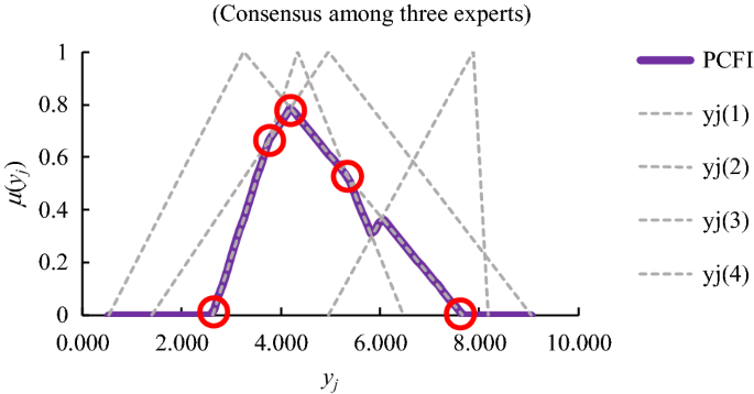
Choosing inputs to the BPN
-
(2)
A single hidden layer: The number of nodes in the hidden layer is equal to that of inputs.
-
(3)
Output: \(o_{j}\), to be compared with \(y_{j}\).
-
(4)
The training algorithm: the GD algorithm to prevent overfitting [40].
-
(5)
Convergence criteria: The training process stops when SSE falls below 10–4 or a maximal number of 1000 epochs have been run.

Application—Forecasting the unit cost of a DRAM product
Background
The proposed methodology has been applied to forecast the unit cost of a DRAM product [7], for which the unit cost was forecasted by fitting a FLR equation in various ways. Four experts applied Chen and Lin’s NLP methods to derive the values of fuzzy parameters in the FLR equation:
Expert #1: NLP Model I; o = 1; s = 0.5
Expert #2: NLP Model I; o = 3; s = 0.35.
Expert #3: NLP Model II; o = 2; m = 2; d = 1.73.
Expert #4: NLP Model II; o = 1; m = 3; d = 1.82.
Lingo 16.0 × 64 was applied to build the NLP models and implement a branch-and-bound algorithm to solve the NLP problems on a PC with Intel Core i7-7700 CPU 3.60 GHz and 8 GB RAM. These NLP models were coded and optimized using Lingo. The NLP model of Expert #3 is illustrated in Fig. 9.

The NLP model of Expert #3
The unit cost data were split into two parts: the data of the first six periods for building the models, and the remaining data for testing. The forecasting results by experts are shown in Fig. 10.

The forecasting results by experts
The fuzzy forecasts by experts were defuzzified using the center-of-gravity (COG) method. Then, the forecasting performance without collaboration was evaluated in terms of mean absolute error (MAE), mean absolute percentage error (MAPE), and RMSE. The results are summarized in Table 1.
Application of the proposed methodology
To improve the forecasting performance, the layered partial-consensus fuzzy collaborative forecasting approach was applied. First, taking the forecasts by experts at period 3 as an example. The LPCFI diagram is shown in Fig. 11. The following phenomena were observed:
-
(1)
By adding one more expert, the aggregation result among experts shrank very rapidly.
-
(2)
The aggregation result among all experts fell within a very narrow range.

The LPCFI diagram at period 3
The aggregation result by seeking for the consensus between two experts was too wide, while that among four experts was too narrow, as depicted in Table 2. A reasonable choice was, therefore, to seek for the consensus among three experts.
\(\widetilde{PCFI}^{{{3}/4}}\) was applied to aggregate the fuzzy forecasts by experts. The aggregation results are shown in Fig. 12. All actual values in test data fell within the corresponding aggregation results, showing the effectiveness of the proposed methodology.

The aggregation results
Subsequently, the aggregation result was defuzzified using a BPN. For this purpose, first, the five representative corners of the aggregation result at each period were found out. The results are summarized in Table 3. As a result, the number of inputs to the BPN defuzzifier was ten. The number of nodes in the hidden layer was set to ten as well. The BPN was trained using the GD algorithm to prevent overfitting. The convergence criteria were established as follows:
-
(1)
SSE < 10–4;
-
(2)
1000 epochs have been run.
The BPN defuzzifier was implemented using the neural network toolbox of MATLAB 2017 on a PC with i7-7700 CPU 3.6 GHz and 8 GB RAM. The program codes are illustrated in Fig. 13. The execution time was less than 1 s. The defuzzification results are shown in Fig. 14.

The problem codes of the BPN defuzzifier

The defuzzification results
The forecasting accuracy using the layered partial-consensus fuzzy collaborative forecasting approach was evaluated as.
MAE = 0.076,
MAPE = 4.83%,
RMSE = 0.134.
Compared with existing methods
For comparison, three existing methods were applied to the case as well. The first method is the 6σ logistic regression method that fitted the collected unit cost data with the following logistic regression model:
with σ = 0.126. The upper bound (or lower bound) on a forecast was established by adding 3σ to (or subtracting 3σ from) the forecast. The results are shown in Fig. 15. The forecasting accuracy using the 6σ logistic regression method was evaluated as.

The forecasting results using the 6σ logistic regression method
MAE = 0.118,
MAPE = 7.75%,
RMSE = 0.177.
The forecasting performance was poorer than those by some experts without collaboration, which revealed the superiority of a fuzzy forecasting method.
Subsequently, the fuzzy collaborative forecasting method proposed by Chen [7] was also applied, in which the overall consensus among all experts was sought for. The aggregation results are shown in Fig. 16. An actual value in test data was missed. The forecasting accuracy using the fuzzy collaborative forecasting method was evaluated as.

The forecasting results using the fuzzy collaborative forecasting method proposed by Chen [7]
MAE = 0.088,
MAPE = 5.68%,
RMSE = 0.142,
which was poorer than that using the proposed methodology.
The third existing method compared in the experiment was the direct-solving fuzzy collaborative forecasting method proposed by Lin and Chen [25], in which the followng formula was applied to approximate the exponential function for building the fuzzy learning model of the unit cost:
As a result, experts solved polynomial programming (PP) problems instead to made fuzzy forecasts. Then, the FI operator and a BPN were applied to aggregate the fuzzy forecasts by experts and defuzzify the aggregation result, respectively. The forecasting performance using the direct-solving fuzzy collaborative forecasting method was evaluated as.
MAE = 0.085,
MAPE = 5.54%,
RMSE = 0.135.
A summary of the forecasting performances of various methods is provided in Fig. 17. According to the experimental results,
-
(1)
After experts’ collaboration, the forecasting performance, especially the forecasting accuracy, was elevated.
-
(2)
Obviously, the proposed layered partial-consensus fuzzy collaborative forecasting approach surpassed all existing methods compared in the experiment.
-
(3)
The proposed methodology had the most significant advantage over existing methods in reducing MAPE, which was up to 13%.
-
(4)
A paired t test was conducted to see whether the advantage of the proposed methodology over existing methods was significant or not:

A summary of the forecasting performances of various methods
H0: When improving the forecasting accuracy in terms of the absolute error, the performance of the proposed methodology is the same as that of the existing method.
H1: When improving the forecasting accuracy in terms of the absolute error, the performance of the proposed methodology is more effective than that of the compared existing method.
The results are summarized in Table 4. The forecasting accuracy of the proposed methodology was statistically better than those of 6σ logistic regression and Chen [7] when α = 0.05.
-
(5)
To further elaborate the effectiveness of the proposed methodology, it was applied to another case that contained the unit cost data of another DRAM product within 12 periods. The unit cost data within the first six periods were used to build the models, while the remaining data were reserved for evaluating the forecasting performance. A group of three experts was formed to forecast the unit cost of the DRAM product collaboratively. The models chosen by the experts were
Expert I: NLP Model II (\( o(1) = {{1}} \), \( m(1) = {{3}} \), \( d(1) = 0.{{72}} \)).
Expert II: NLP Model I (\( o(2) = 2 \), \( s(2) = 0.{{33}} \)).
Expert III: NLP Model II (\( o(1) = {{3}} \), \( m(1) = {{2}} \), \( d(1) = 0.{{6}}4 \)).
The LPCFI diagram at period 6 is presented in Fig 18. Obviously, when the consensus between three experts was sought for, the aggregation result covered a very narrow range, which might be risky for responding to unexpected future conditions. For this reason, the partial consensus between two experts was sought for instead. The aggregation results at all periods are summarized in Fig. 19. After defuzzifying the aggregation result using a BPN, the forecasting results are shown in Fig. 20. The forecasting accuracy was evaluated as follows:

The LPCFI result at period 6

The aggregation results

The forecasting results
MAE = 0.039,
MAPE = 2.77%,
MAPE = 0.045.
which showed a very good fit that supported the effectiveness of the proposed methodology.
Conclusions
Fuzzy collaborative forecasting methods have great potential to enhance both the forecasting precision and accuracy. However, most existing fuzzy collaborative forecasting methods apply the FI operator to aggregate the fuzzy forecasts by experts, which is subjected to several drawbacks. To overcome these drawbacks, the PCFI operator proposed by Chen [8] is useful. In addition, some meaningful information, such as the suitable number of experts, can be obtained through observing changes in the PCFI result when the number of experts varies. From this point of view, the concept of the LPCFI diagram is proposed in this study, based on which the layered partial-consensus fuzzy collaborative forecasting approach is proposed. The layered partial-consensus fuzzy collaborative forecasting approach reduces the risk of missing an actual value when future conditions are considerably different from those in the past.
The layered partial-consensus fuzzy collaborative forecasting approach and three existing methods have been applied to forecast the unit cost of a DRAM product for comparison. According to the experimental results, the following conclusions were drawn:
-
(1)
The forecasting accuracy achieved using the layered partial-consensus fuzzy collaborative forecasting approach, in terms of MAE, MAPE, or RMSE, was superior to those of the three existing methods. The layered partial-consensus fuzzy collaborative forecasting approach had the most significant advantage over existing methods when MAPE was minimized, which was up to 13% on average.
-
(2)
The forecasting accuracy improved after experts’ collaboration.
-
(3)
By determining the suitable number of experts, the layered partial-consensus fuzzy collaborative forecasting approach effectively reduced the risk of missing an actual value. The hit rate for test data was up to 100%.
-
(4)
In the three fuzzy collaborative forecasting methods, only the layered partial-consensus fuzzy collaborative forecasting approach achieved a hit rate of 100%, which also contributed to its superiority in optimizing the forecasting accuracy since no actual value was missed.
In future studies, advanced algorithms can be applied to solve the NLP problems [1, 5, 32]. In addition, the number of experts may vary for different purposes, e.g., the partial consensus between two experts for estimating the range of the unit cost, while that among three experts for forecasting the unit cost. Further, the layered partial-consensus fuzzy collaborative forecasting approach is a general methodology that can be applied to other forecasting tasks in various fields [22, 26, 31, 42]. Furthermore, the situation in which experts have unequal influences on the forecasting result needs to be investigated. These constitute some directions for future research.
References
Abed-alguni BH (2019) Island-based cuckoo search with highly disruptive polynomial mutation. Int J Artif Intell 17(1):57–82
Amindoust A, Ahmed S, Saghafinia A, Bahreininejad A (2012) Sustainable supplier selection: a ranking model based on fuzzy inference system. Appl Soft Comput 12(6):1668–1677
Bisht K, Kumar S (2016) Fuzzy time series forecasting method based on hesitant fuzzy sets. Expert Syst Appl 64:557–568
Cai Q, Zhang D, Zheng W, Leung SC (2015) A new fuzzy time series forecasting model combined with ant colony optimization and auto-regression. Knowl-Based Syst 74:61–68
Castillo O, Valdez F, Melin P (2007) Hierarchical Genetic Algorithms for topology optimization in fuzzy control systems. Int J Gen Syst 36(5):575–591
Cheikhrouhou N, Marmier F, Ayadi O, Wieser P (2011) A collaborative demand forecasting process with event-based fuzzy judgements. Comput Ind Eng 61(2):409–421
Chen T (2011) Applying the hybrid fuzzy c-means-back propagation network approach to forecast the effective cost per die of a semiconductor product. Comput Ind Eng 61(3):752–759
Chen T (2012) A hybrid fuzzy and neural approach with virtual experts and partial consensus for DRAM price forecasting. Int J Innov Comput Inform Control 8(1):583–597
Chen T (2013) An effective fuzzy collaborative forecasting approach for predicting the job cycle time in wafer fabrication. Comput Ind Eng 66(4):834–848
Chen T (2017) An ANN approach for modeling the multisource yield learning process with semiconductor manufacturing as an example. Comput Ind Eng 87:296–307
Chen T, Chiu MC (2015) An improved fuzzy collaborative system for predicting the unit cost of a DRAM product. Int J Intell Syst 30(6):707–730
Chen TCT, Honda K (2019) Fuzzy collaborative forecasting and clustering: methodology, system architecture, and applications. Springer, Switzerland AG
Chen TCT, Honda K (2020) Nonlinear fuzzy collaborative forecasting methods. Fuzzy Collab Forecast Clust, pp 27–44
Chen T, Lin YC (2008) A fuzzy-neural system incorporating unequally important expert opinions for semiconductor yield forecasting. Int J Uncertain Fuzziness Knowl-Based Syst 16(1):35–58
Chen T, Romanowski R (2014) Forecasting the productivity of a virtual enterprise by agent-based fuzzy collaborative intelligence – with Facebook as an example. Appl Soft Comput 24:511–521
Chen T, Wang YC (2013) Semiconductor yield forecasting using quadratic-programming-based fuzzy collaborative intelligence approach. Math Probl Eng 672404:1–7
Chen T, Wang YC (2014) An agent-based fuzzy collaborative intelligence approach for precise and accurate semiconductor yield forecasting. IEEE Trans Fuzzy Syst 22(1):201–211
Chen J, Zhao C, Chen L (2019) Collaborative filtering recommendation algorithm based on user correlation and evolutionary clustering. Compl Intell Syst 1–10
Cheng SH, Chen SM, Jian WS (2016) Fuzzy time series forecasting based on fuzzy logical relationships and similarity measures. Inf Sci 327:272–287
Donoso S, Marín N, Vila MA (2006) Quadratic programming models for fuzzy regression. Proceedings of international conference on mathematical and statistical modeling in honor of Enrique Castillo.
Egrioglu E, Aladag CH, Yolcu U (2013) Fuzzy time series forecasting with a novel hybrid approach combining fuzzy c-means and neural networks. Expert Syst Appl 40(3):854–857
Gil RA, Johanyák ZC, Kovács T (2018) Surrogate model based optimization of traffic lights cycles and green period ratios using microscopic simulation and fuzzy rule interpolation. Int J Artif Intell 16(1):20–40
Huang D, Chen T, Wang MJJ (2001) A fuzzy set approach for event tree analysis. Fuzzy Sets Syst 118(1):153–165
Kaur A, Kaur A (2012) Comparison of mamdani-type and sugeno-type fuzzy inference systems for air conditioning system. Int J Soft Comput Eng 2(2):323–325
Lin YC, Chen T (2019) An advanced fuzzy collaborative intelligence approach for fitting the uncertain unit cost learning process. Compl Intell Syst 5(3):303–313
Lin YC, Chen T, Wang YC (2013) A fuzzy collaborative sensor network for semiconductor manufacturing cycle time forecasting. Int J Distrib Sens Netw 9(3):257276
Lin YC, Wang YC, Chen TCT, Lin HF (2019) Evaluating the suitability of a smart technology application for fall detection using a fuzzy collaborative intelligence approach. Mathematics 7(11):1097
Marcek D (2018) Forecasting of financial data: a novel fuzzy logic neural network based on error-correction concept and statistics. Compl Intell Syst 4(2):95–104
Melin P, Mendoza O, Castillo O (2010) An improved method for edge detection based on interval type-2 fuzzy logic. Expert Syst Appl 37(12):8527–8535
Peters G (1994) Fuzzy linear regression with fuzzy intervals. Fuzzy Sets Syst 63(1):45–55
Pozna C, Precup RE, Tar JK, Škrjanc I, Preitl S (2010) New results in modelling derived from Bayesian filtering. Knowl-Based Syst 23(2):182–194
Preitl S, Precup RE, Preitl Z, Vaivoda S, Kilyeni S, Tar JK (2007) Iterative feedback and learning control. Servo Syst Appl IFAC Proc 40(8):16–27
Singh R, Kainthola A, Singh TN (2012) Estimation of elastic constant of rocks using an ANFIS approach. Appl Soft Comput 12(1):40–45
Singh P, Dhiman G (2018) A hybrid fuzzy time series forecasting model based on granular computing and bio-inspired optimization approaches. J Comput Sci 27:370–385
Soto J, Melin P, Castillo O (2014) Time series prediction using ensembles of ANFIS models with genetic optimization of interval type-2 and type-1 fuzzy integrators. Int J Hybrid Intell Syst 11(3):211–226
Soto J, Melin P, Castillo O (2018) A new approach for time series prediction using ensembles of IT2FNN models with optimization of fuzzy integrators. Int J Fuzzy Syst 20(3):701–728
Soto J, Castillo O, Melin P, Pedrycz W (2019) A new approach to multiple time series prediction using mimo fuzzy aggregation models with modular neural networks. Int J Fuzzy Syst 21(5):1629–1648
Taheri SM, Kelkinnama M (2012) Fuzzy linear regression based on least absolutes deviations. Iran J Fuzzy Syst 9(1):121–140
Tanaka H, Watada J (1988) Possibilistic linear systems and their application to the linear regression model. Fuzzy Sets Syst 27(3):275–289
Wang YC, Chen T (2013) A fuzzy collaborative forecasting approach for forecasting the productivity of a factory. Adv Mech Eng 5:234571
Wang YC, Chen TCT (2018) A direct-solution fuzzy collaborative intelligence approach for yield forecasting in semiconductor manufacturing. Proc Manuf 17:110–117
Wang YC, Chen T, Lin YC (2019) A collaborative and ubiquitous system for fabricating dental parts using 3D printing technologies. Healthcare 7(3):103
Wong WK, Bai E, Chu AWC (2010) Adaptive time-variant models for fuzzy-time-series forecasting. IEEE Trans Syst Man Cybern Part B 40(6):1531–1542
Zarandi MF, Hadavandi E, Turksen IB (2012) A hybrid fuzzy intelligent agent-based system for stock price prediction. Int J Intell Syst 27(11):947–969
Author information
Authors and Affiliations
Corresponding author
Additional information
Publisher's Note
Springer Nature remains neutral with regard to jurisdictional claims in published maps and institutional affiliations.
Rights and permissions
Open Access This article is licensed under a Creative Commons Attribution 4.0 International License, which permits use, sharing, adaptation, distribution and reproduction in any medium or format, as long as you give appropriate credit to the original author(s) and the source, provide a link to the Creative Commons licence, and indicate if changes were made. The images or other third party material in this article are included in the article's Creative Commons licence, unless indicated otherwise in a credit line to the material. If material is not included in the article's Creative Commons licence and your intended use is not permitted by statutory regulation or exceeds the permitted use, you will need to obtain permission directly from the copyright holder. To view a copy of this licence, visit http://creativecommons.org/licenses/by/4.0/.
About this article

Cite this article
Chen, TC.T., Wu, HC. Forecasting the unit cost of a DRAM product using a layered partial-consensus fuzzy collaborative forecasting approach. Complex Intell. Syst. 6, 479–492 (2020). https://doi.org/10.1007/s40747-020-00146-3
Received:
Accepted:
Published:
Issue Date:
DOI: https://doi.org/10.1007/s40747-020-00146-3