Type-2 fuzzy self-tuning of modified fractional-order PID based on Takagi–Sugeno method

Abstract

In this paper, Takagi–Sugeno (TS) fuzzy technique is combined with interval type-2 fuzzy sets (IT2-FSs) to design a new adaptive self-tuning fractional-order PID (FOPID) controller. TS fuzzy technique is used to construct a modified FOPID controller (TSMFOPID). IT2-FSs are used as a tuner for TSMFOPID to update their gains under parameter uncertainty change and to compensate the controlled system undesired effects of the sudden disturbances. Three types of IT2-FSs tuning methods are used for TSMFOPID. The first one is to tune the proportional–integral–derivative gains of the TSMFOPID. The second one deals with tuning the fractional orders of integral and derivative effects. The last one tunes the five parameters of the TSMFOPID. The responses of the fractional orders of the integral and derivative actions on the controlled system driven by TSMFOPID are given and discussed. The three tuning methods via IT2FST for TSMFOPID controller are applied to load frequency control as a case study of a power system comprising a single area. Comparative studies of the tuning type-1 fuzzy sets (T1FSTs) and IT2FST methods for controlled system using TSMFOPID are carried out and the results are discussed. The results prove that the proposed IT2FST for TSMFOPID controller is very useful for considered application over disturbance changes and parameter uncertainties.

Introduction

A PID controller is the most widely used controller in industry for control applications due to its simple structure and easy parameter adjusting. When the process becomes too complex to be described, a classical PID control methodology does not provide good performance. Therefore, it is incapable of capturing all design objectives and specifications for a wide range of operating conditions and disturbances [1, 2]. For these reasons, under different operating conditions of the controlled systems, various types of online fuzzy self-tuning for PID controller parameters have been presented in several studies to achieve minimum steady-state error and improve the dynamic behavior [3, 4].

Most of these researches focus on the type-1 fuzzy self-tuning (T1FST) of PID controller [4, 5]. It has been noted that the T1FST PID controllers might not be able to handle the levels of uncertainties associated with control applications. The interval type-2 fuzzy sets (IT2-FSs) might be able to handle such uncertainties to produce a better control performance [6, 7]. The uncertainties are generally coming from the noise in the measurements and the parameter changing due to the environmental and operating conditions [8]. Therefore, it has been shown that IT2-FPIDs achieve better control performances because of the additional degree of freedom provided by the footprint of uncertainty (FOU) in their antecedent MFs [9].

Recently, based on the fractional-order calculus and concepts of PID design a fractional-order PID controller has been introduced and received a great attention for different applications [10,11,12]. A fractional-order PID (FOPID) controller is an advancement of conventional PID controller in which the derivative and integral order are fractional rather than integer. The previous studies proved that the self-tuning of FOPID controller can be more effective and gives a good response for complicated systems.

Fuzzy self-tuning of FOPID control for brushless DC motor was given in [11]. In this application, the comparison between the Simulink block for the FOPID controller and its modified FOPID that enables the designer of changing the values of all of the five parameters (k_p, k_i, k_d, λ and μ) during the simulation process is not cleared and not given. Also, self-tuning of FOPID control for a dual-axis photovoltaic sun tracker based on Takagi–Sugeno fuzzy (TS fuzzy) was proposed in [12]. In this application, TS fuzzy was designed by six triangular memberships, and this was suitable for its considered case and may not be suitable for the others. In addition, the TS fuzzy method had used λ and μ greater than 0 and less than 1. In general, the power of S operator values of FOPID for fractional-order calculus may have λ and μ lying between 0 < λ > 2 and 0 < μ > 2. Also, the online fuzzy self-tuning implemented for FOPID in [12] was T1FST.

In this paper, a modified FOPID controller based on TS technique (TSMFOPID) and IT2FST as a tuner are combined to design a new adaptive output feedback controller. Let the FOPID operate via the Ninteger toolbox with internally unknown five parameters (k_p, k_i, k_d, λ and μ) being named as toolbox fractional order PID (TBFOPID), while a modified FOPID which has externally unknown five parameters (k_p, k_i, k_d, λ and μ) constructed designed by TS fuzzy is named as TSMFOPID.

The design of IT2FST for TSMFOPID controller can be classified into two major categories according to the way of their construction. The first one is to design TS fuzzy for modified FOPID (TSMFOPID). The latter deals with interval type-2 fuzzy self-tuning (IT2FST).

In the design of a TSMFOPID controller, 11 and 21 memberships are used to give accurate similar behavior of TBFOPID. Three tuning methods are performed using IT2-FSs. The first one tunes only k_p, k_i and k_d gains of the TSMFOPID. The second one deals with tuning of the fractional orders of integral and derivative parameters (λ and μ). The last one deals with tuning of the all TSMFOPID five parameters (k_p, k_i, k_d, λ and μ) simultaneously. Therefore, a new combination between TSMFOPID and IT2FST is made to obtain better controlled performance. Comparisons between different performances of the TSMFOPID and TBFOPID are given. The considered application is load frequency control (LFC) as a case study of a power system comprising a single area. The three tuning methods using IT2FST and T1FST for TSMFOPID are compared and discussed. To demonstrate the effectiveness of the proposed approaches, different cases are applied, namely uncertainty in system parameters with load disturbance variation. The obtained results are very encouraging to pursue further investigation.

Power system modeling

The model of the LFC of a single-area power system controlled by FOPID is shown in Fig. 1 [13]. The states x1, x2 and x3 are the change in system frequency and the incremental changes in generator output and the governor valve position, respectively.

Fig. 1

Block diagram of single-area LFC

The control objective in the LFC problem is to keep the change in frequency (ΔF = x1) as close to zero as possible when the system is subjected to a load disturbance ΔPd by manipulating the controlled input (u). The system parameters are K_p = plant gain = 120 Hz/pu MW, T_p = plant model time constant = 20 s, T_t = turbine time constant = 0.3 s, Tg = governor time constant = 0.08 s and R = speed regulation due to governor action = 2.4 Hz/pu MW.

Firstly, category according to FOPID and its model reconstruction based on TS fuzzy technique is started.

Fractional-order PID controller

A FOPID controller denoted by ${\text{PI}}^{\uplambda} {\text{D}}^{\upmu}$ was proposed by Igor Podlubny [11, 12]. It is an extension of a conventional PID controller where λ and μ have fractional values. Figure 2 shows the block diagram of a fractional-order PID controller.

Fig. 2

Fractional-order PID controller

The integral-differential equation defining the control action of a fractional-order PID controller is given by:

$$ u\left( t \right) = K_{p} e\left( t \right) + K_{i} D^{ - \lambda } e\left( t \right) + K_{d} D^{\mu } e\left( t \right) $$

(1)

The transfer function of FOPID in S domain is given by:

$$ u\left( s \right) = \left( {k_{\text{p}} + \frac{{k_{\text{i}} }}{{s^{\lambda } }} + k_{E} \cdot s^{\mu } } \right)e\left( s \right) $$

(2)

where λ and μ are arbitrary real numbers. If λ = 1 and μ = 1, a classical PID controller is obtained. The control possibilities using PID and FOPID are shown in Fig. 3.

Fig. 3

Domains of PID and FOPID

Takagi–Sugeno-modified fractional-order PID controllers

A T–S fuzzy model is also called type-3 fuzzy model. This model is based on using a set of fuzzy rules to describe a global nonlinear system by a set of local linear models which are smoothly connected by fuzzy membership functions [14, 15]. There are basically two classes of algorithms to identify T–S fuzzy models. The first is to linearize the original nonlinear system in a number of operating points when the model is known. The second is based on the data collected from the nonlinear system when the model is unknown [15]. The fuzzy model proposed by T–S is described by the fuzzy If–Then rules which represent local linear input–output relations of a nonlinear system [16]. The main feature of a T–S fuzzy model is to express the local dynamics of each fuzzy implication (rule) by a linear system model. The overall fuzzy model of the system is achieved by the fuzzy “blending” of the linear system models.

The Ninteger TBFOPID is usually used for FOPID application simulation. The five unknown parameters of the FOPID are internally in one closed block as shown in Fig. 4. During the online FOPID self-tuning, it is necessary that the FOPID should have external five (k_p, k_i, k_d, λ and μ) terminals to be connected with their respective output of the tuner. Therefore, it is necessary to construct the FOPID model with external five parameters actually operated similarly to TBFOPID using T–S fuzzy technique.

Fig. 4

Ninteger TBFOPID controller

To overcome this restriction, k_p, k_i, k_d, λ and μ were used with separate terminal as shown in Fig. 5. TSMFOD and TSMFOI represent the modified fractional orders of derivative and integral parameters (λ and μ), respectively, designed by TS fuzzy technique. A simple example mentioned in [12] is given to illustrate the idea of TS fuzzy model for TSMFOPID. Assume that the input membership functions of both λ or μ value are chosen to be six triangular functions that are equally distributed over the range [0.0, 1.0] and have their middle vertices placed at the points {0, 0.2, 0.4, 0.6, 0.8, 1}. The TSMFOPI has λ = 0.45 as shown in Fig. 6. The generation of the output signal goes through the following:

Fig. 5

TSMFOPID controller

Fig. 6

Input membership of the variables λ or μ [12]

The weights of the memberships are WSM = 0.75 and WLM = 0.25, and the rest of the all weights are equal to zero. Consider the outputs of the two toolbox fractional order PIs (TBFOPIs) that have λ’s corresponding to nonzero weights, i.e., λ ϵ {SM, LM} ≡ λ ϵ {0.4, 0.6}. Based on this, the output signal F is calculated by the following equation:

$$ F = \frac{{F_{SM} \cdot W_{SM} + F_{LM} \cdot W_{LM} }}{{W_{SM} + W_{LM} }} = 0.75 F_{SM} + 0.25F_{LM} $$

(3)

where $F_{SM}$ is the output signal for TBFOPI with $\lambda = 0.4$ and $F_{LM}$ is the output signal for TBFOPID with $\lambda = 0.6$. The design steps of TSMFOI or TSMFOD can be summarized as follows:

• 1. Choose the input TS fuzzy membership functions for the fractional orders of the integral and derivative (λ and μ) values to be 6 or 11 or 21 triangular functions. The universe discourse values are equally distributed over the range [0.0, 2.0] and have their middle vertices placed at the points {0, 0.4, 0.8, 1.2, 1.6, and 2} for six triangular memberships. For 11 triangular memberships, the universe discourse values are {0, 0.2, 0.4, 0.6, 0.8, 1, 1.2, 1.4, 1.6, 1.8, 2}, while {0, 0.1, 0.2, 0.3, 0.4, 0.5, 0.6, 0.7, 0.8, 0.9, 1, 1.1, 1.2, 1.3, 1.4, 1.5, 1.6, 1.7, 1.8, 1.9, 2} are for 21 triangular memberships. Figure 7 represents the block of TSMFOD or TSMFOI and TSMFOPID with 6, 11 and 21 rules.

  Fig. 7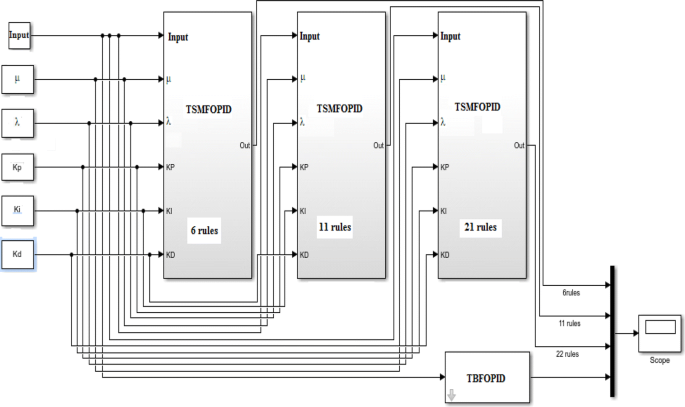

  

  TSMFOPID controller with 6, 11 and 21 memberships

• 2. Realize the TS fuzzy formula for the fractional orders of integral and derivative parameters (λ and μ) as shown in Fig. 8. If the input is λ, the block diagram represents TSMFOI, while if the input is μ, the block diagram represents TSMFOD.

  Fig. 8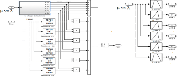

  

  Block diagram of the fractional orders of the integral and derivative

• 3. Implement the final outputs of the fuzzy systems that inferred for the TSMFOD or TSMFOI using the following equation [12]:

  $$ {\text{Out}}_{I} = \frac{{\mathop \sum \nolimits_{{\lambda_{i} }} W_{{\lambda_{i} }} \cdot F_{{\lambda_{i} }} }}{{\mathop \sum \nolimits_{{\lambda_{i} }} W_{{\lambda_{i} }} }} ;\;{\text{out}}_{D} = \frac{{\mathop \sum \nolimits_{{\mu_{i} }} W_{{\mu_{i} }} \cdot F_{{\mu_{i} }} }}{{\mathop \sum \nolimits_{{\mu_{i} }} W_{{\mu_{i} }} }} ; $$

  (4)

  where λ_i, µ_iϵ {0.0, 0.2,0.4,0.6,0.8,1.0}; for 6 rules, λ_i, µ_i ϵ {0, 0.2, 0.4, 0.6, 0.8, 1, 1.2, 1.4, 1.6, 1.8, 2}; for 11 rules, λ_i, µ_i ϵ {0, 0.1, 0.2, 0.3, 0.4, 0.5, 0.6, 0.7, 0.8, 0.9, 1, 1.1, 1.2, 1.3,1.4, 1.5, 1.6, 1.7, 1.8, 1.9, 2} for 21 rules, W_λi is the weight of λ_i, W_µi is the weight of µ_i, F_λi is the output of TBFOPI whose λ value is λ_i and F_µi is the output of TBFOPD whose µ value is µ_i [12].

Based on the pervious different cases for simulation results are implemented performed using the MATLAB toolbox.

Case 1: Comparison between fractional integral Iλ for TSMFOPID and TBFOPID controllers

Comparison between fractional orders of integral Iλ for TSMFOPI and TBFOPI controllers can be made using 6, 11 and 21 rules. The simulation results are obtained using the MATLAB toolbox. In [12], the simulation time for comparison was 10 s. In this paper, the simulated time is equal to 100 s. The step dynamic response at λ = 0.98, µ = 0.0, k_p = 0.0, k_d = 0.0 and k_i = 8.16 is shown in Fig. 9. It is noted that using six rules, TSMFOI shows large difference value than TBFOI. However, using 11 rules gives nearest response of the TBFOI, while using 21 rules gives approximately similar to the TBFOI.

Fig. 9

Step dynamic response of TSMFOI and TBFOI

Case 2: Comparison between fractional derivative Dμ for TSMFOPID and TBFOPID controllers

The same simulation is repeated for comparison between fractional orders of derivative Dμ for TSMFOPD and TBFOPD controllers using 6, 11 and 21 rules. The ramp dynamic response at λ = 0.0, µ = 0.98, k_p = 0.0, k_d = 2.0 and k_i = 0.0 is shown in Fig. 10. Similar results are obtained and verified that 21 rules should be preferred for TS fuzzy design for TSMFOD.

Fig. 10

Ramp dynamic response of TSMFOD and TBFOPD

Case 3: Comparison between TSMFOPID and TBFOPID controllers

In this case, the simulation is started by calculating the optimal values of the unknown five parameters (k_p, k_d, k_i, λ and μ) of FOPID controller for the (LFC) considered application. Ant optimization (that has full details in [17]) algorithm is performed through selected cost function given by Eq. (5).

$$ J = \frac{1}{{[C_{1} (t_{r} - t_{rd} ) + c_{2} (M_{P} - M_{pd} ) + c_{3} (t_{s} - t_{sd} ) + C_{4} (e_{ss} - e_{ssd} )]}} $$

(5)

subject to the boundary conditions (constraints):

$$ \begin{aligned} {\text{k}}_{{{\text{j}}_{{\rm min} }}} & \le {\text{k}}_{j} \le {\text{k}}_{{{\text{j}}_{{\rm max} }}} \left( {{\text{j}} = {\text{P}}\;{\text{or}}\;{\text{D}}\;{\text{or}}\;{\text{I}}} \right) \\ & 0 < \lambda_{{\rm min} } \le \lambda \le \lambda_{{\rm max} } \\ & 0 < \mu_{{\rm min} } \le \mu \le \mu_{{\rm max} } \\ \end{aligned} $$

where C1, C2, C3, and C4 are arbitrary (weight) values and in the considered case C1 = C2 = C3 = C4 = 1. The trd, essd and Mpd represent the desired of each rise time, steady-state error and over shoot, respectively. In this case, trd, essd and Mpd are equal to zero. The obtained results of the TBFOPID using Ninteger toolbox are kp = 4.567, kd = 1.962, μ = 0.922, ki = 8.159 and λ = 0.998. Figures 11 and 12 show the results corresponding to simulations of the considered application LFC driven by TBFOPID and TSMFOPID when the controlled system is subjected to step disturbance ∆Pd = 0.05 p.u. The TSMFOPID is designed using TS fuzzy technique with 6, 11 and 21 rules. It is deduced that the TSMFOPID designed by 21 rules is almost the same behavior of TBFOPID. Also, it s easily proven the same results for the control output.

Fig. 11

Dynamic responses of ∆F controlled by TBFOPID and TSMFOPID

Fig. 12

Dynamic responses of control output controlled by TBFOPID and TSMFOPID

Case 4: Effect of μ for Dμ and λ for Iλ on TBFOPID controller

Figure 13 shows the ∆F responses when the controlled system is driven with varying values of 0 < λ > 2 while μ < 1 and kept constant. The ∆Pd is 0.05 p.u (step input). From these results, it can be deduced that the value of λ effect on the system performance significantly and in some application λ may be taken 0 < λ > 2. Figure 14 shows the simulation results when the controlled system is subjected to the same disturbance and λ < 1 (kept constant) and 0 < μ > 2. It can be noted that μ adds flexibility and makes the system more enhancing its dynamic performances compared to derivative PID. Also, μ may be taken values in some applications 0 < μ > 2.

Fig. 13

Dynamic responses of ∆F controlled by TBFOPID and λ > 1

Fig. 14

Dynamic responses of ∆F controlled by TBFOPID and μ > 1

Observations From the above simulation plots, it can be observed that TS fuzzy design for FOPID model should be taken 21 rules. The fractional orders of integral and derivative values may have (λ and μ) 0 < μ > 2 and 0 < λ > 2, and each one of these values has significantly affect the responses of the controlled system with FOPID.

The second category is concerned with interval type-2 fuzzy self-tuning.

Type-2 fuzzy logic systems and interval type-2 fuzzy sets

Type-2 fuzzy logic system is proposed as an extension of T1FLSs. While designing T1FLSs, expertise and knowledge are needed to decide both the MFs and fuzzy rules. The T1FLSs, whose MFs are type-1 fuzzy sets, are unable to directly handle rule uncertainties [6, 7]. To deal with this problem, the concept of type-2 fuzzy sets was introduced by Zadeh as an extension of T1FLSs with the intention of being able to model the uncertainties that invariably exist in the rule base of the system [6, 7]. The upper membership function (UMF) and lower membership function (LMF) of $\tilde{A}$ are two T1 membership functions that bound the footprint of uncertainty (FOU) as shown in Fig. 15. The UMF of $\tilde{A}$ is the upper bound of the FOU $\left( {\tilde{A}} \right)$ and denoted as $\bar{\mu }_{{\tilde{x}}} \left( x \right)\forall x \in X$, and the LMF is the lower bound of the FOU $\left( {\tilde{A}} \right)$ and denoted as $\underset{\raise0.3em\hbox{$\smash{\scriptscriptstyle-}$}}{\mu }_{{\tilde{x}}} \left( x \right)\forall x \in X$. The UMF and LMF can be characterized as follows [9]:

$$ \bar{\mu }_{{\tilde{x}}} \left( x \right) = \overline{{FOU\left( {\tilde{A}} \right)}} \forall x \in X $$

(6)

$$ \underset{\raise0.3em\hbox{$\smash{\scriptscriptstyle-}$}}{\mu }_{{\tilde{x}}} \left( x \right) = \underline{{FOU\left( {\tilde{A}} \right)}} \forall x \in X $$

(7)

The computations of fuzzification and inference for IT2-FLC were given and discussed in [9]. For this operation, type reduction to convert IT2-FLC into a T1-FLC is performed [6,7,8,9]. There are several methods of type reduction. In this paper, the “center-of-sets” type reduction is used. The calculations of this method were done and given in [8]. In addition, the defuzzification method is determined to convert type-reduced set into crisp output of an IT2-FLS [9].

Fig. 15

FOU, UMF and LMF for an IT2 FS Ã

Online interval type-2 fuzzy self-tuning for the TSMFOPID controller

To update the TSMFOPID controller at different operating points using IT2-FLS, three types of tuning are implemented.

• The first type tunes the proportional, integral and derivative gains (kp, kd and ki).

• The second type tunes the fractional orders of integral and derivative gains (λ and μ).

• The third type modifies the five parameters of FOPID controller (kp, kd, ki, λ and μ).

Figure 16 shows the block diagram of an IT2-FS technique as trainer for considered application. This diagram can be used for the three types of tuning. For each type, the terminal of the untuning can be became constant for its optimal value. For the system under study, the universe discourse for both e(t) and Δe(t) for k_p2, k_i2, k_d2, μ and λ has normalized with [0,5], [0,5], [0,5], [0,5], [0,5], [0,2] and [0,2], respectively. The linguistic labels are {Negative Big, Negative Medium, Negative Small, Zero, Positive Small, Positive Medium, Positive Big}, and the linguistic labels of the outputs are {Zero, Medium Small, Small, Medium, Big, Medium Big, Very Big}. The IT2 of membership function for e(t) and Δe(t) is shown in Fig. 17, while that of the output for k_p, k_i and k_d is shown in Fig. 18. The membership functions for μ and λ are similar and plotted in Fig. 19.

Fig. 16

Type-2 fuzzy self-tuning propose

Fig. 17

Membership function of inputs e and Δe

Fig. 18

Membership function for K_P, K_I and K_D

Fig. 19

Membership function for μ and λ

The control rules used for T1FST of TSMFOPID controller for determining the output gains from fuzzy controller were given [4,5,6,7]. This general equation of the FOPID can be written as:

$$ u\left( s \right) = \left( {k_{p} + \frac{{k_{i} }}{{s^{\lambda } }} + k_{d} \cdot s^{\mu } } \right)e\left( s \right) $$

(8)

This equation of the TSMFOPID after fuzzy effect can be written as:

$$ u\left( s \right) = \left( {k_{p} *k_{pt} + \frac{{k_{i} *k_{i} t}}{{s^{\lambda *\lambda t} }} + k_{d} \cdot k_{dt} s^{\mu *\mu t} } \right)e\left( s \right) $$

(9)

where $k_{p3} = k_{p} *k_{pt} , k_{i3} = k_{p} *k_{pt} ,k_{d3} = k_{d} \cdot k_{dt} ,\lambda = \lambda *\lambda t,\mu = \mu *\mu t$; k_p3, k_i3, k_d3 are the output gains from fuzzy controller of IT2FST; Kei: error input normalizing gain, i = 1,2,3; and K∆ei: ∆error input normalizing gain, i = 1,2,3.

The IT2-FS tuner of the TSMFOPID controller shown in Fig. 16 is designed and simulated for LFC single area with different three types of tuning. Contrary to the trial-and-error selection and to avoid large simulation efforts for choosing IT2-FS tuner normalizing gains, this problem is formulated as an optimal problem. The previous cost function given in Eq. (5) and ant colony optimization based on lower and upper values of each unknown normalizing gains are used. The values of these gains for the three types of IT2-FS tuner are given in Table 1.

Table 1 Optimal values for normalizing gains of the three tuning cases

To demonstrate the effectiveness of IT2FST by three types on the TSMFOPID controller, several cases are carried out and the results are presented and compared with those of the T1FST.

• Case 1 IT2-FS tunes the kp, ki and kd for TSMFOPID.

• Case 2 IT2-FS tunes the λ and μ for TSMFOPID.

• Case 3 IT2-FS tunes the k_P, k_i, k_d, λ and μ for TSMFOPID.

After TSMFOPID was implemented, the controller is combining with the IT2-FS technique to compose the online fuzzy self-tuning controller. The three cases of tuning are implemented for LFC to test the validity of these cases of tuning. For different types of the tuning, the simulation is started when the LFC is being subjected to a step load change of 0.5% inΔPd. For case 1, Figs. 20 and 21 show the response of ΔF and its respective response with tuning only k_P, k_i and k_d . The response of the controller output is given in Fig. 21. It is obvious that self-tuning gives improvement performance in both transient and the steady-state response. IT2-FS tuning with TSMFOPID has less overshoot and has a smaller steady-state error compared to the TSMFOPID controller. For case 2, Figs. 22 and 23 show the dynamic responses after tuning using λ and μ, while k_P, k_i and k_d are kept constant. It is observed that the tuning responses have small better performance with respect to TSMFOPID. In case 3, IT2-FS for TSMFOPID is tuned using k_P, k_i, k_d, λ and μ. Figures 24 and 25 show the responses for this case. It is observed that the proposed tuning of IT2-FS for TSMFOPID gives better response with fewest oscillations and fast reaching to the zero-steady-state value. Also, the response of controller output is given in Fig. 25. It can be observed that the damping of oscillation is much improved for the transient error in both ΔF and controller output.

Fig. 20

Response of ΔF via IT2FST (k_P, k_i and k_d)

Fig. 21

Controller output via IT2FST (k_P, k_i and k_d)

Fig. 22

Response of ΔF via IT2FST (λ and μ)

Fig. 23

Controller output via IT2FST (λ and μ)

Fig. 24

Response of ΔF via IT2FST (k_p, k_i, k_d, λ and μ)

Fig. 25

Controller output via IT2FST (k_p, k_i, k_d, λ and μ)

Case 4: Comparison between cases 1–3

In Figs. 26 and 27, a comparison between cases 1–3 is made. It is observed that the proposed case 3 gives better response with fewest oscillations and fast reaching to the zero-steady-state value than the other cases. The simulation results have shown that the tuning using k_P, k_i, k_d, λ and μλ and μ are capable of providing sufficient damping to system oscillations and improving the dynamic performance of the application.

Fig. 26

Response of ΔF via IT2FST (k_p, k_i, k_d, λ and μ)

Fig. 27

Controller output via IT2FST (k_p, k_i, k_d, λ and μ)

Case 5: Comparison between IT2FST and T1FST for TSMFOPID

In order to compare the IT2FST and T1FST for TSMFOPID, a disturbance of 5% is applied in ΔPd. As shown in Fig. 28, the IT2FST is found to be most efficient in improving the steady-state and transient responses with effect of the disturbance. A significant improvement in the system performance is obtained with the proposed IT2FST than T1FST for the controller output as shown in Fig. 29.

Fig. 28

Response of ΔF via IT2FST and T1FST for TSMFOPID (k_p, k_i, k_d, λ and μ)

Fig. 29

Controller output via IT2FST and T1FST for TSMFOPID (k_p, k_i, k_d, λ and μ)

Case 6: Comparison between IT2FST and T1FST for TSMFOPID under parameter uncertainties

To show the validity of the proposed IT2FST for TSMFOPID under the effect of the parameter uncertainties, the comparison between IT2FST and T1FST for TSMFOPID is made. The details for self-tuning for T1FST were mentioned in [4,5,6,7]. The normalizing gains for T1FST are optimally calculated using ant colony optimization and the same cost to make the comparison fair. The rule base for determining k_P1, k_i1, k_d1, λ and μ was given in [4,5,6]. For the LFC block diagram, a nominal value of Tt is maintained constant for 0 ≤ t ≥ 2, 50% of Tt is decreased for 2 ≤ t ≥ 4, 60% of Tt is increased from nominal value for 4 ≤ t ≥ 6 and it is maintained constant for 6 ≤ t ≥ 10%. The system uncertainty parameters are applied to each of IT2FST and T1FST for TSMFOPID controllers when the step disturbance of 5% is applied in ΔPd. From Figs. 30 and 31, it is clear that the system equipped with IT2FST shows better performance than T1FST from overshoot, oscillations and settling time point of view. Moreover, in Fig. 31, the superiority of the IT2FST over the T1FST is clearly seen, whereas the T1FST completely has overshoots at last and then reaches steady-state value.

Fig. 30

Response of ΔF via IT2FST and T1FST for TSMFOPID (k_p, k_i, k_d, λ and μ) with parameter uncertainties

Fig. 31

Controller output response via IT2FST and T1FST for TSMFOPID (k_p, k_i, k_d, λ and μ) with parameter uncertainties

Conclusion

IT2FST and TSMFOPID controllers are combined to design a new fuzzy self-tuning tool to compensate the undesired effects of parameter uncertainties and absorb the sudden change of the disturbances. TS is used to construct the modified FOPID with external five terminals. This is to overcome the technical constraint of TBFOPID Simulink block that does not allow changing the controller parameters during the online fuzzy self-tuning simulation time. TS fuzzy is designed in a general form by 11 and 21 memberships with λ and μ being greater than 0 and less than 2, and this is essential in control processes. The best representation for the TSMFOPID is obtained when the TS technique is designed by 21 or 11 memberships, respectively. Three types of IT2FST for TSMFOPID are implemented. IT2FST can suppress the system uncertainty in a small time compared to T1FST. The proposed approaches are implemented for single-area load frequency control as a case study. From the simulation results, it was found that the best performance is achieved when all of the five parameters of the controller are to be tuned. Finally, it can be concluded that the proposed IT2FST for TSMFOPID controller improves the performance characteristics and provides flexibility as compared to TSMFOPID with T1FST.

References

Silva GJ, Datta A et al (2002) New results on the synthesis of PID controllers. IEEE Trans Autom Control 47(2):241–252
Åström K, Hägglund T (2006) Advanced PID control. The Instrumentation, Systems, and Automation Society (ISA), Research Triangle Park
Algreer MM, Kuraz YRM (2008) Design fuzzy self tuning of PID controller for chopper-fed DC motor drive. Al-Rafidain Eng J 16(2):54–66
Abdel Ghany MA, Bahgat ME, Refaey WM, Hassan FN (2017) Design of fuzzy self tuning PID load frequency controller for the Egyptian power system. J Al-Azhar Univ Eng Sect 12(42):77–89
El-Samahy AA, Shamseldin MA (2016) Brushless DC motor tracking control using self-tuning fuzzy PID control and model reference adaptive control. Ain Shams Eng J 9(3):341–352
Mendel JM, John RIB (2002) Type-2 fuzzy sets made simple. IEEE Trans Fuzzy Syst 10(2):117–127
Mende JM, John RI, Liu F (2006) Interval Type-2 fuzzy logic systems made simple. IEEE Trans Fuzzy Syst 14(6):808–821
Mendel JM, John RIB (2002) Footprint of uncertainty and its importance to Type-2 fuzzy sets. In: Proceedings of the 6th IASTED international conference on artificial intelligence and soft computing, Banff, Canada, pp 587–592
Mendel JM (2007) Type-2 fuzzy sets and systems: an overview. IEEE Comput Intell Mag 21:20–29
Bensenouci A, Shehata M (2015) Optimized FOPID control of a single link flexible manipulator (SLFM) using genetic algorithm. Appl Mech Mater 704:336–340
Shamseldin MA, EL-Samahy AA, Ghany AMA (2016) Different techniques of self-tuning FOPID control for Brushless DC motor. In: 2016 eighteenth international middle east power systems conference (MEPCON), Cairo, pp 342–347
Gaballa MS, Bahgat M, Abdel Ghany AM (2017) A novel technique for online self-tuning of fractional order PID, based on Takaji–Sugeno fuzzy. In: Nineteenth international middle east power systems conference (MEPCON), Menoufia University, Egypt, 19–21 December 2017
Bensenouci A, Abdel Ghany AM (2010) Performance analysis and comparative study of LMI-based iterative PID load-frequency controllers of a single-area power system. WSEAS Power Syst J 5(2):85–97
Serra GLO, Ferreira CCT (2009) Takagi–Sugeno fuzzy control method for nonlinear systems. In: 2009 IEEE international symposium on computational intelligence in robotics and automation–(CIRA), Daejeon, pp 492–496
Wong LK, Leung FHF, Tam PKS (2002) Design of fuzzy logic controllers for Takagi–Sugeno fuzzy model based system with guaranteed performance. Int J Approx Reason 30(1):41–55
Gaballa MS, Bahgat M, Abdel Ghany AM (2017) Practical implementation of TS-fuzzy PID to control a dual-axis sun tracker of a photo-voltaic panel. In: Nineteenth international middle east power systems conference (MEPCON), Menoufia University, Egypt, 19–21 December 2017
Abdel Ghany MA, Bahgat ME, Refaey WM, Hassan FN (2014) Ant colony optimum tuning of PID load frequency controller for the Egyptian power system. In: Sixteenth international middle east power systems conference (MEPCON’14), Ain Shams University, Egypt, 2014
Acknowledgements
I would like to express my deepest appreciation to all those who provided me the possibility to complete this research.
Funding
Research support from author’s affiliations.
Author information
Authors and Affiliations
Contributions
MAAG was involved in design and control implementation. MEB reviewed the simulation results. WMR and SS reviewed the paper. All authors read and approved the final manuscript.
Corresponding author
Ethics declarations
Competing interests
The authors declare that they have no competing interests.
Additional information
Publisher's Note
Springer Nature remains neutral with regard to jurisdictional claims in published maps and institutional affiliations.
Rights and permissions
Open Access This article is licensed under a Creative Commons Attribution 4.0 International License, which permits use, sharing, adaptation, distribution and reproduction in any medium or format, as long as you give appropriate credit to the original author(s) and the source, provide a link to the Creative Commons licence, and indicate if changes were made. The images or other third party material in this article are included in the article's Creative Commons licence, unless indicated otherwise in a credit line to the material. If material is not included in the article's Creative Commons licence and your intended use is not permitted by statutory regulation or exceeds the permitted use, you will need to obtain permission directly from the copyright holder. To view a copy of this licence, visit http://creativecommons.org/licenses/by/4.0/.
About this article
Cite this article
Ghany, M.A.A., Bahgat, M.E., Refaey, W.M. et al. Type-2 fuzzy self-tuning of modified fractional-order PID based on Takagi–Sugeno method. Journal of Electrical Systems and Inf Technol 7, 2 (2020). https://doi.org/10.1186/s43067-019-0009-9
Received:
Accepted:
Published:
DOI: https://doi.org/10.1186/s43067-019-0009-9