Risk mitigation in electric power systems: Where to start?

Abstract

Power grids are becoming increasingly intelligent. In this regard, they benefit considerably from the information technology (IT) networks coupled with their underlying operational technology (OT) networks. While IT networks provide sufficient controllability and observability of power grid assets such as voltage and reactive power controllers, distributed energy resources, among others, they make those critical assets vulnerable to cyber threats and risks. In such systems, however, several technical and economic factors can significantly affect the patching and upgrading decisions of their components including, but not limited to, limited time and budget as well as legal constraints. Thus, resolving all vulnerabilities at once could seem like an insuperable hurdle. To figure out where to start, an involved decision maker (e.g. a security team) has to prudently prioritize the possible vulnerability remediation actions. The key objective of prioritization is to efficiently reduce the inherent security risk to which the system in question is exposed. Due to the critical role of power systems, their decision makers tend to enhance the system resilience against extreme events. Thus, they seek to avoid decision options associated with likely severe risks. Practically, this risk attitude guides the decision-making process in such critical organizations and hence the sought-after prioritization as well.Therefore, the contribution of this work is to provide an integrated risk-based decision-support methodology for prioritizing possible remediation activities. It leverages the Time-To-Compromise security metric to quantitatively assess the risk of compromise. The developed risk estimator considers several factors including: i) the inherent assessment uncertainty, ii) interdependencies between the network components, iii) different adversary skill levels, and iv) public vulnerability and exploit information. Additionally, our methodology employs game theory principles to support the strategic decision-making process by constructing a chain of security games. Technically, the remediation actions are prioritized through successively playing a set of dependent zero-sum games. The underlying game-theoretical model considers carefully the stochastic nature of risk assessments and the specific risk attitude of the decision makers involved in the patch management process across electric power organizations.

Introduction

On 12 May 2017, a very disruptive malware called WannaCry was observed. WannaCry infected about 250,000 computers in 150 countries, particularly in critical systems. It resulted in huge damage costs predicted about 4 billions of dollars (Berr 2017). Interestingly, WannaCry exploited a known and well-documented Windows-specific vulnerability (NVD 2017). On top of this, Microsoft released a vulnerability patch on 14 March 2017 towards fixing this vulnerability and providing protection against any potential attacks. That is, the infected systems would not have been subject to this attack, had these systems been updated during the two-month period before the attack. This raises the question, why had these (critical) systems not been patched timely?

To answer this question, we reviewed some security standards and guidelines, including (BSI: Bundesamt für Sicherheit in der Informationstechnik 2018; Mell et al. 2005; Souppaya and Scarfone 2013). Based on our review, the key reasons for this phenomenon are: i) strict patch validation process, ii) limited available security resources, and iii) high reliability and availability requirements. Broadly speaking, while standards encourage, if not oblige, organizations to perform maintenance and update of their assets in a timely manner, they impose a very rigorous and time-consuming patch testing procedures before deployment. However, available security resources are usually scarce and expensive. Such constraints would prevent organizations from fully resolving all of the vulnerabilities that their assets are at risk from. Moreover, power grids require high reliability/availability of their components, only allowing for short periods of downtime (IEC61508 2010). Thus, any maintenance and upgrade decisions have to be made very prudently, taking such requirements into consideration. It is, therefore, very difficult – if not impossible – to have an operational system that is completely vulnerability-free. Another complicating factor is the rapidly growing volume of released patches. This can overburden security teams, hence the reason for a poor patch management process. All these issues make the question (where to start implementing remediation actions?) pivotal in patch management processes.

A proper patch prioritization represents an efficient way of dealing with the aspects of security economics and risk management. It seeks to maximize the benefits of the available resources through focusing on the most critical issues first and hence minimize the inherent security risk in an effective manner (Giani et al. 2012; Gonzalez-Granadillo et al. 2015). Such a process would certainly involve i) the use of some comparative judgments to define a ranking system, and ii) a decision-support technique to evaluate and compare the different options of a prioritization decision. In this context, the vast majority of existing prioritization practices depends on merely qualitative measures and/or severity-based decision-making processes. Qualitative judgments and measures are typically highly subjective. Thus, they might lead to improper decisions heavily biased by individual perspectives. Such decisions could be influenced by an inaccurate interpretation of a system state caused by a forced consensus of the judgments as well as disregard of diversity. The second limitation is that existing prioritization approaches are vulnerability-centric; that is, their decisions always dictate that the vulnerability with the highest severity score should be resolved first. However, such decisions are not necessarily the best response in terms of minimizing risk. Suppose all devices in a network are affected by the same severe vulnerability like CVE-2017-0144 with the severity rating of 8.1 HIGH (CVSS v3.0) (NVD 2017). In this case, all devices – regardless of their characteristics or location on the network – are at high risk of being compromised and have the same priority to be patched first. Such decisions are, however, not always actionable, thereby extremely confusing an involved security team.

In practice, the process of risk management and assessment involves several other technical and organizational factors, not only the severity scores. Hence, vulnerability prioritization that is naturally severity-based is not a robust option for patch prioritization that is risk-based. A recent Gartner research report stresses the need for a risk-based prioritization approach that can correlate several factors such as asset values, severity of vulnerabilities, public exploit information, and attacker characteristics (Bhajanka and Lawson 2018). This implies that the sought-after prioritization should incorporate the decision-making process with proper risk assessment techniques. Throughout this work, the Time-To-Compromise (TTC) metric is pursued as a comparative security metric to analyze and quantify the risk mitigation impact of possible security actions. Typically, TTC metric is used to deliver single-point estimates such as Mean-Time-To-Compromise (MTTC) (Leversage and Byres 2008). However, these estimates cannot robustly deliver an accurate risk prediction due to different uncertainties involved in real systems and underlying observational data. Therefore, we present a generalized stochastic TTC model integrated with Monte Carlo simulation¹ techniques to account for the input data variability and inherent prediction uncertainty.

Like the vast majority of security decisions, prioritization decisions are made in a non-cooperative environment, in which two competitors, an involved decision maker (hereafter called the defender) and a potential attacker, seek to maximize their own benefits, each from a certain space of possible actions or strategies. To address this fact, our methodology leverages game theory principles to model the strategic behaviour of the involved players and to advise the defender on the best response to potential compromise plans. Generally, remote attackers seek to exploit cyber vulnerabilities present in IT networks to obtain unauthorized access to interconnected OT networks, thereby causing significant damages. Due to their crucial role in our modern society, extreme (failure) events in power grids can be associated with irreversible consequences to the public health, safety, and security. Thus, the defender of such systems tends to boost the system resilience through avoiding situations in which high-level risks are more likely to happen. In a recent study on the power system resilience, Bie et al. stress the vital importance of being able to mitigate (high-level) extreme risks as a condition for having resilient electricity infrastructures (Bie et al. 2017). To the best of our knowledge, this specific risk attitude imposed by the criticality of electric power systems is not well-addressed in existing prioritization approaches. Therefore, the presented game-theoretical model accounts for the aforementioned risk attitude by relying on a stochastic (tail) order reflecting the desired preference relation between the uncertain risk assessments. It is worth mentioning that traditional game-theoretical models, in which an expected utility (loss) optimization paradigm (Von Neumann and Morgenstern 2007) is overwhelmingly pursued, are not compatible with the comprehensive nature of our risk assessments. Traditional models rely on scalar-valued payoffs, while our TTC-based risk assessments are distribution-valued.

As we will see later in this work, the novelty of our approach lies in the way it integrates the risk attitude of the decision makers involved in the patch management operations across electric power organizations into the prioritization process. The rest of this paper is structured as follows: “Related work” section outlines the existing TTC models and their limitations as well as some related game-theoretical patch management approaches. Further, it includes a detailed overview of our contribution. The improved stochastic TTC model and the involved game-theoretical model are formally described in “Stochastic TTC model” section and “Security game model” section, respectively. Our decision-support methodology is explained in “Decision-support methodology” section, as well as applied in “Use Case” section and comprehensively evaluated in “Evaluation of the prioritization options” section. Finally, concluding thoughts and future research directions follow in “Conclusion” section.

Related work

Electric power systems are cyber-physical systems whose operations and processes are orchestrated, controlled, and monitored using computer networks. Despite their tremendous benefits, computer networks make critical components of electric power systems at risk of cyber threats. Therefore, mitigation of cyber risks in electric power networks has attracted a lot of research attention. Among recent research activities on enhancing cyber security of power systems, Shelar et al. proposes a game-theoretical model to optimize the security strategy of electricity distribution networks (Shelar and Amin 2016). They consider a specific adversary model, in which false data injection attacks are used to compromise vulnerable distributed energy resource (DER) nodes. In Ciapessoni et al. (2016), the authors propose an in-depth security analysis of electric power systems. Their approach relies on an extended definition of risk, which includes factors such as threats, vulnerability, contingency, and impact. It defines a dynamic selection of contingencies based on the current identified threats.

Besides security enhancement methodologies, security metrics such as TTC have attracted significant attention from the research community as a means to assess and prioritize various security risks as well as defense strategies. Among the earliest works of modeling and applying TTC metric are McQueen et al. (2006a); McQueen et al. (2006b); Leversage and Byres (2008). In McQueen et al. (2006a); McQueen et al. (2006b), the authors propose a basic model for estimating the time to compromise a specific control system. The model is leveraged to calculate the shortest path (in terms of its time) to reach and damage a target node of a system of interest. This model has been originally designed to provide estimates of the risk associated with potential attacks against critical elements of electric power systems, which are SCADA control systems. In Leversage and Byres (2008), the authors employ the same TTC model to estimate MTTC values of different systems and mitigation strategies used to enhance security of SCADA systems. More recent research work such as Nzoukou et al. (2013); Zhang et al. (2015) proposes new models for estimating MTTC values of different security solutions and configurations applied in critical infrastructure environments such as electric power systems. They involve the use of vulnerability-based attack graphs. Each vulnerability represents a state in the final graphical model and has its own MTTC value. Ultimately, the final MTTC estimate is computed based on the MTTC values of the states and their CVSS²-driven probabilities. In Zhang et al. (2015), the MTTC metric is modified to evaluate the reliability of power systems using the IEEE RTS79 as a test system. The presented results show that the power system becomes less reliable with the increased rate of successful attacks on the cyber components. The main limitations of existing TTC models are threefold. Firstly, these models yield merely single-point TTC estimates. Such estimates do not account for the uncertainty, ambiguity, and variability of involved observational data. Further, they can convey misleading indications of extreme risks due to aggregation. Thus, they can not ensure robust and accurate risk measures. Secondly, the models shown in (McQueen et al. 2006a; 2006b) do not address explicitly the characteristics of potential zero-day vulnerabilities. Thirdly, the models in Nzoukou et al. (2013); Zhang et al. (2015) use vulnerability-based attack graphs, which suffer from the state explosion problem, where the size of the state space becomes quickly unmanageable. This can significantly limit the applicability of the models in real-world scenarios.

Game theory, in its turn, is widely used in the context of strategic security planning. With regard to vulnerability patch management, the authors in Gianini et al. (2015); Maghrabi et al. (2017) combine game theory principles and vulnerability scoring techniques to prioritize vulnerabilities based on assessed severity indicators. As discussed in “Introduction” section, vulnerability prioritization that is naturally severity-based is not adequate for patch prioritization processes, which seek to reduce the risk of compromise in an efficient way. In Panaousis et al. (2014), the authors discuss applying game theory to advise security managers on how to optimally invest in security controls. Their game-theoretical model assumes deterministic assessments (scalar-valued payoffs), and hence does not account for inherent prediction uncertainties. Beyond that, the prioritization decisions made by existing game-theoretical frameworks do not consider the aforementioned risk attitude of the decision makers involved in the protection of electric power systems. In traditional game models, extreme risks may still be undesirably probable though the average risk has been optimized.

Our Contribution: This paper provides a decision-support methodology that assists the defender of an electric power system in prioritizing the possible vulnerability patch actions according to their risk mitigation impact. Strictly speaking, the respective actions are successively prioritized with the aid of a chain of security zero-sum games. The chain depends on a general game-theoretical model with distribution-valued payoffs to account for the process of decision-making under uncertainties. The game model benefits from a stochastic (tail) order to incorporate the risk attitude, imposed by the criticality of the investigated electric power systems, into the decision-making process. The security (compromise) risk is quantified using a developed TTC estimator that has the following features: i) simple and easy to understand, even for non-professionals; ii) practical through the use of asset-centric compromise graphs instead of vulnerability-centric attack graphs; and iii) addressing the inherent uncertainty and variability of involved observational/statistical data using Monte Carlo simulation techniques. Therefore, the obtained TTC-based risk estimates are comprehensive, thereby conveying rich information on the two primary dimensions of risk descriptors, i.e. risk impact levels and their occurrence probabilities. The developed risk estimator can be leveraged to give indications on a system robustness against not only technical vulnerabilities but also social and organizational factors. However, for the sake of simplicity, we limit the underlying TTC model presented in this paper to only software (technical) vulnerabilities. Due to the absence of reliable information about the preferences of potential adversaries, we assume there is a completely negative correlation between the two players of our games. This yields that the game model is zero-sum, thereby enabling the defender to defend the network against the worst-case compromise scenario.

Stochastic TTC model

A TTC estimate denotes to a prediction of the time needed for a potential adversary to exploit technical vulnerabilities of a system towards gaining an unauthorized access to it. This corresponds to the time of a graph transition connecting a pair of nodes (SOuRCe, DESTination) given that the adversary controls the SORC node and seeks to compromise the DEST through exploiting its vulnerabilities. To estimate a Transition-Time-To-Compromise (TTTC), we developed a stochastic model that takes into account a set of inputs summarized in Table 1. The inputs depend on existing statistical observations and outcomes of a security analysis of the network in question. Our TTC model delivers comprehensive TTC estimates described using probability distributions instead of single-point estimates delivered by the basic model presented in McQueen et al. (2006b).

Table 1 A list of our TTC model inputs

Basically, our model rests on the following two probabilities:

• p₀: the probability that an adversary find “zero” fully functioning exploit (from his/her M available exploits) for the n vulnerabilities visible at DEST, given that there are totally N known vulnerabilities. Based on the definition of the hypergeometric distribution³ :

  $$ p_{0} =\frac{{N-M \choose n}}{{N \choose n}} $$

  (1)

• $\hat {p}$: the probability that an adversary fails to craft any functioning exploit for the known vulnerabilities visible at DEST. $\hat {p}$ depends mainly on S (0≤S≤1≡Expert) and (n_L,n_H) (see Table 1). More precisely, if DEST has no known vulnerability then $\hat {p}$ should be 1. But, $\hat {p}$ should be very small if the adversary has in-depth knowledge (i.e. S≈1) and DEST has a known low-complex vulnerability; it can be approximated by $\hat {p} = 1-S$. Under the assumption of independent vulnerabilities, $\hat {p}$ can be generalized as follows:

  $$ \hat{p} = (1-S+\hat{l})^{n_{L}}\times(1-S+\hat{h})^{n_{H}} $$

  (2)

  where $\hat {l}$ and $\hat {h}$ are two control parameters⁴ reflecting that an adversary’s chance of failing is higher against high-complex vulnerabilities rather than low-complex ones.

In our model, an adversary trying to compromise a node DEST can be in one of three random processes. For each process i, we are interested in two quantities; namely

• p_i: the probability of being in process i, and

• t_i: the time needed for a successful compromise attempt given that the adversary is in process i.

Process 1: An adversary has identified one or more known vulnerabilities and has one or more exploits readily available. Therefore, the probability that the adversary is in Process 1 is the complement of the probability that an adversary has zero exploit readily available, which is p₀ as defined in Eq. (1). This yields:

$$p_{1} = 1-p_{0} = 1 - \frac{{N-M \choose n}}{{N \choose n}} $$

The time needed for an adversary in Process 1 can be described using the random variable β₁ as described in Table 1. Typically, the time and the adversary skill level vary inversely. Thus, we modify the time estimate in such a way that the time increases if the adversary skill level decreases. This yields:

$$t_{1} = \beta_{1} \times \frac{1}{S} $$

Process 2: An adversary has identified one or more known vulnerabilities but couldn’t find a functioning exploit readily available and s/he tries to craft an own exploit. p₂ is defined as the product of the probability of having zero readily available exploit (p₀) and the probability of successfully developing at least one functioning exploit for at least one of the n visible vulnerabilities; i.e. $1-\hat {p}$. This yields:

$$p_{2} = p_{0} \times (1-\hat{p}) = \frac{{N-M \choose n}}{{N \choose n}} \times (1-(1-S+\hat{l})^{n_{L}}\times(1-S+\hat{h})^{n_{H}}) $$

Then, t₂ depends on i) the time needed to craft a working exploit modeled as a random variable Γ_5.8 in Table 1, and ii) the expected number of tries ET until the adversary can develop a fully working exploit code for one of the n vulnerabilities.

$$ ET = S \times (1 + \sum_{i=2}^{n-C+1}[ i \times \prod_{j=2}^{i} (\frac{n-C-j+2}{n-j+1})]) $$

(3)

This yields:

$$t_{2} = \Gamma_{5.8} \times ET $$

Briefly, Eq. (3) implies that the number of tries until developing one working exploit significantly depends on the adversary skill level; the higher the skill level, the less the number of tries. That is, as S increases, the expected number of vulnerabilities for which an exploit can be developed (C) increases, as well. However, the number of useless vulnerabilities, defined as (n−C), will be decreased and so do the number of tries ET. The detailed derivation of Eq. (3) is shown in McQueen et al. (2006a).

Process 3: An adversary does not have any working exploits, neither has s/he developed a functioning exploit for any known vulnerability at DEST. Therefore, s/he tries to discover an unknown (zero-day) vulnerability and then develop a working exploit therefor. For the sake of simplicity, a potential adversary can be in one of these processes. That is, the three identified processes are both “mutually exclusive” and “collectively exhustive” and their probabilities can be added to yield a probability of 1. Thus, p₃ is equal to the product of the probability of having zero readily available exploit (p₀ defined in Eq. (1)) and the probability of failing to develop any functioning exploit ($\hat {p}$ defined in Eq. (2)):

$$p_{3} = 1-p_{1}-p_{2} = p_{0} \times \hat{p} = \frac{{N-M \choose n}}{{N \choose n}} \times (1-S+\hat{l})^{n_{L}}\times (1-S+\hat{h})^{n_{H}} $$

In Process 3, t₃ involves three factors: i) the time needed for discovering unknown vulnerability, modeled as Γ₆₅ in Table 1; ii) the time needed to craft an own exploit Γ_5.8; and iii) the skill level S. This yields:

$$t_{3} = \frac{1}{S} \times (\Gamma_{65} + \Gamma_{5.8}) $$

Ultimately, the transition time is the sum of the expected time of the three processes:

$$ TTTC = t_{1} \times p_{1} + t_{2} \times p_{2} + t_{3} \times p_{3} $$

(4)

To assess the risk of compromise in electric power networks, we developed a risk estimator integrating Eq(4) and its underlying processes with Monte Carlo simulation (cf. “Decision-support methodology” section for further details).

Security game model

We use game theory to support the decision-making process in electric power networks. Game theory offers a sound mathematical foundation to model the interaction between the defender $\mathcal {D}$ and the attacker $\mathcal {A}$. The latter abstracts all external adversaries that seek to benefit from a network’s technical vulnerabilities towards compromising a target component that is usually critical to the operation of the respective network. On the contrary, $\mathcal {D}$ abstracts any decision maker (e.g. chief security officer or patch management operation team) seeking to minimize the risk of compromising the target. Therefore, our security game G is modeled as a two-player game, in which $\mathcal {D}$ engages in a competition against $\mathcal {A}$, who seeks to cause the maximal damage (loss) to $\mathcal {D}$. We define as ${SP}_{\mathcal {D}} = \{d_{i}\}$ a finite set of the security actions (e.g. vulnerability remediation activities) the defender is able to perform to defend the network in question towards minimizing the risk of compromise. Additionally, the set ${SP}_{\mathcal {A}}=\{a_{i}\}$ represents the potential ways the attacker can use to compromise the network. System analysis and experts with different domains of expertise can provide valuable information to identify both ${SP}_{\mathcal {D}}$ and ${SP}_{\mathcal {A}}$. A utility function $\mathcal {U}$ can be modeled as a payoff matrix M telling the estimated risk of compromise under each combination in ${SP}_{\mathcal {D}} \times {SP}_{\mathcal {A}}$. In this work, the risk will be quantified in terms of the TTC security metric. While ${SP}_{\mathcal {A}}$ can be reliably identified based on analyzing the network and available domain-knowledge, any assumptions on the different adversaries’ behaviours and intentions (i.e. $\mathcal {A}$’s preferences on which action from ${SP}_{\mathcal {A}}$ is more likely to happen) may be wrong and can significantly affect the final results. To address this challenge and in absence of reliable information about $\mathcal {A}$’s preferences, we assume that there is a completely negative correlation between $\mathcal {D}$ and $\mathcal {A}$ payoffs; that is, the more $\mathcal {A}$ gains the more $\mathcal {D}$ losses and this yields that the game is zero-sum. The zero-sum assumption allows $\mathcal {D}$ to defend the network against the worst-case scenario. Hence, it adds some robustness to the model against differently incentivized adversaries, as long as they all have the same action space.

Classical game settings presuppose actions with deterministic consequences. In this case, the utility function for $\mathcal {D}$ is a mapping $\mathcal {U}: {SP}_{\mathcal {D}} \times {SP}_{\mathcal {A}} \rightarrow \mathbb {R}$. That is, the game outcome is computed based on payoffs (losses or revenues) described as crisp numbers. However, our security game is formulated based on risk assessments that are usually described as probability distributions (i.e. random variables). Therefore, our zero-sum game model needs to deal with the inherent stochastic variability and fuzziness of these assessments. It is worth mentioning that we refrain from averaging out the risk assessments to avoid any loss of information about the occurrence probabilities of high-level risks. Such information plays a key role in the decision-making process across power grid systems. In such critical systems, decision makers are typically high-risk averse and put a higher value on avoiding actions, in which high-risk levels are more likely to happen. To integrate this special risk attitude into the decision-support process, we let the utility function $\mathcal {U}$ mapping into more general risk descriptions, such as an abstract space of probability distribution $\mathcal {F}$ instead of $\mathbb {R}$, i.e. $\mathcal {U}: {SP}_{\mathcal {D}} \times {SP}_{\mathcal {A}} \rightarrow \mathcal {F}$. As a result, our security game model is characterized as a zero-sum game with distribution-valued payoffs, and $\mathcal {D}$’s objective is to optimize, here minimize, $\mathcal {U}$ against what $\mathcal {A}$ does. This model involves the use of a stochastic order to enable comparing random variables and hence the actions with distribution-valued payoffs. Throughout this work, the ordering relation between probability distributions relies on the stochastic tail order (≼) studied in Rass et al. (2016). Let X,Y two random variables captured by two probability distributions with a common compact support [c₁,c₂], then the stochastic tail order (≼) is defined as follows:

$$X\preceq Y\iff \exists c_{0}\in [c_{1}, c_{2}]: \Pr(X>c)\leq \Pr(Y>c)\quad\forall c\geq c_{0} $$

Briefly, the order (≼) prefers actions, in which extreme consequences are less likely to occur. Obviously, this order is consistent with the aforementioned risk attitude. Hence, ≼-based games have the appeal of minimizing the likelihood of extreme risks by doing optimization through shifting the risk mass towards low-risk levels rather than optimizing single statics such as the average values. This is achieved by choosing the equilibria that put more importance on $\mathcal {D}$’s actions that essentially remedy risks with high(er) likelihood for high(er) levels. The technicalities and theory behind the stochastic ordering and construction of stochastic games are of no interest in this work, but we refer the interested reader to the papers (Rass et al. 2016; 2015) for more details. For example, (Rass et al. 2015) reconstructs the entire theory of games based on any total stochastic order, such as the presented ≼-order.

For our security game model, we adopt $\mathcal {D}$’s perspective. The optimal game outcome is attained through computing the Nash equilibrium (NE) of the game. According to the normative interpretation of (zero-sum) games, a NE describes the $\mathcal {D}$’s optimal security strategy (i.e. action profile) no matters what $\mathcal {A}$ plays. A (mixed⁵) equilibrium security strategy defines an object $\delta _{\mathcal {D}}^{*} \in \Delta ({SP}_{\mathcal {D}})$, which assigns probability $\delta _{\mathcal {D}}^{*}(d_{i}) \geq 0$ for each action $d_{i} \in {SP}_{\mathcal {D}}$ and satisfying $\sum _{d_{i} \in {SP}_{\mathcal {D}}} \delta _{\mathcal {D}}^{*}(d_{i}) = 1$. We call $\Delta ({SP}_{\mathcal {D}})$ the simplex over the set ${SP}_{\mathcal {D}}$. In this way, the best action for the defender in $\Delta ({SP}_{\mathcal {D}})$ is the one that optimally makes the outcome risk distribution ≼-minimal, thereby minimizing the likelihood of extreme risks. The outcome risk distribution associated with playing two actions $\delta _{\mathcal {D}} \in \Delta ({SP}_{\mathcal {D}})$ and $\delta _{\mathcal {A}} \in \Delta ({SP}_{\mathcal {A}})$ takes the form ${u}(\delta _{\mathcal {D}}, \delta _{\mathcal {A}}) = {\delta _{\mathcal {D}}}^{T} \mathbf {M} \delta _{\mathcal {A}}$, where $\mathbf {M} \in \mathcal {F}^{|{{SP}_{\mathcal {D}}}|\times | {{SP}_{\mathcal {A}}}|}$ is the payoff matix of our security game. Suppose $\delta _{\mathcal {A}}^{*} \in \Delta ({SP}_{\mathcal {A}})$ is the best action for the attacker that maximizes the risk of compromise. Then, the best defender action $\delta _{\mathcal {D}}^{*}$ should satisfy the following:

$${u}(\delta_{\mathcal{D}}^{*}, \delta_{\mathcal{A}}^{*}) \preceq {u}(\delta_{\mathcal{D}}, \delta_{\mathcal{A}}^{*}) \quad \forall \delta_{\mathcal{D}} \in \Delta({SP}_{\mathcal{D}}) $$

Ultimately, we interpret a mixed security strategy $\delta _{\mathcal {D}}^{*}$ (hereafter referred to as δ^∗) as a belief function on the defense actions ${SP}_{\mathcal {D}}$ (described in the form of a probability measure, i.e., $\delta ^{*}: {SP}_{\mathcal {D}}\rightarrow [0,1]$,). This belief function can be realized to the defender as an advice on how to best defend the network of interest using the most effective remediation actions. Here, the most effective actions stand for those actions assigned with nonzero-probabilities by the belief function; i.e. δ^∗(d_i)>0. In practice, $\mathcal {D}$ has no incentive to play actions assigned with zero-probabilities as they are dominated actions and it is definitively better to play other actions given the equilibrium state defined by δ^∗. For a finite zero-sum game with payoffs as random variables, there is always a Nash equilibrium in the space of mixed strategies (Rass et al. 2015, cf. Theorem 3). To compute the Nash equilibrium strategy of our security game model $G=\{[\mathcal {D},\mathcal {A}], [{SP}_{\mathcal {D}}, {SP}_{\mathcal {A}}], \mathbf {M} \in \mathcal {F}^{|{{SP}_{\mathcal {D}}}|\times |{{SP}_{\mathcal {A}}}|}\}$, we use a modified fictitious play algorithm implemented in R package (Rass and König 2017).

Decision-support methodology

We propose a six-step methodology to support the defender of electric power networks to prudently assess priorities and make a decision on the importance of the possible remediation activities. Our methodology ensures a systematic work flow and a seamless integration between the different involved techniques and principles. The six steps are depicted in Fig. 1 and briefly sketched in our previous work (Alshawish and de Meer 2019a). The steps can be grouped into three successive phases as follows:

• 1) System Comprehension: This phase seeks answers to the following questions:

  • what is context of our analysis?,

    Fig. 1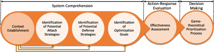

    

    Risk-based decision-support methodology for prioritization

  • what are the action sets available to the involved players given the identified context?, and

  • what are the objectives of our analysis given the identified context?

• 2) Action-Response Evaluation: This phase relies on the output of the former phase to respond to the question of “how to assess the outcomes of the different actions with respect to the identified objectives?”.

• 3) Decision Making: This phase seeks to figure out the defender’s best response. In our study, it supports the defender to tackle the pivotal question “where to start?”.

It is worth noting that our methodology defines an integrated decision-making process that glues past, present and future together. It utilizes past knowledge and experience about the system dynamics to identify a set of technically possible offensive and defensive actions. This knowledge paves the way for constructing appropriate action-response models to assess the outcomes of these different actions and behaviours under the current system configurations in order to infer the action with the best response that has to be implemented in the future towards minimizing the risk of interest (Alshawish and de Meer 2019b). The six steps are:

Step-1) Context establishment: The first step aims at understanding the system and the environment of interest. This can involve i) identifying the perimeter of the system and hence determine the scope of the analysis; ii) identifying the different components and resources relevant to the examined system and the connections among them; iii) identifying possible exposures to risks using techniques such as vulnerability assessment or organizational architecture analysis; and iv) identifying a potential target component that matters most to the system of interest. In the context of power systems, master terminal units (MTUs), Intelligent electronic devices (IEDs), data concentrator, and SCADA⁶ servers are of crucial importance for controlling and operating electric power networks since they communicate and control critical machinery and processes. The outcome of this step is a topological map of the examined system, a list of the known vulnerabilities of the system components, and their CVSS-based characteristics such as the “Attack Vector” (AV) and “Attack Complexity” (AC) metrics. These data, denoted as $\mathcal {SQ}$, represent the “status quo” of the system before implementing any remediation action. Note that “Context establishment” is a prerequisite step for other steps⁷ within the first phase “System Comprehension” as illustrated in Fig. 1. In this step, a comprehensive system analysis has to be performed. This process usually dictates the involvement of many experts with different domains of expertise. The knowledge collaboratively acquired from several experts can be further vetted to determine its accuracy and usefulness. Therefore, incorporating the expertise of several experts has positive effects with regard to (i) knowledge completeness, as well as (ii) quality and reliability of the acquired knowledge.

Step-2) Identification of potential attack strategies: The attack (or compromise) strategies represent a set of entry points to the examined network and their corresponding (feasible) compromise paths. These paths can be used by a remote adversary to reach the identified target. Based on the topological map delivered by Step-1, we can model the possible attack strategies using asset-centric compromise graphs⁸. In a compromise graph, there are basically two node types based on the characteristics and the functionality of the corresponding physical component or subsystem: i) Network nodes that are accessible from across the Internet or from a different layer (e.g. border devices, such as routers and firewalls, are always network nodes as they can maintain connectivity between two layers); and ii) Local nodes that are only accessible locally and from nodes located in the same network layer. The target node can, therefore, be either a network node or local node based on its characteristics and connectivity pattern. Additionally, each compromise graph has one hypothetical root node (called “Launch”) representing an adversarial remote node. The transitions (or edges) of a compromise graph represent the possible compromise steps. They are classified into: i) Breach edges (or inter-layer transitions; only possible if the transition’s source and destination nodes belong to different layers and the destination is a network node), and ii) Penetration edges (or intra-layer transitions; only possible between two nodes of the same layer regardless whether they are network or local nodes). In this respect, it is worth mentioning that the involvement of experts with special domain knowledge and security skills can be of vital importance at this step to refine and simplify the final compromise graphs through discarding impractical and technically infeasible compromise paths. The output of Step-2 describes the set ${SP}_{\mathcal {A}}$.

Step-3) Identification of potential defense strategies: The defense strategies represent the different vulnerability remediation actions or security investment plans the defender is able to implement to control and mitigate the compromise risk of the system of interest. For the sake of simplicity, each set of changes and activities designed to fix and improve an individual node of the identified compromise graphs can be represented by one defense strategy as shown in “Use Case” section. Since there are some vulnerabilities without any applicable patches or workarounds, each strategy d_i is characterized by its envisaged Fix-rate(d_i). This metric is the ratio between the number of fixed vulnerabilities and the number of vulnerabilities identified in the respective node. The output of Step-3 describes $\mathcal {D}'s$ action space (${SP}_{\mathcal {D}}$).

Step-4) Identification of goals: This step aims at identifying the different (operational, legal, organizational, and/or technical) goals and their relevant key performance indicators (KPIs). Utilizing optimization techniques, the defender seeks to find the best defensive action that can keep the balance between all identified goals. Throughout this work, we focus only on minimizing the compromise risk of the system in question, quantified in terms of the presented TTC security metric. As a result, we are interested in assessing the priorities of the defense strategies identified in Step-3 with respect to their impact on risk reduction against all compromise strategies identified in Step-2.

Step-5) Effectiveness assessment: Generally, this step aims at assessing the outcomes of all possible combinations of the (defender, attacker) actions, i.e. all $(d_{i},a_{j})\in {SP}_{\mathcal {D}}\times {SP}_{\mathcal {A}}$, in terms of the goals identified in Step-4. At this phase, action-response models have to be defined leveraging different qualitative, quantitative, or semi-quantitative assessment techniques such as mathematical models, simulation, eliciting expert judgments, or using historical and statistical data. In this work, we call this step “risk assessment” as we address only one objective to be optimized, which is the risk of compromise. Our risk assessment process benefits from the stochastic TTC model described in “Stochastic TTC model” section. The model involves the use of a wide variety of observed and statistical data. That is, significant uncertainty and variability are associated with such data and can have serious impact on the TTC estimation process. As a matter of fact, single-point estimates fail to communicate comprehensive risk assessments to the interested decision makers. To address this challenge, the presented methodology incorporates an iterative TTC estimation process based on Monte Carlo simulation techniques, in which any input parameter that has inherent uncertainty is modeled using a proper probability distribution function. At each iteration, different values can be used for these parameters based on their distribution functions. In this way, the assessment outcomes will provide the decision maker with a range of possible TTC estimates and the occurrence probabilities thereof. In addition to random sampling, each iteration of the risk assessment process of a scenario $(d_{i},a_{j})\in {SP}_{\mathcal {D}}\times {SP}_{\mathcal {A}}$, includes the following steps:

• i) Identify the involved compromise graph based on a_j.

• ii) Retrieve values of some model inputs (e.g. n_H, n_L) from $\mathcal {SQ}_{d_{i}}$, which is a version of the state $\mathcal {SQ}$ locally modified according to Fix-rate(d_i). That is, suppose $\mathcal {SQ}$ states that nodes x and y have 5 and 3 high-complex vulnerabilities, respectively. If d_i fixes all vulnerabilities in node x, then the TTC model will use $\mathcal {SQ}_{d_{i}}$, in which $(x,y) \xrightarrow {n_{H}} (0,3)$.

• iii) Estimate a TTTC value of each transition in a_j through applying the model described in “Stochastic TTC model” section.

• iv) Estimate a time-to-compromise value of each identified path from node “Launch” to “T” in a_j, denoted as PTTC. A PTTC value of a specific path z is simply the sum of the TTTC estimates of its constituting transitions ct: ${PTTC}_{z} = \sum \limits _{ct \in z} {TTTC}_{ct}$.

• v) Record the obtained PTTC estimates for all identified compromise paths in the graph a_j.

Subsequently, the outcomes of all iterations are merged using several techniques (e.g. frequency histogram, kernel density estimation, or the maximum entropy method) to generate the final TTC distribution function. It is worth mentioning that the assessment results of all scenarios $(d_{i},a_{j})\in {SP}_{\mathcal {D}}\times {SP}_{\mathcal {A}}$ will be used to construct the payoff matrices of our security games, which ultimately support the sought-after prioritization decisions.

Step-6) Prioritization process of the defense strategies: This step aims at assisting the defender in arranging the possible defense strategies in the order of their risk mitigation effects. This involves an iterative process of playing security games, whose underlying model is presented in “Security game model” section. Each game supports the defender in choosing and ranking one action as dictated by the computed Nash equilibrium strategy. As a result, this process yields a chain of security games, the length of which is equal to $(|{{SP}_{\mathcal {D}}}|-1)$, where $|{{SP}_{\mathcal {D}}|}$ stands for the cardinality of the set ${SP}_{\mathcal {D}}$. We call this technique iterated prioritization of risk mitigation actions (IPRMA), while the whole process is described in Algorithm 1. We construct the first game in the chain G₁ using the complete action spaces ${SP}_{\mathcal {D}}$ and ${SP}_{\mathcal {A}}$ as well as their corresponding payoff matrix M₁, whose elements are assessed following the process defined in Step-5. The best action of G₁, denoted as $d^{*}_{1}$, will be chosen according to the probability distribution prescribed by the Nash equilibrium of G₁, i.e. $\delta ^{*}_{1}$. Then, $d^{*}_{1}$ is ranked top on the ordered action list, assigned with the highest priority to be implemented. Afterwards, the system state $\mathcal {SQ}$ is globally updated according to the envisaged remediation effects of $d^{*}_{1}$ (i.e., Fix-rate($d^{*}_{1}$)). That is, $\mathcal {SQ}$ is modified as if $d^{*}_{1}$ would really have been implemented. Then, $d^{*}_{1}$ will be removed from the possible action space ${SP}_{\mathcal {D}}$. The changes applied on ${SP}_{\mathcal {D}}$ and $\mathcal {SQ}$ result in a new and smaller game, the best action of which is assigned a lower priority than the previously removed action. This process is repeated, creating new and even smaller games, until all security actions are ranked.

Use Case

For illustrative purposes, we consider a simplified network of an electricity provider, which controls the electricity provision process basically using SCADA systems. The decision makers involved in the management operations of this system increasingly integrate IT devices into the OT space that had been designed with neither widespread connectivity nor adequate security in mind. On the one hand, this integration aims at leveraging all available resources for enhancing the grid efficiency and control. But on the other hand, it could pave the way for a broad spectrum of potential attackers, ranging from amateur (cyber) criminal to advanced terrorist and state-sponsored attackers, to take control of critical assets and operational resources. Due to technical and operational constraints of power systems, the defender has to develop a coherent patch management plan. In this respect, we apply the decision-support methodology presented in “Decision-support methodology” section to assist the defender in prioritizing possible remediation actions.

1) Context establishment: As a first step, it is necessary to conduct an analysis of the network infrastructure of the examined system. The analysis outcome is depicted in Fig. 2. It illustrates the topological map of the examined electricity provider with the different technical subsystems and the connections among them. The electricity provider operates basically two different interconnected network layers. Layer (LA) includes the most networking components that are reflecting the business and the high-level control requirements. It is composed of the traditional office workstations and servers as well as the control servers that are responsible for the high-level supervision and data acquisition of the devices located in the substation network. Based on their functions and connectivity characteristics, the devices in LA are grouped into three subsystems S1, S2, and S3 as depicted in Fig. 2. Layer (LB) provides an abstract representation of an IEC-61850-based electric substation. This layer includes three subsystems S4, S5, and S6. Subsystem S4 includes the local substation workstations and HMI devices. Subsystem S5 comprises the substation management server for managing the substation assets integrity and reliability. Subsystem S6 represents the substation controller connected to the most critical process network and primary field devices. These devices include, just to name a few, transformers, circuit breakers, and capacitor banks. Controlling and protecting these critical devices involve the use of a set of programmable devices called Intelligent Electronic Devices (IEDs). Additionally, the examined system utilizes two border devices R1 and R2 (with router and firewall functionality), to control the segregation between the whole system and the Internet as well as between the two identified layers. With regard to the accessibility type, S₃ and S₆ are Local components as they are not accessible from outside their respective layers. The other LB’s devices are Network components but not accessible from across the Internet. On the contrary, S₁, S₂, and R₁ are Network components and Internet-accessible, marked as Network ⁺ nodes. S6 is identified as the target node (T) of our study based on its key role in controlling and operating the electric distribution network. More specifically, once a remote adversary $\mathcal {A}$ gains an unauthorized access to S₆ through a cyber intrusion path, $\mathcal {A}$ has control of important devices such protective relays and circuit breakers. These devices are typically employed to protect critical and expensive assets such as transformers, generators, and transmission and distribution lines. Therefore, $\mathcal {A}$ can cause major damage and a widespread power outage by manipulating the configuration settings of these devices. Exploiting cyber vulnerabilities of power grids can result in further consequences including, but not limited to, (i) disruption of grid stability through controlling Volt-Amp Reactive (VAR) devices, thereby causing voltage and frequency fluctuations in the grid; (ii) loss of substation information essential to the reliable operation of power grids such as metering information and fault recordings; and (iii) loss or interruption of communication and control channels and thus loss of engineering and maintenance access to IEDs and remote terminal units (Barnes and Johnson 2009). In our use case, the conducted vulnerability analysis gives additionally insights on the number of vulnerabilities visible in the network, classified according to their CVSS-based characteristics; i.e. AV⁹ and AC metrics. These pieces of information are summarized in Table 2.

Fig. 2

A topological map of the studied electricity provider network

Table 2 The shared system state $\mathcal {SQ}$

2) Identification of potential attack strategies: Based on the outcome of the former step, we can identify three entry points available for a remote adversary $\mathcal {A}$ attempting to compromise the identified target subsystem. These points are the three subsystems S1, S2, and R1, which are Internet-accessible. As explained in “Decision-support methodology” section (see Step-2), each attack strategy can be modeled using a compromise graph describing the different feasible compromise paths from the respective entry point to the target. Figure 3 depicts three compromise graphs corresponding to the three possible attack strategies. The attack strategy a₁, for example, aims at exploiting the weaknesses of the border device (R1) to breach¹⁰ Layer (LA) in the first place. After establishing an initial foothold in LA, $\mathcal {A}$ has two options: i) spreading through LA to strengthen the gained foothold through penetrating an ordinary node S1, S2, or S3 and then breaching Layer LB; or ii) rushing forward towards the target through breaching a network node in Layer LB; i.e. R2, S4, or S5. As explained in “Decision-support methodology” section, technical and domain knowledge from experts can be incorporated at this stage to refine the list of paths depending on their relevance and practical feasibility. Based on such knowledge, the back transitions, such as the one from S1 to R1 in the compromise graph a₁, are obviously meaningless. In an analogous manner, the attack strategies a₂ and a₃ are established exploiting the vulnerable network nodes S1 and S2, respectively. It is worth mentioning that the involved experts consider the breach transition from S1 to S2 as technically meaningless and can not offer potential adversaries with better chances to reach the target. Therefore, we omitted this transition from the compromise graph of a₂. The compromise graphs provide a powerful and compact representations of $\mathcal {A}$’s action space. Each graph can be easily updated upon identification of new compromise steps/paths.

Fig. 3

Three compromise graphs corresponding to the identified attack strategies a₁,a₂,and a₃

3) Identification of possible defense strategies: The defender $\mathcal {D}$ has identified 8 defensive actions corresponding to the patching solutions designed to fix the known vulnerabilities in the 8 nodes of the established compromise graphs. These strategies are ${SP}_{\mathcal {D}}=\{d_{1}-R1,\; d_{2}-S1,\; d_{3}-S2,\; d_{4}-S3,\; d_{5}-R1,\; d_{6}-S4,\; d_{7}-S5,\; d_{8}-T \}$, where the strategy (d₁−R1) stands for the defense strategy d₁ dedicated to fix the known vulnerabilities in the node R1. If there are some vulnerabilities without any applicable patches or workarounds, these vulnerabilities should not be removed from the shared state $\mathcal {SQ}$ when we update their respective nodes. For the sake of simplicity, we assume here that each defense strategy is able to completely resolve all vulnerabilities visible at its respective node; Fix-rate(d_i)$= 1 \; \forall d_{i} \in {SP}_{\mathcal {D}}$.

4-5) Identification of goals and effectiveness assessment: The risk of compromise is quantified using the TTC security metric. The Monte-Carlo-simulation-based assessment process has (1000) iterations¹¹ and utilizes the model described in “Stochastic TTC model” section. For each iteration, the input parameters accept different values according to their specified distribution functions. Regarding the adversary skill level parameter, each iteration chooses a random value based on the following probability mass function (Expert: 14%, Intermediate: 33%, Beginner: 34% and Novice: 19%), which is derived from the statistical findings of an existing research work on the classification of hackers by their observed behaviors (Zhang et al. 2015). The obtained TTC distributions can be further processed to generate corresponding risk probability distributions through categorizing the TTC assessments based on a set of risk categories that is predefined and approved by the system operator and other involved stakeholders: Risk Levels ={extremely severe (10): 0(day)-14(days), very high (9): 15-28, high-to-very high (8): 29-45, high (7): 46-90, medium-to-high (6): 91-150, medium (5): 151-230, low-medium (4): 231-300, low (3): 301-360, very low-low (2): 361-540, very low (1): >540 days}. In Algorithm 1, the function assessRisk() realizes the aforementioned risk assessment process to return the payoff matrices needed for our security games.

6) Prioritization process of the defense strategies: Based on Algorithm 1, the prioritization process involves constructing a chain of 7 security games. In Table 3, we summarize the input/output associated with each of those games. The chain begins with the game G₁, which is formulated using the whole action spaces ${SP}_{\mathcal {D}}$ and ${SP}_{\mathcal {A}}$, where $|{{SP}_{\mathcal {D}}}| = 8$ and $|{{SP}_{\mathcal {A}}}| = 3$. Using the shared state $\mathcal {SQ}$ described in Table 2, the function assessRisk() computes the payoff matrix M₁ of G₁. For the sake of clarity, Fig. 4 shows the matrix M₁ used to compute the Nash equilibrium in G₁. The matrix has the shape 8×3. Each matrix element (i,j) corresponds to the comprehensive TTC-based risk assessments of the respective action combination $(d_{i}, a_{j})\in {SP}_{\mathcal {D}}\times {SP}_{\mathcal {A}}$. Figure 4 shows that the risk of compromise varies not only from one defense action to another (e.g., risk of level 10 and 9 is more probable under action d₄, as shown in the 4^th row in M₁, rather than action d₈ – regardless which compromise action is played) but also from one compromise action to another given a specific defense action (e.g., risk of level 10 and 9 is more probable under action d₂ if the attacker follows action a₁ or a₃ but not a₂. That is, even simple scenarios can be associated with a certain amount of complexity involved in answering important questions such as where to start? and what to do next?. Therefore, our approach analyzes the situation as a whole towards supporting the defender when making prioritization-related decisions.

Fig. 4

The 8×3 payoff matrix of the first game (G₁) in the chain; M₁

Table 3 A chain of stochastic security games

As Table 3 tells us, the Nash equilibrium of G₁ describes a pure equilibrium strategy, in which the action (d8−T) is the most effective action in reducing the risk of compromise under the current state $\mathcal {SQ}$. Therefore, the defender assigns the highest priority to fix the vulnerabilities visible at the target node T (i.e. S6) immediately. Based on this result, the action (d8−T) is placed at the top of the sought-after ranking and removed from ${SP}_{\mathcal {D}}$. Then, $\mathcal {SQ}$ is updated accordingly through removing all vulnerability in the target. This yields a new game G₂, which has the same attack action space but with a smaller defense action space ${SP}_{\mathcal {D}}\gets {SP}_{\mathcal {D}}\setminus \{d_{8}\}$. The game chain proceeds forwards till all the defensive actions are ranked. It is worth mentioning that the function bestAction() uses the probability distribution dictated by the Nash equilibrium of each game to draw the corresponding best action. For example, bestAction() chooses the action (d4−S3) with the probability (0.375) and the action (d6−S4) with the probability (0.625) as dictated by the mixed equilibrium strategy $\delta ^{*}_{2}$ of the game G₂. In Table 3, we show only one prioritization option by pursuing the actions with the highest probabilities, i.e. $d^{*}_{k} \gets {argmax}_{d_{i}\in {SP}_{\mathcal {D}}}\delta ^{*}_{k}(d_{i})$. Afterwards, the chain proceeds forwards until the last game G₇, which supports the decision on the prioritization of the last two actions. Ultimately, there are definitively at least two prioritization options if there is one game of the chain with a mixed equilibrium strategy. These options can be combined together in a comprehensive prioritization tree, in which the nodes are the different defense actions connected by edges that have weights representing the action probabilities as assigned by the corresponding Nash equilibria. Each tree has a hypothetical root node. The weight of each path l, starting from the root to a any leaf node in the tree, can be computed as the product of the weights of its composing edges; i.e. $w(l) = \prod _{e_{i} \in l}w(e_{i})$, where w(e_i) stands for the weight of the edge e_i that is part of the path l. With regard to our use case, Fig. 5 depicts the final prioritization tree. It includes three prioritization options: i) OptionA=d₈→d₄→d₆→d₁→d₂→d₇→d₃→d₅, ii) OptionB=d₈→d₆→d₂→d₁→d₇→d₄→d₅→d₃, and iii) OptionC=d₈→d₆→d₂→d₇→d₄→d₃→d₁→d₅ with the probabilistic weights of 0.375, 0.375, and 0.25, respectively.

Fig. 5

The decision-support tree for action prioritization

Evaluation of the prioritization options

This section aims at analyzing the results of the application of our methodology and shows the performance of the delivered prioritization options. The key goal of our presented methodology is achieved by constructing the prioritization tree depicted in Fig. 5, which supports the defender in making risk-informed decisions about the prioritization of the possible security actions. The tree represents a tremendous reduction of the decision space that the defender needs to explore. In the examined use case, our methodology ends up with 3 prioritization options out of 40320 possible prioritization variations of the 8 identified defense actions¹².

For our risk-based methodology, we are interested in investigating whether the three delivered decision options have comparatively equivalent risk mitigation effects. This analysis is achieved by utilizing the equilibrium payoffs obtained by the different games of the constructed chain. The equilibrium payoffs describe the expected risk distributions the defender can assure her/himself in the different games. To have a complete vision of the risk mitigation progress as the decision-support chain move forward, we constructed two additional games G₀ and G₈. The former delivers insights into the compromise risk distribution under the current network configuration before implementing any defense action, whereas the latter addresses the situation after all actions are performed. Broadly speaking, the three options exhibit a similar positive effect of reducing the compromise risk as the chain progresses. As shown in Fig. 6a, b, and c, the three options squeeze the risk probability mass towards the lower risk levels, in much the same manner.

Fig. 6

Comprehensive risk mitigation progress. a mitigation effects of decision OptionA. b mitigation effects of decision OptionB. c mitigation effects of decision OptionC

Unlike classical game models with scalar-valued payoffs, the outcomes of our chain are more comprehensive, thereby enabling a detailed analysis of the remediation impact of the respective options. They allow for drawing conclusions that are of utmost interest to the defender of power systems. In our use case, the defender is interested in the performance of the three decision options with respect to

• Q1) what are the average risk values expected by each game in the decision chain?;

• Q2) what is the maximal risk level that occurs in 95% and 75% of the cases in each game?; and

• Q3) what are the chances of suffering a compromise risk of the category “medium-to-high (6)” or above after each step in the chain?

The answer to the question Q1 is provided by the results depicted in Fig. 7. They show that the three decision options approximately lead to similar expected risk values over the whole chain progress. The drastic risk reduction is obtained directly by the outcome of G₁, in which the average risk is reduced from (6.429) corresponding to the level “medium-to-high” to (4.111) corresponding to the level “low-to-medium”. The answers to Q2 and Q3 are more crucial to the defender as they give insights into the impact of the three decisions on the occurrences of high-level risks. Table 4 presents detailed statistical quantities about the obtained equilibrium risk distributions. The results show that the probability of suffering from a risk at level 6 or higher is reduced from 58.75% to 9.87% when having applied the game G₁. Moreover, as can be seen from Table 4 as well, the maximal risk level in 95% cases is also reduced from 9 to 7 when having applied the game G₁. Based on the results shown in Fig. 7 and Table 4, the three options have almost similar remediation effects. More precisely, OptionA can result in a slightly better risk minimization after two steps (see G₂ effects). Nevertheless, OptionB and OptionC can compensate this difference in the third step. That is, OptionB and OptionC can contribute slightly more beneficial effects if the decision constraints allow implementing three remediation actions in sequence.

Fig. 7

The average compromise risk values of the three obtained prioritization options

Table 4 Statistical quantities of the equilibrium risk distributions of all decision-support games

Conclusion

Due to their complexity and dynamic nature, electric power networks will always have a degree of vulnerability making them attractive targets for remote adversaries with different intentions. An involved defender seeks to prioritize the possible remediation actions towards efficiently mitigating the risk of compromise stemming form exploiting vulnerabilities in such systems. In fact, even small number of actions can create a large exploration space that demands a huge effort for the defender. Unlike traditional IT defenders, who are commonly indifferent between decision options with equal expected utility (losses) even if one option might be riskier, defenders of electric power systems are more sensitive to extreme (risky) events due to the high criticality of such systems. Therefore, this work presents an integrated risk-based decision-support methodology to assist the defender in making risk-informed decisions on the action priorities. It provides a seamless integration between game theory, decision theory, and risk management. This integration addresses comprehensively the competitive nature of the decision environment, the specific risk attitude of the defender of power grids, and uncertainties inherent in risk assessments. Given several constraints, the need for prioritization is evident in electric power systems. Our risk-based prioritization approach enables the defender to quantize the remediation problem of the whole system into a finite set of manageable remediation actions. Even with scarce resources, the most critical actions will be performed first to help minimize the risk of compromise in an efficient manner.

As a future research direction, we seek to extend the TTC-based risk assessment model to address the overall attack surface of organizations, including social and organizational factors. Besides the compromise risk, decision constraints such as limited time and budget can be also integrated into the decisions-making process through defining proper action-response models. Moreover, we believe our methodology has a high degree of flexibility. Therefore, it can support the defender to address multiple target components at the same time. This can be achieved by extending the attacker action space ${SP}_{\mathcal {A}}$ to include compromise graphs of different targets. Furthermore, the same methodology can be exploited to obtain risk-based vulnerability prioritization through a proper adaptation of the space ${SP}_{\mathcal {D}}$ to address specific vulnerabilities.

References

Alshawish, A., de Meer H (2019) Prioritize when patch everything is impossible! In: 2019 IEEE 44th Conference on Local Computer Networks (LCN) (LCN 2019).. IEEE, Osnabrück. in press.
Alshawish, A, de Meer H (2019) Risk-based decision-support for vulnerability remediation in electric power networks In: Proceedings of the Tenth ACM International Conference on Future Energy Systems, 378–380.. ACM. https://doi.org/10.1145/3307772.3330157.
Barnes, K, Johnson B (2009) National scada test bed substation automation evaluation report. Tech Rep Idaho Natl Lab (INL). https://doi.org/10.2172/968658.
Berr, J (2017) WannaCry ransomware attack losses could reach $4 billion. https://www.cbsnews.com/news/wannacry-ransomware-attacks-wannacry-virus-losses/. Accessed 19 Sept 2018.
Bhajanka, P, Lawson C (2018) Implement a risk-based approach to vulnerability management. Gartner.
Bie, Z, Lin Y, Li G, Li F (2017) Battling the extreme: A study on the power system resilience. Proc IEEE 105(7):1253–1266.
BSI: Bundesamt für Sicherheit in der Informationstechnik (2018) IT-Grundschutz-Kompendium. Bundesanzeiger Verlag.
Ciapessoni, E, Cirio D, Kjølle G, Massucco S, Pitto A, Sforna M (2016) Probabilistic risk-based security assessment of power systems considering incumbent threats and uncertainties. IEEE Trans Smart Grid 7(6):2890–2903.
CVSS (2015) The Common Vulnerability Scoring System (CVSS). https://nvd.nist.gov/vuln-metrics/cvss. Accessed 19 Sept 2018.
Forbes, C, Evans M, Hastings N, Peacock B (2010) Statistical Distributions. John Wiley and Sons Ltd. https://doi.org/10.1002/9780470627242.
Gonzalez-Granadillo, G, Garcia-Alfaro J, Alvarez E, El-Barbori M, Debar H (2015) Selecting optimal countermeasures for attacks against critical systems using the attack volume model and the rori index. Comput Electr Eng 47:13–34.
Giani, A, Bent R, Hinrichs M, McQueen M, Poolla K (2012) Metrics for assessment of smart grid data integrity attacks In: 2012 IEEE Power and Energy Society General Meeting, 1–8.. IEEE. https://doi.org/10.1109/pesgm.2012.6345468.
Gianini, G, Cremonini M, Rainini A, Cota GL, Fossi LG (2015) A game theoretic approach to vulnerability patching In: Information and Communication Technology Research (ICTRC), 2015 International Conference On, 88–91.. IEEE. https://doi.org/10.1109/ictrc.2015.7156428.
IEC, 61508 (2010) IEC 61508:2010 functional safety of electrical/electronic/programmable electronic safety-related systems. International electrotechnical commission.
Leversage, DJ, Byres EJ (2008) Estimating a system’s mean time-to-compromise. IEEE Secur Priv 6:52–60. https://doi.org/10.1109/MSP.2008.9.
Maghrabi, L, Pfluegel E, Al-Fagih L, Graf R, Settanni G, Skopik F (2017) Improved software vulnerability patching techniques using cvss and game theory In: Cyber Security And Protection Of Digital Services (Cyber Security), 2017 International Conference On, 1–6.. IEEE. https://doi.org/10.1109/cybersecpods.2017.8074856.
McQueen, MA, Boyer WF, Flynn MA, Beitel GA (2006a) Time-to-compromise model for cyber risk reduction estimation. In: Gollmann D, Massacci F, Yautsiukhin A (eds)Quality of Protection, 49–64.. Springer, Boston.
McQueen, MA, Boyer WF, Flynn MA, Beitel GA (2006b) Quantitative cyber risk reduction estimation methodology for a small scada control system In: System Sciences, 2006. HICSS’06. Proceedings of the 39th Annual Hawaii International Conference On, 226–226.. IEEE. https://doi.org/10.1109/hicss.2006.405.
McQueen, MA, McQueen TA, Boyer WF, Chaffin MR (2009) Empirical estimates and observations of 0day vulnerabilities In: 2009 42nd Hawaii International Conference on System Sciences, 1–12. https://doi.org/10.1109/HICSS.2009.186.
Mell, P, Bergeron T, Henning D (2005) NIST Special Publication 800-40 - Creating a Patch and Vulnerability Management Program. Natl Inst Stand Technol. https://doi.org/10.6028/nist.sp.800-40ver2.
Mooney, CZ (1997) Monte carlo simulation. Sage Publ. https://doi.org/10.4135/9781412985116.
NVD (2017) CVE-2017-0144 Detail. https://nvd.nist.gov/vuln/detail/CVE-2017-0144. Accessed 19 Sept 2018.
NVD (2018) National Vulnerability Database U.S (NVD). https://nvd.nist.gov/. Accessed 19 Sept 2018.
Nzoukou, W, Wang L, Jajodia S, Singhal A2013. A unified framework for measuring a network’s mean time-to-compromise. https://doi.org/10.1109/srds.2013.30.
Panaousis, E, Fielder A, Malacaria P, Hankin C, Smeraldi F (2014) Cybersecurity games and investments: A decision support approach In: International Conference on Decision and Game Theory for Security, 266–286.. Springer. https://doi.org/10.1007/978-3-319-12601-2_15.
RAPID, 7 (2018) The Rapid7 Vulnerability and Exploit Database. https://www.rapid7.com/db. Accessed 3 Feb 2019.
Rass, S, König S, Schauer S (2015) Uncertainty in games: Using probability-distributions as payoffs In: 6th International Conference on Decision and Game Theory for Security, 346–357.. Springer. https://doi.org/10.1007/978-3-319-25594-1_20.
Rass, S, König S, Schauer S (2016) Decisions with uncertain consequences-a total ordering on loss-distributions. PLoS ONE 11(12):0168583. https://doi.org/10.1371/journal.pone.0168583.
Rass, S, König S (2017) R Package ’HyRiM’: Multicriteria Risk Management using Zero-Sum Games with vector-valued payoffs that are probability distributions. Austrian Inst Technol (AIT). https://hyrim.net/software/. Accessed 3 Feb 2019.
Shelar, D, Amin S (2016) Security assessment of electricity distribution networks under der node compromises. IEEE Trans Control Netw Syst 4(1):23–36.
Von Neumann, J, Morgenstern O (2007) Theory of games and economic behavior (commemorative edition). Princeton university press.
Souppaya, M, Scarfone K (2013) NIST Special Publication 800-40 - Guide to Enterprise Patch Management Technologies. Natl Inst Stand Technol. https://doi.org/10.6028/NIST.SP.800-40r3.
Zhang, X, Tsang A, Yue WT, Chau M (2015) The classification of hackers by knowledge exchange behaviors. Inf Syst Front 17(6):1239–1251.
Zhang, Y, Wang L, Xiang Y, Ten C-W (2015) Power system reliability evaluation with scada cybersecurity considerations. IEEE Transactions on Smart Grid 6(4):1707–1721. https://doi.org/10.1109/TSG.2015.2396994.
Acknowledgements
Not applicable.
Funding
This work is part of the research of the “Internetkompetenzzentrum Ostbayern” funded by the Bavarian Ministry of Economic Affairs, Regional Development and Energy.
Author information
Authors and Affiliations
Contributions
AA has made contributions to conception and design, acquisition of data, analysis, interpretation of data and writing the manuscript. HM has been involved in revising the manuscript appropriately. Both authors read and approved the submitted manuscript.
Corresponding author
Ethics declarations
Competing interests
The authors declare that they have no competing interests.
Additional information
Publisher’s Note
Springer Nature remains neutral with regard to jurisdictional claims in published maps and institutional affiliations.
Rights and permissions
Open Access This article is distributed under the terms of the Creative Commons Attribution 4.0 International License (http://creativecommons.org/licenses/by/4.0/), which permits unrestricted use, distribution, and reproduction in any medium, provided you give appropriate credit to the original author(s) and the source, provide a link to the Creative Commons license, and indicate if changes were made.
About this article
Cite this article
Alshawish, A., de Meer, H. Risk mitigation in electric power systems: Where to start?. Energy Inform 2, 34 (2019). https://doi.org/10.1186/s42162-019-0099-6
Received:
Accepted:
Published:
DOI: https://doi.org/10.1186/s42162-019-0099-6