


1. Introduction
Global warming over the last decades has been well documented (IPCC, Reference Stocker, Qin, Plattner, Tignor, Allen, Boschung, Nauels, Xia, Bex and Midgley2013, Reference Masson-Delmotte, Zhai, Pörtner, Roberts, Skea, Shukla, Pirani, Moufouma-Okia, Péan, Pidcock, Connors, Matthews, Chen, Zhou, Gomis, Lonnoy, Maycock, Tignor and Waterfield2018), and its effects are particularly evident in mountainous regions (Beniston and others, Reference Beniston, Diaz and Bradley1997; Pepin and others, Reference Pepin2015), and especially in the European Alps, where temperatures are increasing more than the global average (Böhm and others, Reference Böhm2001; Auer and others, Reference Auer2007; Brunetti and others, Reference Brunetti2009). This makes Alpine regions vulnerable to changes in the hydrological cycle and to decreases in snow and glacier cover (WGMS and NSIDC, 2012; IPCC, 2019). The recent increase in temperatures has turned mountainous areas into progressive deglaciations, since glaciers have a sensitive response to climate variations through changes in volume and geometry (Oerlemans, Reference Oerlemans2001; Zemp and others, Reference Zemp2015; Huss and others, Reference Huss2017). Solid information on past climatic conditions can be provided by recognized sensitive indirect (e.g. glacial extent and glacier length) and direct (e.g. mass balance) climate proxies (Lowe and others, Reference Lowe2008; Ivy-Ochs and others, Reference Ivy-Ochs2009; Baroni and others, Reference Baroni2017b). However, very few long-term and annually resolved series of measurements of past glacial mass-balance variations extending beyond the past few decades exist but, since the annual mass balances of glaciers are mainly influenced by climatic factors (Oerlemans, Reference Oerlemans2001; Zemp and others, Reference Zemp2015), other proxies sensitive to the same factors may be used for the reconstruction of past mass-balance series. For instance, the variability of summer and annual balance is closely related to temperatures during the ablation period (Zemp and others, Reference Zemp2015; Carturan and others, Reference Carturan2016; Huss and others, Reference Huss2017). Thus, proxies sensitive to mean temperatures of the ablation season can be used to extend glacier summer balance records back in time in areas like the Italian Alps, where the latter parameter is mainly influenced by temperature (Carturan and others, Reference Carturan2016).
Several studies have successfully used tree-ring proxies to reconstruct past temperature variabilities (Büntgen and others, Reference Büntgen, Esper, Frank, Nicolussi and Schmidhalter2005; Wilson and others, Reference Wilson2016; Anchukaitis and others, Reference Anchukaitis2017; Esper and others, Reference Esper2018), as well as glacial mass-balance fluctuations in North America, Fennoscandia and the European Alps (Nicolussi, Reference Nicolussi1995; Watson and Luckman, Reference Watson and Luckman2004; Larocque and Smith, Reference Larocque and Smith2005; Linderholm and others, Reference Linderholm, Jansson and Chen2007; Leonelli and others, Reference Leonelli, Pelfini, D'Arrigo, Haeberli and Cherubini2011; Wood and Smith, Reference Wood and Smith2013, Reference Wood and Smith2015). For instance, Watson and Luckman (Reference Watson and Luckman2004) used a tree-ring width (TRW) chronology from mixed conifers (Larix lyallii Parl., Picea engelmannii Parry ex Engelm. and Pinus albicaulis Engelm.) to build a model explaining ~40% of the observed summer mass balance of the Peyto Glacier (Canada). Similarly, Linderholm and others (Reference Linderholm, Jansson and Chen2007) used tree-ring density (MXD) and TRW from the Scots pine (Pinus sylvestris L.) to reconstruct the summer mass balance of Storglaciären in Sweden and they succeeded in explaining ~50% of the observed variance. Studies in the European Alps have attempted to reconstruct annual glacier mass balances. In the Ötztaler Alps (Austria), Swiss stone pine (Pinus cembra L.) tree-ring chronologies were used to infer variations in the Hintereisferner (Nicolussi, Reference Nicolussi1995), but in the Rhaetian Alps (Italy), no stable association could be found between TRWs from the same species and climate nor annual glacial mass balances (Leonelli and others, Reference Leonelli, Pelfini, D'Arrigo, Haeberli and Cherubini2011).
The selection of proxies for reconstructing past glacial variations is fundamental. Several tree-ring parameters can be used to infer past climatic variations, such as TRW, MXD, blue intensity and stable isotopes (Schweingruber, Reference Schweingruber1988; Robertson and others, Reference Robertson, Leavitt, Loader and Buhay2008; Björklund and others, Reference Björklund2019). MXD usually gives higher correlations with mean summer temperatures since this parameter is less prone than TRW to non-climatic interferences (Briffa and others, Reference Briffa, Osborn and Schweingruber2004; Kirdyanov and others, Reference Kirdyanov, Vaganov and Hughes2006; Büntgen and others, Reference Büntgen2011; Konter and others, Reference Konter, Büntgen, Carrer, Timonen and Esper2016; Ljungqvist and others, Reference Ljungqvist2020). A higher correlation between MXD and temperature compared to TRW was demonstrated for the European larch (Larix decidua Mill.) (Büntgen and others, Reference Büntgen, Frank, Nievergelt and Esper2006) and the Scots pine from different regions (Gunnarson and others, Reference Gunnarson, Linderholm and Moberg2011; Linderholm and others, Reference Linderholm, Björklund, Seftigen, Gunnarson and Fuentes2015). However, the density analysis of the Swiss stone pine, which, in addition to the larch, characterizes the treeline in Alpine ranges, has been widely overlooked. In fact, only the width of the tree-rings (i.e. total ring, earlywood and latewood widths) has been used when assessing the association of this species with temperatures and glacial frontal variations (Nicolussi, Reference Nicolussi1995; Oberhuber, Reference Oberhuber2004; Carrer and Urbinati, Reference Carrer and Urbinati2006; Leonelli and others, Reference Leonelli, Pelfini and Cherubini2008).
The aim of this paper is to explore the possibility of reconstructing the summer mass balance of the Careser Glacier in the Rhaetian Alps using the Swiss stone pine MXD, which has recently shown to be sensitive to mean temperature during the whole ablation season (May–September; Cerrato and others, Reference Cerrato2019). The measured annual mass balance of the Careser Glacier was selected as predictand due to the length of this time series, which (i) permits a higher degree of freedom during calibration of the models; and (ii) covers the last glacier advance recorded in the Alps during the 1970s and 1980s. The MXD-based reconstructions were also compared to an independent reconstruction obtained by means of instrumental temperatures. Additionally, the instrumentally measured winter precipitation was used as an independent predictor to infer the winter mass balance and to reconstruct the full annual mass-balance record back to 1811/12.
2. Study area
This study focuses on the Careser Glacier, which is located in the Ortles-Cevedale Group of the southern Italian Rhaetian Alps (Fig. 1). The Alpine Arch is described as a transitional region characterized by at least three climatic zones (Atlantic in the West, Mediterranean in the South and European continental in the North), and the topographic effects have a relevant influence over these zones (Auer and others, Reference Auer2007). Along the chain, a strong latitudinal pattern is noticeable where the wetter zones are distributed along the southern and northern rims (Isotta and others, Reference Isotta2014). The elevation highly contributes to this precipitation pattern by sheltering the inner portion of the mountain range from the moisture-carrying winds, thus inducing the so-called ‘inner dry Alpine zone’.
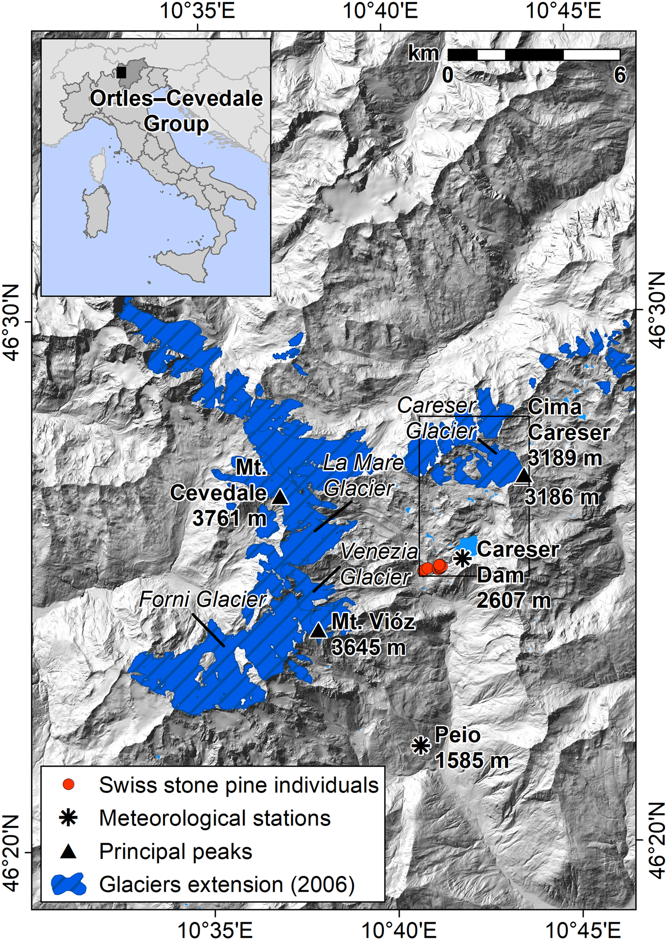
Fig. 1. Location map of the study area. For the colour image, please refer to the online version of this paper.
On the southern margin of the Alps, the climate regime changes significantly over a relatively short distance. In fact, from a climate described as temperate, according to the Köppen–Geiger classification (Peel and others, Reference Peel, Finlayson and McMahon2007), which is without a dry season but with hot summers (Cfa) observed in the Po plain, the climate conditions become typical of a Polar tundra (ET) at the highest peaks. The Ortles-Cevedale Group is located southward to the ‘inner dry Alpine zone’ (Isotta and others, Reference Isotta2014). The recorded precipitation quantity increases to the south and with elevation. A total annual precipitation of 1300–1500 mm has been estimated at 3000–3200 m a.s.l. in the area of the Careser Glacier (Carturan and others, Reference Carturan, Dalla Fontana and Borga2012), whereas the meteorological station of the Careser dam (2606 m a.s.l.) reports a mean annual precipitation of 1200 mm during the 1961–90 period (Fig. S1 in Supplementary Material).
The Careser Glacier (46.45202°N, 10.71700°E) is a mountain glacier located in the south-eastern portion of the Ortles-Cevedale Group (southern Rhaetian Italian Alps), which is the largest glaciated mountain group of the Italian Alps (Carturan and others, Reference Carturan2013b; Salvatore and others, Reference Salvatore2015). The glacier represents a unique case in the Italian Alps, owing to its long-term measured mass-balance continuous series of more than 40 years, and to the front variation fragmented series starting in 1897. Nowadays, the glacier is nested in a wide, south-facing cirque surrounded by metamorphic rock peaks (micaschists and phyllites). The glacier presents a rather flat surface, covering an area of 1.63 km2 in 2012. Recently, this glacier has been divided into three main ice bodies and three smaller ice patches caused by accelerated decay, but this effect is only the last expression of a long-term retreatment that started at the end of the 19th century (Carturan and others, Reference Carturan2013a). The glacier's winter mass balance is mainly associated with precipitation and wind-drifted snow, whereas avalanches and topographic shading are of minor importance. In contrast, the summer mass balance is mainly driven by mean temperatures of the May to September period (Carturan and others, Reference Carturan2013a; Baroni and others, Reference Baroni, Bondesan, Carturan and Chiarle2018).
3. Materials and methods
3.1 Tree-ring data
Tree-ring sampling of Swiss stone pine was performed at the treeline between 2075 and 2350 m a.s.l. in the Upper Peio Valley, which is close to the Careser Glacier (46°25.2′N, 10°41.1′E, Fig. 1). The sampling area is close to the boundary of the natural distribution range of the species (http://www.euforgen.org/species/pinus-cembra/ accounting for 2 February 2020). The fronts of the major glaciers in the area are near the tree sampling area, since the Careser Glacier is ~3 km to the northeast, while the Venezia and La Mare glaciers are ~5 km to the west. In this area, individual Swiss stone pines are scattered in a treeline ecotone where ericaceous species are dominant (Rhododendron ferrugineum L., Vaccinium spp., Andreis and others, Reference Andreis, Armiraglio, Caccianiga, Bortolas and Broglia2005; Gentili and others, Reference Gentili, Armiraglio, Sgorbati and Baroni2013), growing on immature and thin podzols, histosols and umbrisols (Galvan and others, Reference Galvan, Ponge, Chersich and Zanella2008). The trees are located in an area characterized by steep slopes, which prevent the possibility of thick snow accumulation. Moreover, the general south-oriented aspect of the area shields the trees from northerly winds, thus reducing the impact of frost desiccation (Oberhuber, Reference Oberhuber2004; Carturan and others, Reference Carturan, Dalla Fontana and Borga2012; Cerrato and others, Reference Cerrato2019).
We sampled 24 tree cores from the 12 dominant Swiss stone pines that were closest to the Careser Glacier (Fig. S2 in Supplementary Material), and these samples were processed according to standard techniques (Schweingruber and others, Reference Schweingruber, Fritts, Bräker, Drew and Schär1978; Schweingruber, Reference Schweingruber1988). The MXD data were obtained by means of an ITRAX multiscanner, following the protocol of Gunnarson and others (Reference Gunnarson, Linderholm and Moberg2011). The individual MXD series from each tree were standardized using data-adaptive age-dependent spline smoothing with 50 years of stiffness and a signal-free approach to obtain an MXD site chronology (Melvin and others, Reference Melvin, Briffa, Nicolussi and Grabner2007). The detailed description of the tree-ring dataset is reported in Cerrato and others (Reference Cerrato2019).
3.2 Glaciological and meteorological data
The annual mass balance (B n) of the Careser Glacier has been continuously measured since 1967 (Zanon, Reference Zanon1992; Carturan and others, Reference Carturan2013a; Baroni and others, Reference Baroni, Bondesan, Carturan and Chiarle2018) using the direct glaciological method (Østrem and Brugman, Reference Østrem and Brugman1991). Measurements of the winter and summer balances (hereafter, B w and B s respectively) are performed separately, since the transition between the accumulation and ablation seasons is distinct. The latter season spans from May to September, as described in detail by Carturan and others (Reference Carturan2013a). However, seven non-contiguous years (1979/80, 1980/81, 1985/86, 1986/87, 1998/99, 1999/2000, 2001/02) of seasonal mass-balance measurements are missing (Carturan and others, Reference Carturan2013a; Baroni and others, Reference Baroni, Bondesan, Carturan and Chiarle2018). To estimate the missing data in the seasonal dataset, the B s values were inferred from the B n by means of a single linear regression, which was possible since the Careser Glacier B s, as a single regressor, explains 89% of the B n variance, while the relative importance of this variable in a multiple regression is 83%. The estimated B w values were calculated as the difference between B n and the inferred values of B s. Estimating B s (and B w) from B n was preferred to estimating these values from temperature, since B n explains a higher fraction of the B s variance compared to temperature (89 vs 74%, respectively).
Long-term monthly temperature (T) and precipitation (P) series were reconstructed for the Careser Glacier site by exploiting the long meteorological series available for the Alpine region over the periods of 1774–2017 and 1800–2017 for T and P, respectively (Brunetti and others, Reference Brunetti2012, Reference Brunetti, Maugeri, Nanni, Simolo and Spinoni2014; Crespi and others, Reference Crespi, Brunetti, Lentini and Maugeri2018). The meteorological data were interpolated at the glacier site using the anomaly method (New and others, Reference New, Hulme and Jones2000; Mitchell and Jones, Reference Mitchell and Jones2005), as described in Brunetti and others (Reference Brunetti2012, Reference Brunetti, Maugeri, Nanni, Simolo and Spinoni2014) and Crespi and others (Reference Crespi, Brunetti, Lentini and Maugeri2018). For the present work, climatic data between 1811/12 and 2012/13 were considered for analysis with the overlapping tree-ring series.
3.3 Tree-ring, climatology and mass-balance correlations and reconstructions
Considering the glacier seasonal mass-balance series of the Central European region (thus including the Pyrenees and the Apennine glaciers) over the 1950–2010 period, the influence of B w on B n is limited, explaining 6% of the annual average variance (Zemp and others, Reference Zemp2015). However, in the southern Rhaetian Alps, the B w of the Careser Glacier explains ~17% of B n variability, although most of the annual variance can be explained by B s (83%) over the 1967–2010 period (Carturan and others, Reference Carturan2013a, Reference Carturan2013b). Thus, an annual mass-balance reconstruction of this particular glacier based on a summer temperature-sensitive proxy, such as TRW or MXD, would provide a biased result and, consequently, a B n reconstruction based on independently reconstructed B s and B w values was preferred.
Since avalanche contributions and winter ablation can be considered negligible (Carturan and others, Reference Carturan2013a), the precipitation amount during the accumulation period (October to May) was used as a predictor of B w (predictand) in the linear regression and scaling model. Scaling is a methodology used in dendroclimatology to reconstruct temperature variations (e.g. Esper and others, Reference Esper, Cook and Schweingruber2002), and it equalizes the mean and std dev. of a proxy to the values of a time series record over a defined period of overlap (Esper and others, Reference Esper, Frank, Wilson and Briffa2005).
Two reconstructed B s series were calculated using the interpolated temperature and the MXD data as predictors, respectively, and the measured B s as predictand in simple linear regression and scaling models. The Swiss stone pine MXD data can be used to reconstruct B s, by exploiting the strong correlation that both variables show with the mean temperature of the May to September period (MJJAS hereafter; Carturan and others, Reference Carturan2013a; Cerrato and others, Reference Cerrato2019). A linear regression model between MXD data and B s has been successfully applied to reconstruct the B s of a Scandinavian glacier using Scots pine MXD (Linderholm and others, Reference Linderholm, Jansson and Chen2007). The reconstructed B n series were obtained by adding the reconstructed scaled (or regressed) B w and scaled (or regressed) B s values for each mass-balance year, since the beginning of the MXD data series in 1811/12 to 1966/67, when glaciological measurements were started. The B n obtained as the sum of the B s reconstructed by the interpolated temperature and the B w reconstructed using precipitation is identified as ‘temp/prec-based B n’ hereafter; the B n obtained as sum of the B s reconstructed by MXD and B w reconstructed using precipitation is identified as ‘MXD/prec-based B n’.
It has been argued that for both MXD and B s, the relationships with temperature have changed very recently (Carturan and others, Reference Carturan2013a; Cerrato and others, Reference Cerrato2019). Thus, an evolutionary split-sample approach was used to check the stability of B s scaling and linear regression models, testing time windows from a length of 20 years (1967–1986) to a length of 46 years (1967–2012) with a 2-year step. The models were tested by using half of the window data to calibrate the coefficients, while the remaining data were used for validation. The quality of the correlations between MXD and temperatures, B s and temperatures, and B w and precipitation was evaluated using Pearson's correlation index (r), Spearman's correlation index (ρ), root mean squared error (RMSE) and mean absolute error (MAE). Furthermore, the difference in the calculated RMSE between the calibration and validation windows (calculated as δRMSE = RMSE[calibration] − RMSE[validation]) and the difference between the δRMSEs of each split-sample procedure (calculated as ΔRMSE = δRMSE[1st half as calibration] − δRMSE[2nd half as calibration]) were analysed to evaluate the differences in RMSE among the different windows considered for calibration (from Tables S1 to S6 in Supplementary Material). Before calculating the coefficients of the scaling (or regression) models, the correlations between predictors and predictands, and their stability, were tested for the entire 1967–2013 period, using a moving correlation analysis with a moving window of 22 years and a step of 1 year.
To test the influence of the high- and mid-frequency domains on the total correlation values between the reconstructed and the measured B n, a Gaussian-filtered series was calculated (window length = 30 years, sigma = 5 years) and used as mid-frequency series. High-frequency variability was calculated as the residual between the annual values and the mid-frequency series for both the reconstructed and the measured B n. Finally, to test the reliability of the reconstructed series, a comparison was performed with the temp/prec-based B n reconstruction of the Careser Glacier and with two B n series of other glaciers in the Alps, for which the data exceed those of the Careser Glacier measured B n (i.e. the Claridenfirn and Silvretta Glaciers, Huss and others, Reference Huss, Dhulst and Bauder2015; WGMS, 2017). Our test was based on the knowledge that, in the Alps, B n shows high consistency over large distances, although B w variability shows remarkable regional differences (Huss and others, Reference Huss, Dhulst and Bauder2015). Comparisons were also performed between nine other glaciers of the area, for which measured B n series exist in the overlapping 1966/67–2012/13 period (for details on the series used, see Tables S7, S8 in Supplementary Material).
4. Results
4.1 Summer and winter mass balances
Considering the 1967–2012 period, the mean MJJAS temperatures have a strong influence both on B s and on MXD, resulting in a significant p-value <0.01 and showing a higher correlation with the former (r 2 = 0.74) than with the latter (r 2 = 0.45). The correlation between B s and MXD shows high and significant values (Figs 2a, b), indicating a relationship between the two variables (r 2 = 0.49; p-value <0.01; Table 1; Fig. 2c). However, the evolutionary split-sample procedures show an increasing difference in the obtained correlation values among B s, MXD and temperature during the calibration period compared with those obtained during the validation period in both linear regression and scaling models. The differences become more important as soon as the more recent years are included in the considered window: more precisely, the years after 1992 when considering the MXD and B s correlation (Figs S3, S6; Tables S1, S4 in Supplementary Material) and the years after 1996 when considering the B s and temperature (Figs S4, S7; Tables S2, S5 in Supplementary Material) with both reconstruction models. A sudden increase in the ΔRMSE since 2004 was clear (Figs S3, S4, S6 in Supplementary Material) in each reconstruction, with the exception of the scaling model between temperature and B s (Fig. S7 in Supplementary Material). Increase in ΔRMSE is consistent with a decrease in the moving correlation values between MXD (or temperature) and B s, calculated using a window-length of 22 years and a time-step of 1 year. We used a 22-year window because it represents the longest window that does not show large differences between the correlation values of the calibration and validation periods, as well as RMSE and MAE (Fig. 3; see Figs and Tables in Supplementary Material for details). In fact, a remarkable change in correlation values at ~1990 is noticeable (MXD~B s, MXD~temperature and temperature~B s), even if the values remain above the significance threshold of α = 0.05 for most of the considered period (Fig. 3).

Fig. 2. The MXD data plotted against the mean May to September (MJJAS) temperature (a); the summer mass balance of the Careser Glacier plotted against the mean MJJAS temperature (b); the summer mass balance plotted against the MXD data (c); and the winter mass balance plotted against the winter precipitation (October to May) (d). All plots refer to the 1966/67–2012/13 period.

Fig. 3. Explained variance (22-year window, 1-year step, centred moving average) among the MXD, Careser Glacier summer mass balance and temperature and between the Careser Glacier winter mass balance and precipitation. For the colour image, please refer to the online version of this paper.
Table 1. Summary of the explained variance (r 2) between variables (May–September temperatures and October–May precipitations) and proxies (MXD, B s and B w)

Asterisks (*) and obelisks (†) identify values that are significant at a p-value <0.001 and 0.01, respectively.
B w is correlated with the winter precipitation from October of the previous year to May of the current year, with a mean explained variance of r 2 = 0.70 (p-value <0.01; Table 1; Fig. 2d). For the moving correlation and evolutionary split-sample procedure values, RMSE and MAE do not show significant differences in any considered windows during the 1967–2012 period (Fig. 3 and Figs S5, S8; Tables S3, S6 in Supplementary Material). The relationship between B w and precipitation can be considered stable over the entire period considered (1966/67–2012/13, Fig. 3). Therefore, to be consistent with the B s models, precipitation data from the 1966/67–87/88 period were used to build regression and scaling models of B w back to 1811/12.
The statistical results of the selected 22-year window are reported in Table 2, together with the regression and scaling coefficients used. More details on other analysed windows are reported in the Supplementary Material (from Table S1 to S6).
Table 2. Summary of the calibration and verification statistics for the summer and winter mass-balance models

More details on the indexes used can be found in Fritts (Reference Fritts1976).
r 2, explained variance; RMSE, root mean squared error; δRMSE, difference between the RMSE values of the validation and calibration windows; ΔRMSE, difference between δRMSEs; B w, winter balance; B s, summer balance; ΣP w(O–M, sum of the winter precipitation from October of the previous year to May of the current year; μT s(M–S), mean summer temperature from May to September.
4.2 Annual mass-balance reconstructions
A mass-balance estimate was calculated by applying both the regression and the scaling coefficients obtained using the 1966/67–87/88 calibration period of the two independent datasets (Table 2). In fact, the B s and B w values are independent, but were both significantly correlated with B n (p-value <0.05). The reconstructed B s, B w and B n showed good numerical and visual agreement with the measured balance series, capturing the long-term overall trend and the inter-annual variability, despite a tendency for the regression-based reconstructed balance to underestimate the measured B n and B s variance in comparison to the scaling-based reconstruction (Fig. 4).

Fig. 4. Regression and scaling inferred mass balances from the MXD, temperature and precipitation and measured mass balances of the Careser Glacier (referred to the 1966/67–2012/13 period); B w: winter (a); B s: summer (b) and B n: annual (c) mass balance. For the colour image, please refer to the online version of this paper.
The reconstructed B n series based on MXD data reproduced the observed data with scaling and with the regression model quite well (Fig. 4). Both models reached a correlation value of r = 0.73 over the entire 1966/67–2012/13 period (r 2 = 0.53); instead, the correlation values between the measured and reconstructed B n in the high- and mid-frequency domains were r = 0.49 (r 2 = 0.24) and r = 0.89 (r 2 = 0.79), respectively (Table 3). Considering only the calibration period characterized by the higher correlation values (1966/67–87/88), the correlation values increased to r = 0.61 (r 2 = 0.37) and r = 0.92 (r 2 = 0.85) for the high- and mid-frequency domains, respectively (the differences between scaling and regression were neglectable, see Tables S7, S8 in Supplementary Material). In comparison, the temp/prec-based B n reconstruction over the whole period showed higher correlation values equal to r = 0.87 (r 2 = 0.76) with both scaling and regression models; instead, when considering high- and mid-frequencies separately, the correlation values were equal to r = 0.80 (r 2 = 0.64) and r = 0.94 (r 2 = 0.88). Considering only the calibration period, the obtained correlation values were r = 0.84 (r 2 = 0.71), r = 0.83 (r 2 = 0.69) and r = 0.87 (r 2 = 0.74) for the reconstructed series and the high- and mid-frequencies (Table 3).
Table 3. Pearson's correlation values between the measured annual balance of Alpine glaciers and both the measured and reconstructed Careser Glacier B n values over the 1966/67–2012/13 period

The values in brackets refer to the 1914/15–65/66 period for the Claridenfirn (n = 52) and to the 1918/19–65/66 period for the Silvretta Glacier (n = 48). Neglectable differences in correlation values were obtained by the regression and scaling models; thus, the results were not discerned.
The comparison between the reconstructed B n of the Careser Glacier and the B n of the Claridenfirn (n = 52) and Silvretta Glacier (n = 48) shows discrete agreement in both the high- and mid-frequency domains, considering both MXD/prec-based and temp/prec-based reconstructions with both scaling and regression models (Fig. 5; Table 3). Comparisons of the overlapping periods of measured B n with other glaciers in the area are reported in Table 3 and in the Supplementary Material (Fig. S9).

Fig. 5. Z-score values of the high-frequency domain (a and d), mid-frequency domain (b and e) and whole series (c and f) of reconstructed B n values (MXD/prec-based B s plus precipitation-based B w, labelled as ‘MXD/prec B n’, and temperature-based B s plus precipitation-based B w, labelled as ‘temp/prec B n’) for the Careser Glacier obtained using the scaling models and Z-scores of the measured B n of the Claridenfirn and Silvretta glaciers. The periods considered are 1966/67–2012/13 (left column) and 1910/11–2012/13 (right column). The Z-scores of the regression models are not reported because they were very similar to the Z-scores of the scaling models. For the colour image, please refer to the online version of this paper.
The MXD/prec-based and temp/prec-based B n reconstructions returned similar trends for most of the period, with the exception of the 1890–1920 window that alone accounted for ~58% of the total differences (Fig. 6), as also attested by the series highlighting the greatest differences in these decades. The series of differences show the absence of a statistically significant trend in the differences of the scaling model and a slightly significant trend for the regression model (Figs 6c, d). These outcomes are consistent with the 5-year running means of the reconstructed and measured B n series that show good agreement until 1966/67, and with the measured B n until 1994/95. After this year, the discrepancies become more important (Fig. 7).

Fig. 6. Cumulative reconstruction of the Careser Glacier annual mass balance (B n) for the 1811/12–2012/13 (a) and 1966/67–2012/13 periods (b). The arbitrary zero was set at the year 1966/67, when direct measurements began. Plot of the differences between the MXD/prec- and temp/prec-based B n reconstructions using scaling (c) or regression (d) models. For the colour image, please refer to the online version of this paper.

Fig. 7. The calculated Careser Glacier B s and B w mass balances for the 1810/11–1965/66 period and the measured record for the 1966/67–2012/13 period for scaling (upper panels) and regressing (lower panels), respectively. The lines represent the B n 5-year running means. For the colour image, please refer to the online version of this paper.
The MXD/prec-based reconstructed B n obtained by the scaling (regression) model shows 37 (24) years with positive values during the 1811/12–1965/66 period, and increases to 41 (26) including the period for which the measured series exists (1811/12–2012/13); meanwhile, temp/prec-based reconstructed B n values show 50 (44) positive values during the 1811/12–1965/66 period, and increase to 55 (48) when also considering the 1966/67–2012/13 period. Of these positive values, 41% (42%) occurred during the 1811/12–49/50 period and 12% (8%) occurred during the 1960/61–79/80 period when considering the MXD/prec-based B n reconstruction. Of the positive values reported by the temp/prec-based B n reconstruction, 35% (38%) were highlighted during the 1811/12–49/50 period and 11% (10%) during the 1960/61–79/80 period.
On decadal timescales, the MXD/prec-based as well as the temp/prec-based reconstructed B n show some periods with a slightly positive mass balance interrupting the general negative B n trend. The periods with positive mass balances were: (i) from 1811/12 until the 1850s; (ii) in the ninth decade of the 19th century for the MXD/prec-based values, which extends to the 1910s, when considering the temp/prec-based B n; (iii) during the second decade of the 20th century; and (iv) during the 1970s (1974/75–79/80). In contrast, periods with accentuated negative mass balances occurred: (i) in the 1904/05–10/11 period; (ii) during the second half of the 1940s; (iii) since 1986/87 (Fig. 7).
5. Discussion
On the basis of MXD-based and temperature-based reconstructions of B s and the independently reconstructed B w, Careser Glacier B n estimates were calculated back to 1811/12. The higher correlation value between the B s and B n than between B w and B n for all the considered subperiods reported in Table 4 suggests that B s was the main factor influencing the Careser Glacier annual mass balance before the start of glaciological measurements, at least on the long-term timescale. However, the significant correlation between B w and B n highlights the need for using independent proxies to reconstruct both seasonal balances (Table 4). The higher importance of B w relative to B n at the Careser Glacier is demonstrated by its higher correlation value (rB wBn = 0.49, note that in Table 1 values are reported as r 2), compared to the importance of the seasonal mass-balance series of other Central European glaciers relative to their B n values (r BwBn = 0.24, Zemp and others, Reference Zemp2015). This can be ascribed to the particular climatic conditions and to the shape of the Careser Glacier that yield autumn to spring precipitation as a more important factor. The Careser Glacier's location at the southern margin of the ‘inner dry Alpine zone’ enables the glacier to benefit from the absence of an evident dry season, with large amounts of precipitation occurring during the accumulation period (Isotta and others, Reference Isotta2014; Crespi and others, Reference Crespi, Brunetti, Lentini and Maugeri2018). Additionally, owing to the shape of the glacier, feeding by snow avalanches and reduced melting caused by topographic shading are largely negligible (Carturan and others, Reference Carturan2014). The absence of significant changes in precipitation during the accumulation season for the Careser Glacier region (Brunetti and others, Reference Brunetti, Maugeri, Monti and Nanni2006; Carturan and others, Reference Carturan2013b) confirms and enforces the idea that although winter precipitation is an important factor for annual mass balance, the mean MJJAS temperatures are the crucial factor determining positive and negative annual mass balances.
Table 4. Correlation values (r 2) between mass-balance series (measured and reconstructed B s, B w and B n obtained with the scaling model) over different periods

The asterisk (*) identifies reconstructed mass balances; the obelisk (†) identifies significant r 2 values at 95%; and the dagger (‡) identifies r 2 values significant at 99%. Italic values refer to temperature-based reconstructed B s values. For B n*: not-formatted values refer to MXD/prec-based reconstructed B n values, whereas bold values refer to temp/prec-based reconstructed B n values.
An overall good visual and statistical agreement is observed between the reconstructed and measured B n during the calibration period (1966/67–88/89). However, a decrease in the modelling skill can be seen during the most recent period (1990/91–2012/13) in all the reconstructions (Figs 3, 4, 6, 7). When the modelling skills of the applied methods are compared, the scaling models better represent the measured B n variations during the more recent period, whereas the regression models tend to return to a less-negative B n (Fig. 6). These differences can be assumed marginal when considering: (i) the similarity of the RMSE between-models, which returned the values of 0.029 and 0.023 m w.e. for MXD-based and temperature-based reconstructions, and (ii) the similarity of the RMSE within-models, which account for 0.026 and 0.020 m w.e. of differences for scaling and regression models, respectively (Table 2).
As concerns the most recent period (from 1990s to date), the differences between the most negative B s values recorded by the mass-balance measurements and the reconstructed B s values are probably due to both: the decay of the Careser Glacier (Carturan and others, Reference Carturan2013a, Reference Carturan2016) and the loss of correlation between Swiss stone pine MXD and temperature (Cerrato and others, Reference Cerrato2019), which denote non-linear behaviours of the two variables over the last three decades. Indeed, in the last 30 years, a dramatic and historically unprecedented period of negative-B n years has occurred at the Careser Glacier (Carturan and others, Reference Carturan2013a; Baroni and others, Reference Baroni2017b, Reference Baroni, Bondesan, Carturan and Chiarle2018), in the Ortles-Cevedale area (Carturan and others, Reference Carturan2013b), and at the regional and global scale (Salvatore and others, Reference Salvatore2015; Zemp and others, Reference Zemp2015; Carturan and others, Reference Carturan2016). Because of its geometry (e.g. bedrock shape and hypsography), since the 1990s the Careser Glacier has been completely below its equilibrium line altitude (ELA), lacking an accumulation area and acting as a stagnant melting block of ice, as described by Carturan and others (Reference Carturan2013b). ELA increase enhanced the ablation recorded at the Careser Glacier, which made the mass loss rates double the Ortles-Cevedale group mean rates (Carturan and others, Reference Carturan2013b), and a correlation decrease occurred between the glaciological measured B s and temperature. The recorded melt rate is also a consequence of the thinning and fragmentation of ice masses, the enlargement of rocky windows and outcrops, and the lower albedo that during the last decades affected the Careser Glacier, caused by the ELA increase (Carturan and others, Reference Carturan2013a, Reference Carturan2016). Likewise, since the 1950s, the local Swiss stone pine MXD sensitivity to the mean MJJAS temperatures (in the high-frequency domain) has also gradually decreased and approached the critical correlation values during the same period in which the Careser Glacier began to show an accelerated melting rate, approximately in the 1990s (Figs 3, 4; Cerrato and others, Reference Cerrato2019). This decrease is likely to have been induced by the rise in the mean summer temperatures (MJJAS) recorded at the sampling site (Carturan and others, Reference Carturan2013b), and also globally (IPCC, Reference Masson-Delmotte, Zhai, Pörtner, Roberts, Skea, Shukla, Pirani, Moufouma-Okia, Péan, Pidcock, Connors, Matthews, Chen, Zhou, Gomis, Lonnoy, Maycock, Tignor and Waterfield2018) it could be related to the so-called ‘divergence problem’. The loss of prediction capability by a tree species has been recorded aleatorily but ubiquitously at various latitudes and altitudes in the Northern Hemisphere, and among other causes, it is ascribed to the increasing temperature that recently may have created climatically optimal conditions for some high-altitude and high-latitude species (D'Arrigo and others, Reference D'Arrigo, Wilson, Liepert and Cherubini2008) also in the studied area (Coppola and others, Reference Coppola, Leonelli, Salvatore, Pelfini and Baroni2012; Leonelli and others, Reference Leonelli2016). This ‘divergence problem’ implies that species that were stressed by summer low temperatures in the past are less stressed nowadays, lowering their capability to react to the temperatures. However, the ‘divergence problem’ might not be the only issue affecting the most recent end of MXD chronology; other factors such as common standardization or data collection methodology may influence MXD (Cook and others, Reference Cook, Briffa, Meko, Graybill and Funkhouser1995; Björklund and others, Reference Björklund2019). As a result of the accelerated melt rate of the Careser Glacier and of the loss of sensitivity of the Swiss stone pine MXD, which biases the proxies in opposite directions, the temp/prec-based reconstructed B n series lies between the measured B n and the MXD/prec-based B n reconstruction but closer to the latter, supporting the concept that the change in Careser Glacier behaviour is the most important factor that has affected the B n series in the last years (Fig. 7).
MXD/prec-based reconstruction well agrees with the temp/prec-based reconstruction, reporting a Pearson correlation value higher than 0.60 (r 2 = 0.36) over the 1811/12–1965/66 period when considering the total and filtered frequency domain (Table 4). The different models used for the reconstruction return similar results, with the B n based on regression models showing a more contracted variance compared to the B n based on scaling models (Fig. 4). This can be interpreted as an effect of the regression functions that reduce the amplitude of the reconstructed variable by the square root of the unexplained regression variance (Esper and others, Reference Esper, Frank, Wilson and Briffa2005). Therefore, the reduction of the amplitude is more appreciable for MXD than for temperature and precipitation, since the unexplained variance of the MXD parameter is slightly higher than that of the temperature and precipitation (Fig. 4). By contrast, the scaling model maintains a homogeneous variance between the predictor and the predictand, but it must be remembered that this model tends to inflate variance errors (Esper and others, Reference Esper, Frank, Wilson and Briffa2005). Nevertheless, the differences between the diverse applied models are marginal for both MXD/prec-based and temp/prec-based reconstructions. In fact, the cumulative sum of the MXD/prec-based reconstructed B n values for the 1811/12–1965/66 period suggests a total ice melt of 75 m w.e., considering both scaling and regression models. This value is lowered to 42 and 48 m w.e. when considering the temp/prec-based B n reconstruction from the scaling and regression models, respectively. This difference of 30 ± 3 m w.e. is mainly due to the discrepancies highlighted during the first decade of the 20th century between the MXD/prec-based and temp/prec-based reconstructions, with the former reporting more negative values (Figs 6, 7). This difference might be caused by (or by a combination of) the MXD acquisition method (Björklund and others, Reference Björklund2019), by the standardization employed on the MXD data (Cook and others, Reference Cook, Briffa, Meko, Graybill and Funkhouser1995) or by the intrinsic diversity of the proxy and variable that were used to reconstruct the B n. Even if the MXD is sensitive to the mean temperatures of the summer period from May to September (Cerrato and others, Reference Cerrato2019), its value also depends on the growing season prone to length variations, and on the ablation season of the glaciers. Conversely, the mean monthly temperature has a fixed length; therefore, cold springs and/or autumns could positively affect the final B s reconstructions (also reporting positive values occurring in the years 1812/13, 1813/14 and 1815/16 when considering scaling models and in 1815/16 when considering regression; Fig. 7). Moreover, the series of differences support the fact that the diversity between the B n reconstructions is related to the characteristics of the dataset employed more than to a systematic bias like the one introduced during tree-ring series standardizations (Cook and others, Reference Cook, Briffa, Meko, Graybill and Funkhouser1995; Melvin, Reference Melvin2004). Indeed, if the loss of mid- and low-frequency (sensu Melvin, Reference Melvin2004) associated with MXD standardization had had a significant influence on the reconstruction, a significant trend in the differences should have been highlighted. On the contrary, in the investigated time period (1810/11–2012/13), the scaling reconstructions do not evidence any particular trend in the series of differences, which imply that MXD/prec- and temp/prec-based reconstructions retain the same trend. A slightly significant trend is highlighted in the series of differences related to the reconstructions obtained by the regression models, and is probably induced by the different angular coefficients used to reconstruct B n (Fig. 6, Table 2).
The general negative trend that has occurred since the middle of the 19th century (Fig. 6), generally recognized as the end of the Little Ice Age in the Alps (LIA; Ivy-Ochs and others, Reference Ivy-Ochs2009), is interrupted by the appreciably flattened or slightly positive mass balance in the MXD/prec-based B n reconstruction and temp/prec-based B n during the 1964/65–79/80 period and in the 1920s. Before the 1850/60s, the MXD/prec-based and temp/prec-based B n reconstructions show another period of positive or slightly negative mass balances, with a first and higher maximum in the 1820s and a second in the 1850s (Figs 6, 7). These periods include ~70% of the reconstructed positive B n based on MXD and on temperature with both models, and the highlighted periods perfectly match the historical evidence of stationarity or re-advances of the Italian glaciers (Baroni and Carton, Reference Baroni and Carton1990, Reference Baroni and Carton1996; Citterio and others, Reference Citterio2007; Carturan and others, Reference Carturan2013a; Salvatore and others, Reference Salvatore2015; Baroni and others, Reference Baroni, Bondesan and Mortara2016, Reference Baroni, Bondesan and Chiarle2017a, Reference Baroni, Bondesan, Carturan and Chiarle2018) and of other European Alpine glaciers (Haeberli and others, Reference Haeberli, Hoelzle, Paul and Zemp2007; Zemp and others, Reference Zemp2015). The calculated reconstructions of the B n also highlight periods characterized by accelerated mass loss during the 1860s and the 1870s, between 1927/28 and 1934/35, in the 1940s and after the 1980s (Fig. 7). These findings comply with the observed Careser Glacier data series, which shows a long-term front retreat from 1933 to 1960 based on topographic data and geodetic differences and increasing mass loss rates after 1980 (Carturan and others, Reference Carturan2013a).
The topographic data make it possible to test the reliability of reconstructions by considering the 1932/33–1958/59 period, which is not included in the calibration/verification window. During this period, rates of −0.90 and −0.78 m w.e. a−1 characterized the calculated MXD/prec-based B n obtained with the scaling and regression models, whereas values of −0.72 and −0.67 m w.e. a−1 were calculated for the temp/prec-based B n. With regard to geodetic mass balances of the Careser Glacier, a rate of −0.70 m w.e. a−1 was calculated for the 1932/33–1958/59 period (Carturan and others, Reference Carturan2013a). These values are completely comparable, considering the systematic, random and spatial integration errors affecting the glaciological method (used in calibrations) and the systematic, random and density-correction errors affecting the geodetic method, all of which combine to result in the lowest detectable bias of ~0.3 m w.e. a−1 between the two methods (Zemp and others, Reference Zemp2013; Carturan, Reference Carturan2016). Before 1932/33, there are uncertainties affecting the calculation of geodetic ice loss rates, owing to the unknown period of the Careser Glacier LIA maximum and to approximations in the reconstruction of surface topography (Baroni and others, Reference Baroni2017b). Changes in the area-elevation distribution of the glacier that are negligible between 1932 and 1959 (ELA difference <10 m, Carturan and others, Reference Carturan2013a) further complicate comparisons prior to 1932/33, because at the LIA maximum, the ELA has been estimated to be 75 m lower than the one in 1932/33, thus affecting the mass balance of the glacier and probably requiring corrections before comparisons (Paul, Reference Paul2010).
When the mid- and high-frequency trends of the reconstructed B n are compared with the measured B n values of other monitored glaciers in the Alps, each glacier appears to have its own driving processes, and therefore, generalization is difficult to accomplish in a climatically heterogeneous area like the Alps, but good correlation values are appreciable (Table 3). High correlation values in the mid-term frequency are appreciable between the proposed MXD/prec-based reconstruction and all the other B n values considered, which in some cases are even higher than those among the measured B n, especially during the 1987/88–2011/12 period (Table 3; Table S8 in Supplementary Material). These correlation values can be compared with those returned by the correlation with the temp/prec-based B n reconstruction. This finding is consistent with the highlighted non-linear response of the Careser Glacier to the increasing temperature over the last 30 years and it supports the idea that the Swiss stone pine MXD can be used as a proxy for B n reconstructions at least in the mid-frequency domain. In contrast, during the same period (1988/89–2012/13), the MXD/prec-based reconstructed B n fails to coherently represent the high frequencies deriving from the influence of the divergence between the MXD data and temperature (Table 3; Table S7 in Supplementary Material). As a matter of fact, the temp/prec-based B n reconstruction returns higher correlation values, with the other glacier B n values in the high-frequency domain over the last decades. As concerns the period before 1966/67, the correlations show good values in both the high and mid frequencies, and the discrepancies relative to the B n of the other glaciers can be ascribed to the different climatic conditions and dynamics characterizing the different ice bodies (Fig. 5).
6. Conclusions
The Swiss stone pine MXD data from the southern Rhaetian Alps are a promising tool for B s reconstruction, since this proxy is sensitive to mean temperature during the whole ablation season (May to September). The temperature signal is stable over time (Cerrato and others, Reference Cerrato2019), unlike the other often-used tree-ring parameters (i.e. TRW, Leonelli and others, Reference Leonelli, Pelfini, D'Arrigo, Haeberli and Cherubini2011). In particular, the MXD series results to be strongly, negatively correlated with the B s.
The MXD data, coupled with the B w independently inferred from precipitation observations, permitted a B n variation estimate of the Careser Glacier back to the glaciological year 1811/12. Considering the agreement observed between the proposed B n MXD/prec-based reconstruction and (i) temp/prec-based B n reconstruction, (ii) glaciological data measured and (iii) past Careser Glacier extensions, we conclude that MXD data can be used as a proxy for the B s of the Careser Glacier. Furthermore, on account of the similar trend shown by the proposed MXD/prec-based B n reconstruction and by other Alpine glaciers, and considering the extended overlap between the natural range of the Swiss stone pine and the distribution of the glaciers in the European Alps, the Swiss stone pine, MXD data can be confidently applied as a proxy also to glaciers showing an ablation season moving alongside the Swiss stone pine growing season. Although there are quite a number of parameters other than temperature and precipitation (e.g. albedo, debris covering, glacier geometry and altitudinal distribution) affecting a glacier's mass balance, our results show the potential use of Swiss stone pine MXD data as a proxy for glaciological measurements with a higher degree of confidence than TRW. Even if winter precipitation can be considered an effective limit, new promising dendrochronological findings aimed at reconstructing this climatic variable in the Alpine region (Carrer and others, Reference Carrer, Pellizzari, Prendin, Pividori and Brunetti2019) encourage further investigations on Swiss stone pine MXD as a proxy for B s. Indeed, a great advantage of this proxy is that it can cover centuries with annual resolution and thus can improve and extend our glaciological knowledge further back in time.
Supplementary material
The supplementary material for this article can be found at https://doi.org/10.1017/jog.2020.40
Data availability
The dendrochronological data are freely accessible at the NOAA International Tree-Ring Data Bank (ITRDB) at the link: https://doi.org/10.25921/y4pb-3488.
Acknowledgments
This work was financially supported by the Italian MIUR Project (PRIN 2010–11): ‘Response of morphoclimatic system dynamics to global changes and related geomorphological hazards’ (national and local coordinator: C. Baroni) and by the project of strategic interest NEXTDATA (PNR National Research Programme 2011–2013; project coordinator A. Provenzale CNR-IGG, WP 1.6, leader C. Baroni UNIPI and CNR-IGG). We thank Göteborg University, Stockholm University, the University of Pisa and the Erasmus Programme Consortia Placement traineeship program for financial support. We are also grateful to Gino Delpero, Luca Colato and Mattia Delpero of Custodi Forestali – Comune di Vermiglio and Comune di Peio (TN) for helping with field activities and sampling. We thank Fabio Angeli, who is responsible for the Ufficio Distrettuale Forestale di Malè (TN). The English text has been edited by American Journal Experts (certificate verification key: C223-B25C-189B-3977-13EP). We are grateful to the editors and the anonymous reviewers for their valuable comments to this work.
Author contributions
This study was developed with contributions from all authors: RC carried out data analysis and laboratory work for the density data under the supervision of BEG and HWL. RC performed field sampling, with contributions from CB and MCS. RC, MCS, HWL, BEG, LC, MB and CB contributed equally to the interpretation, discussion and conclusions of this paper. LC provided an updated glaciological series. MB reconstructed the instrumental meteorological data. The text was written by RC and MCS, with contributions from CB, LC, MB, HWL and BEG. The project was directed, coordinated and funded by CB.
Conflict of interest
The authors declare that they have no conflicts of interest.
Disclaimer
Any use of trade, firm or product names is for descriptive purposes only and does not imply endorsement by the involved universities.


 Open access