
Abstract
The purpose of this note is to prove the existence of a conformal scattering operator for the cubic defocusing wave equation on a non-stationary background. The proof essentially relies on solving the characteristic initial value problem by the method developed by Hörmander. This method consists in slowing down the propagation speed of the waves to transform a characteristic initial value problem into a standard Cauchy problem.
1 Introduction
1.1 The result
Consider a globally hyperbolic smooth manifold \((M,{\hat{g}})\), whose metric \({\hat{g}}\) satisfies the vacuum Einstein equations. Let \(\Sigma \) be a Cauchy hypersurface in \(M\) and T be a future-oriented timelike vector normal to \(\Sigma \). Consider the Cauchy problem for the defocusing cubic equation
where \({{\hat{\nabla }}}\) is the Levi–Civita connection associated with \({\hat{g}}\). Since \((M,{{\hat{g}}})\) is globally hyperbolic, there exists a time foliation on the manifold, and the global existence of solutions and the existence of scattering operator can be discussed for this problem. Nonetheless, since the metric is a priori not static, the standard approach to prove the global existence, for instance, through Strichartz estimates, and the existence of the scattering operator, which would require a proof of the local energy decay, might fail. The cubic wave equation (1) enjoys nonetheless good properties regarding conformal transformations. Indeed, if one considers a metric g conformal to the original metric \({\hat{g}}\)
one obtains the following identity
where \({\nabla }_\alpha \) is the Levi–Civita connection associated with g. Hence, if \({{\hat{\phi }}}\) is a solution to the problem (1), then \(\Omega ^{-1} {{\hat{\phi }}}\) is a solution to the corresponding geometric equation arising from the conformal metric g. This property can be exploited to prove the global existence of solutions to the problem (1) by considering the local existence for the conformal problem, and construct a scattering operator by relying on that operation.
Penrose introduced in the 1960s a class of space-times admitting a conformal compactification. These space-times, known as asymptotically simple space-times, model isolated bodies. The compactification is obtained by completing the manifold with two disconnected hypersurfaces, null for the conformal metric when the cosmological constant vanishes, which represent the extremities of future and past null geodesics. These hypersurfaces are denoted by \({{\mathscr {I}}}^+\) and \({{\mathscr {I}}}^-\), respectively. The strategy for the construction of the scattering operator exploiting the existence of the conformal compactification is the following. For convenience, the construction is done for smooth data with compact support.
Consider smooth compactly supported initial data \(({{\hat{\phi }}}_0, {{\hat{\phi }}}_1)\) on \(\Sigma \) for the Cauchy problem (1). These data are appropriately transformed into data \(({\phi }_0, {\phi }_1)\) for the conformal cubic wave equation:
Since the problem is now set on a space compact in time, the global existence problem for the Cauchy problem (1) turns into a much easier local existence problem (2) for the rescaled equation. The existence result of Cagnac–Choquet-Bruhat [3] can be used to address the existence in this context. The radiation profile of the function \({\hat{\phi }}\) can be obtained by considering the trace of \(\Omega ^{-1} {\hat{\phi }}\). We define the mapping, generalising the inverse wave operators:
Energy estimates can be proven for the cubic wave operator and we prove in fact
The existence of the wave operators defined on \(H^1({{\mathscr {I}}}^\pm )\), inverses of the trace operators \( \left( {\mathfrak {T}}^\pm \right) ^{-1} \), is obtained by solving the characteristic Cauchy problem for the conformal cubic wave equation with data on \({{\mathscr {I}}}^{\pm }\). The generalisation of the standard scattering operator is defined as the operator
In this paper, we prove the existence of a bi-Lipschitz conformal scattering operator, which extends the notion of scattering operator to space-times which are non-static:
Theorem
There exists a locally bi-Lipschitz operator \({\mathfrak {S}} : H^{1}({{\mathscr {I}}}^{-}) \rightarrow H^{1}({{\mathscr {I}}}^{+}) \), which associates with past radiation profiles of solutions to the problem (1) the corresponding future radiation profiles.
1.2 Conformal techniques, scattering, asymptotic behaviour
The well-posedness of the Cauchy problem for this equation, and in this geometric setting, has been addressed in [3]. The existence of a scattering operator on Minkowski space-time has been considered, on flat space-times in [15], for general semi-linear wave equations, and by conformal methods on flat space-time in [2]. The existence of a scattering operator, under more constraining assumptions, has been considered by the author in [14], and this work extends this previous work to the generic cubic wave equation. In particular, we remove an artificial assumption on the decay of the coefficient of the nonlinearity. The purpose of this assumption was to compensate for the blow-up of the Sobolev constant associated with the Sobolev embeddings of \(H^{1}\) into \(L^{6}\) in dimension 3.
Since the metric is not stationary, this geometrical setting is a priori not amenable to standard analytic techniques to prove the existence of a scattering operator. To construct this operator, we exploit the conformal invariance of the equation, in conjunction with the conformal compactification of the space-time. The rescaled solution \(\Omega ^{-1}{{\hat{\phi }}} = \phi \) can be extended up to \({\hat{M}}\) by means of Eq. (2). The trace of \(\Omega ^{-1}{{\hat{\phi }}}\) on the boundaries is the radiation profiles, in this conformal setting, discussed by Friedlander [9]. Hence, the trace operators \({\mathfrak {T}}^{\pm }\), associating with initial data for the Cauchy problem for the conformal wave equation (2) to the traces of the corresponding solutions to (2) on the boundaries \({{\mathscr {I}}}^{\pm }\), generalise the standard inverse wave operators of the classical scattering theory, see [18]. The actual existence of the scattering operator is performed by inverting the trace operators, that is to say, within the appropriate function spaces, solving the characteristic Cauchy problem with data on the boundaries of M.
Conformal methods to study global problems for partial differential equations in relativity go back to Penrose and Sachs and the peeling of higher spin fields. It was further studied in the context of the Cauchy problem in the mid-80s, early ’90s (see, for instance, [3]). Friedlander [9] pioneered scattering theory in relativity. The reader who wishes to have a more exhaustive bibliography should refer to [13, 21, 27]. In the past years, this approach by conformal techniques to understand the asymptotic behaviour of solutions of field equations in general relativity has been studied in various contexts: Mason and Nicolas [18] obtained the first analytic result for linear fields, followed by a peeling result on the Schwarzschild background, for scalar wave [19], spin 1/2 and spin 1 fields [20]. This has been later extended to nonlinear waves on Kerr black holes [25]. As mentioned before, the conformal scattering construction was extended to a nonlinear wave equation [14]. Similar constructions based on local energy estimates [23] were obtained on Reissner–Nordström black holes [22] for the Maxwell equations. More recently, the existence of a conformal scattering operator has been proven for Yang-Mills fields on the de Sitter background [30].
1.3 Description of the work
We now review the key points of the result. As already mentioned, this work is an extension of previous work [14]. We are in particular building on the estimates performed in the asymptotic spatial region \(i^0\).
The main improvement of this paper is the possibility to handle a more general nonlinearity. In the previous paper, we assumed that the nonlinearity was multiplied by a decaying function b. This restriction has its origin in the treatment of the characteristic initial value problem on \({{\mathscr {I}}}^\pm \) to construct the inverse of the trace operators \({\mathfrak {T}}^\pm \). The technique relies on a fixed point argument in the energy space obtained by foliating the interior of the light cones at infinity \({{\mathscr {I}}}^{\pm }\). Because of the power nonlinearity, Sobolev embeddings are required. Nonetheless, the volume of the leaves goes to zero, and a well-known consequence is the blow-up of the related Sobolev constant, associated with the Sobolev embedding from \(H^{1}\) into \(L^6\). The nonlinearity is multiplied by a function decaying sufficiently fast to compensate for this blow-up of the Sobolev constant.
To circumvent that issue, the strategy to approach the characteristic initial value problem is changed. In particular, this strategy avoids the use of the Sobolev embeddings on a shrinking foliation and relies on the work by Hörmander [12] for the wave equation. The principle is the following. One assumes the existence of a solution for the Cauchy problem for the considered geometric equation.Footnote 1 One considers an initial characteristic surface C. A time function being chosen to split the metric
where \(h_{\Sigma _t}\) is the Riemannian metric on the leaves of the foliation induced by the time function \((\Sigma _t)\), the propagation speed of the metric is slowed down
The initial characteristic hypersurface C becomes spacelike for \(g_{\lambda }\), and solutions to the Cauchy problem for the geometric equation associated with \(g_{\lambda }\) can be solved. In the case of the cubic wave equation, this result has been obtained by Choquet-Bruhat–Cagnac [3]. Given initial data, a family of solutions is then obtained, depending on \(\lambda \). Standard compactness arguments can then be used to prove the existence of an accumulation point as \(\lambda \) goes to one which satisfies the characteristic initial value problem. This method by Hörmander has been extended to metrics of weak regularity in [24] for the linear wave equation. This paper clarifies some points of [24]; in particular, in the way some energy estimates are performed and in the use of trace theorems for intermediate derivatives.
This technique by Hörmander can only be used in a neighbourhood of timelike infinity, where the Penrose compactification leads indeed to a compact space. Near spacelike infinity \(i^0\), the metric coincides with the Schwarzschild metric, and the chosen conformal factor does not lead to a compactification in the neighbourhood of \(i^0\). There, the existence of solutions to the characteristic initial value problem can be proven by relying on an explicit foliation. Global solutions to the Cauchy problem in the past of \({{\mathscr {I}}}^+\) (resp. the future of \({{\mathscr {I}}}^{-}\)) are obtained by appropriately gluing the different solutions to the characteristic initial value problem in the neighbourhood of \(i^\pm \) and the neighbourhood of \(i^0\).
1.4 Organisation of the paper
Section 2 contains the precise geometric framework, in Sect. 2.2, and reminders on the cubic wave equation, in Sect. 2.3, in particular, the global existence of solutions to the defocusing wave equations, see Proposition 2.2 and some estimates for the characteristic initial value problem, see Proposition 2.4. Section 3 solves the characteristic initial value problem for the cubic wave equation, by Hörmander’s method, see Theorem 3.2. Section 4 addresses the proof of the uniqueness of solutions to the Cauchy problem, see Proposition 4.5. The next section, Sect. 5, addresses the problem of solving the characteristic initial value problem, see Proposition 5.4. The global characteristic initial value problem is solved in Sect. 6. Finally, the trace operators, as well as the scattering operators, are obtained in Sect. 7, see Theorem 7.1, and its corollary, Corollary 7.2. “Appendix A” contains reminders on a trace theorem, see in particular Theorem A.1, and its use when energy estimates can be proven.
2 Geometrical and analytical preliminaries
2.1 Conventions, notations
All along the paper, the metrics have signature \((-+++)\), and we use the Einstein summation conventions. The expression \(a \lesssim b\), where a and b are two functions defined on M means that there exists a constant \(C>0\) depending on the geometry such that
If \(a \lesssim b\) and \(b \lesssim a\), then one writes \(a \approx b\).
2.2 Regular asymptotically simple space-time
Penrose introduced the concept of asymptotically simple space-times [26, Chapter 9.6] as idealised space-times modelling a spatially localised gravitational source. These space-times do not need to satisfy Einstein equation. Nonetheless, they can be conceived as resulting from a small perturbation of Minkowski space-time (when the cosmological constant vanishes), in which case they are a strong form of asymptotically flat space-times (see [8, Chapter 2.3] for further discussion). They can be obtained by combining the result of gluing by Corvino–Schoen and Chruściel–Delay [5,6,7], and the result by Andersson–Chruściel [1] on the existence of space-time with smooth \({{\mathscr {I}}}^{+}\) arising from regular enough data on a hyperboloid. Nonetheless, in the context of stability theorems of Minkowski space-times, the conformal boundary exists but it not smooth [4]. More importantly, smoothness at conformal infinity has been discarded as physically relevant for standard physical systems (see [4]). One important point of Hörmander’s method is precisely that the regularity of the initial characteristic surface could be low, see [24], though we are not working in this frame. Though it is not necessary, we assume that the Einstein equations in vacuum with vanishing cosmological constant are satisfied. In particular, the scalar curvature of the physical metric vanishes.
Definition 2.1
(Regular asymptotically simple space-times) A space-time \(({\hat{M}},{\hat{g}})\) is a regular asymptotically simple space-time if there exists a manifold with boundary M, with boundary \(\partial M = {{\mathscr {I}}}\), a Lorentzian metric g on M and a \(C^\infty \)-conformal factor \(\Omega \) such that:
- (1)
The interior of \({{\hat{M}}}\) is M.
- (2)
\({{\hat{M}}}\) is embedded in M and, on M, \( g = \Omega ^2 {{\hat{g}}}\);
- (3)
g and \(\Omega \) are \(C^\infty \) over M;
- (4)
\(\Omega \) is positive on M and \(\text {d}\Omega \ne 0\);
- (5)
Any inextensible null geodesic admits a future (resp. past) endpoint on \({{\mathscr {I}}}^+\) (resp. \({{\mathscr {I}}}^-\)).
The framework of this paper imposes the use of energy estimates to prove the existence of a solution of the Cauchy problem set up on the characteristic cones at infinity. These energy estimates usually rely on the use of Stokes’ theorem, requiring that the metric is regular enough at the tip of the cone. This is why an extra regularity assumption is made at tips of the boundary of the manifold.
Assumption 1
Let \(({{\hat{M}}},{{\hat{g}}})\) be regular asymptotically simple space-time whose conformal compactification is denoted by \(( M, g = \Omega ^2 {{\hat{g}}})\). We assume that there exist a neighbourhood \(U_1\) of \(i^0\) in M and a system of coordinates \((t, r, \theta , \phi )\) on \(U_1\cap {{\hat{M}}}\) such that, in \(U_1\cap {{\hat{M}}}\), the metric is the Schwarzschild metric
Another important assumption which is made on the structure of the asymptotically simple space-time and which is the most important restriction on the geometry:
Assumption 2
Assume that there exists a neighbourhood \(U_2\) of \(i^\pm \) in \({M}\), and an embedding of \(U_2\) into a manifold \({\bar{M}}\), such that the metric g extends to a \(C^\infty \)-metric onto \({\bar{M}}\).
2.3 Some reminders on the cubic wave equation
2.3.1 Conformal changes for the cubic wave equation
Consider the conformally related metrics \(g\) and \({{{\hat{g}}}} = \Omega ^{-2} g\). Then, it is a straightforward calculation that \({{\hat{\phi }}}\) is a solution to the cubic wave equation on the manifold \({{\hat{M}}}\)
if, and only if, on \({{\hat{M}}}\), the function \(\phi = \Omega ^{-1} {{\hat{\phi }}}\) satisfies the equation
2.3.2 Estimates for the defocusing wave equation
It should be noticed that we are working here with the defocusing wave equation. Given a time foliation \((\Sigma _t)\) on \({{\hat{M}}}\), with unit future-oriented normal T, we define the energy E(t) at time t
where D is the induced connection on \(\Sigma _t\). E(t) is approximately conserved along the evolution, in the sense that
Hence, for the defocusing wave equation, it is possible to prove global existence for large data in \(H^1(\Sigma _0)\times L^2(\Sigma _0)\).
The key tool is a Sobolev embedding from \(H^1(\Sigma _t)\) into \(L^6(\Sigma _t)\) in dimension 3. As long as these embeddings can be performed uniformly (for instance, when all the leaves are diffeomorphic to \(R^3\), or the 3-sphere), then the global existence for all data is ensured.
The strategy to perform the estimates is the following:
whenever we are working with a finite time interval, we use the standard energy estimates for the linear wave equations, similar to [28, Chapter 1, §3], where, for the local existence, \(H^s\)-norms are propagated;
we otherwise use the conservation of the energy with the nonlinear term.
2.3.3 The Cauchy problem for the cubic wave equation
The section contains some preliminary known results about the global existence of solutions to the Cauchy problem for the cubic wave equation
where \(\square = \nabla _\alpha \nabla ^\alpha \) is the wave operator associated with the metric \(g\). The well-posedness result of Cagnac and Choquet-Bruhat [3, Théorème 2] is recalled:
Proposition 2.2
Let X be a compact manifold. Consider the Lorentzian manifold \((X\times {\mathbb {R}}, g)\) so that \(X\times \{t\}\) is a family of uniformly spacelike hypersurfaces. Assume that the deformation tensor of the vector \(\partial _t\) is bounded as well as a sufficient number of derivatives of the metric. The Cauchy problem
admits a global solution in \(C^1({\mathbb {R}}, L^2(X))\cap C^0({\mathbb {R}}, H^1(X))\). Furthermore, the a priori estimate holds, for all \(t\in {\mathbb {R}}\):
Remark 2.3
We could add a function b in the equation as follows:
Cagnac and Choquet-Bruhat in [3] addressed the local well-posedness for this equation under the following assumptions on the function b: the function b is bounded on M, once differentiable function on M, admits a \(C^1\)-extension to M and, for a given future-oriented unit timelike vector field \(T^a\) on the unphysical space-time M, there exists a constant c such that
The conformal scattering operator could be constructed in that situation in a similar fashion. This extension has very little meaning in the context of that work, and its purpose, and is therefore ignored.
2.3.4 A priori estimates for the characteristic initial value problem
In previous work, we have proven various a priori estimates. Since these estimates are the basis of Hörmander’s method for solving the characteristic Cauchy problem, we recall in this section the various energy estimates which were previously proved. It is important to note that, in this previous work, as noted in [14], the a priori energy estimates are proved without the decay assumptions at the tip of the vertex on the function b, as considered in Remark 2.3.
The first result is a local a priori energy estimate in the neighbourhood of the tip of the vertex. The geometric and analytic settings are the following: let p be a point in \({{\hat{M}}}\) and U an open neighbourhood of p in M, with compact closure. Assume that one can define the past light cone \(C^-(p)\) globally in U. Let t be a time function defining a foliation \(\{\Sigma _t\}_{t= 0\cdots 1 }\) of the past of \(C^-(p)\). The unit future-oriented normal to \(\Sigma _t\) is denoted by \(T^a\) . On \(C^-(p)\), let l be a generator of future-oriented null geodesics ending up at p. Let n be a null vector field transverse to \(C^-(p)\) (see Fig. 1 for a representation with respect to a given past light cone) such that
The family (l, n) is completed into a family \((l,n,e_1, e_2)\) so that the family \((l,e_1, e_2)\) is tangent to the cone \(C^-(p)\) and \((e_1, e_2)\) is orthogonal to (l, n) . The derivatives with respect to the vectors \(e_1, e_2\) are denoted by \(\nabla _{{\mathbb {S}}^2}\).
We consider the standard Sobolev spaces on \(\Sigma _t\), \(H^1(\Sigma _t)\) and \(L^2(\Sigma _t)\). The set of smooth functions on the cone \(C^-(p)\) in the future of \(\Sigma _0\) with compact support away from the tip p is endowed with the norm:
where \(n\lrcorner \text {d}\mu [{{\hat{g}}}]\) is the contraction of the ambient four-dimensional volume form \(\text {d}\mu [{{\hat{g}}}]\) with the null vector n transverse to the light cone \(C^-(p)\). The completion for this norm of the set of smooth functions with compact support away from p is denoted by \(H^1(C^{-}(p))\). Using standard energy estimates, one gets the following proposition:
Proposition 2.4
Let \(\phi \) be a solution of the equation
The following inequalities hold:
and
Furthermore, for all t, one has
Remark 2.5
Using Sobolev embedding from \(H^1(\Sigma _0)\) into \(L^4(\Sigma _0)\) and from \(H^1(C^-(p))\) into \(L^4(C^-(p))\), one immediately gets the same inequality without the \(L^4\) norms.
3 Characteristic Cauchy problem à la Hörmander
The purpose of this section is to establish an a priori well-posedness result of the characteristic Cauchy problem for the wave equation on a curved space-time based on the result by Hörmander [12], extended in [24] and partially used in [14] to prove the existence and uniqueness of a weak solution to the characteristic Cauchy problem in \(H^1(M)\). More regularity is required when establishing the Lipschitz continuity of the wave operator. The method used by Hörmander is based on a reduction of the propagation speed of the considered wave equation so that one can resort to the standard existence result of the wave. In the following, one restricts oneself to a light cone, but the result can be extended in the same way to arbitrary weakly lightlike hypersurfaces.
The geometric setting is the following: consider a point p in M. One denotes by \(C^-(p)\) the past light cone from p. Consider a time function defined in the interior of \(C^-(p)\). The induced foliation is denoted by \(\Sigma _t\). The part of \(C^-(p)\) between \(\Sigma _0\) and \(\Sigma _T\) is denoted \(C_T\). One assumes that the slice \(\Sigma _0\) is in the past of p and the slice containing p is denoted by \(\Sigma _T\). The unit future-oriented normal vector to the time slices is denoted by \(T^a\). One considers a 3+1 splitting of the metric in the following form:
where \(h_{\Sigma _t}\) is a Riemannian metric on \(\Sigma _t\) and the lapse N is given by:
The functional setting is given by:
on the time slice \(\Sigma _t\), one defines the energy of a function \(\phi \):
$$\begin{aligned} E_\phi (\Sigma _t) = \Vert \phi \Vert ^2_{H^1(\Sigma _t)} + \Vert T^a\nabla _a\phi \Vert ^2_{L^2(\Sigma _t)}; \end{aligned}$$on the light cone \(C^-(p)\), the following \(H^1\) norm is considered:
$$\begin{aligned} \Vert \phi \Vert ^2_{H^1(C^-(p))} = \int _{C^-(p)} \left( (\nabla _l \phi )^2 + |\nabla _{{\mathbb {S}}^2}\phi |^2+\phi ^2\right) T^a\lrcorner \text {d}\mu [g] \end{aligned}$$where l is a non-vanishing generator of the null directions of \(C^-(p)\) and \(T^a\lrcorner \text {d}\mu [g]\) is the contraction of the space-time volume form with the vector field T. The space \(H^1(C^-(p))\) is defined as being the completion of the space of smooth functions whose compact support does not contain p. One also define in similar way \(H^1(C_T)\).
Remark 3.1
One could have defined, like Hörmander, \(H^1 (C^-(p))\) by transporting the \(H^1\) structure of a timelike slice on \(C^-(p)\). It happens that the two definitions coincide [14].
Consider the characteristic Cauchy problem
Note that, for the discussion of this section, the scalar curvature term is excluded from the discussion, but can be treated similarly, exploiting the fact the curvature is bounded.
The purpose of this section is to prove that there exists a strong solution to the characteristic Cauchy problem up to the hypersurface \(\Sigma _0\) in the past of p.
Using Proposition 2.2, one can then prove the following theorem:
Theorem 3.2
The characteristic Cauchy problem (2.1) admits a global strong solution down to \(\Sigma _0\) in \(C^0({\mathbb {R}}, H^1(\Sigma _\tau ))\cap C^1({\mathbb {R}}, L^2(\Sigma _\tau ))\). The following a priori estimates furthermore hold:
Proof
Assuming that there exists a solution in \(C^0({\mathbb {R}}, H^1(\Sigma _\tau ))\), the a priori estimates are a consequence of in [14, Proposition 4.15].

Extended foliation in the cylinder
The proof of the theorem will require at a point the use of Sobolev embeddings. This requires to work with an extension of the foliation \((\Sigma _\tau )\) to a cylinder. One then considers a smooth isometric embedding of \((J^-(p)\cap J^+(\Sigma _0),g)\) into a compact cylinder (U, g), see Fig. 1. The foliation \((\Sigma _\tau )\) is extended on the cylinder U in a spacelike foliation of U for the extension of the metric g. We denote by \(({\tilde{\Sigma }}_\tau )\) this extension; all the leaves of this foliation are now topological 3-spheres endowed with a Riemannian metric, and as a consequence, all the Sobolev spaces \(H^k({\tilde{\Sigma }}_\tau )\) considered on the leaf \({\tilde{\Sigma }}_\tau \) are equivalent since the leaf is compact. Furthermore, the cone \(C_T\) is extended as a weakly spacelike hypersurface \({\tilde{C}}\), which by construction is a Cauchy surface. The spacelike foliation \((\Sigma _\tau )\) is extended in the past of \({\tilde{C}}\), for values of \(\tau \) in a compact interval \(I = [a,b]\), with \(T \le b\).
We consider the initial datum \(\theta \) on \(C_T\) in \(H^1(C_T)\). This function \(\theta \) is extended as a function \({{\tilde{\theta }}}\) in \(H^1({\tilde{C}})\) (see, for instance, [29, Chapter V, Theorems 5 and 5’]) such that
where the constant C depends solely on the geometry of the boundary of \(C_T\). In particular, this constant blows up as T goes to 0.
The proof of the well-posedness relies on the method introduced by Hörmander [12] which consists in slowing down the propagation speed of the waves. A detailed proof of Hörmander’s paper is given in [24] when the metric is only Lipschitz. The following proof follows step by step this paper (and especially the scheme given in the proof of Theorem 4.3), modifying it when necessary.
The reduction of the propagation speed is realised by introducing a parameter \(\lambda \) in \(\left[ \frac{1}{2}, 1\right) \) and a family of metrics \(g_\lambda \):
so that the hypersurface \({\tilde{C}}\) becomes spacelike for the metric \(g_\lambda \).
According to Proposition 2.2, for any \(\lambda \) in \(\left[ \frac{1}{2}, 1\right) \), the Cauchy problem
admits a solution \(\phi _\lambda \) in \(C^1(I, L^2({\tilde{\Sigma }}_\tau ))\cap C^0(I, H^1({\tilde{\Sigma }}_\tau ))\) such that:
where \(c_\lambda \) is a constant which depends continuously on the scalar curvature of \(g_\lambda \). Since the interval under consideration is compact and since, as a consequence of the previous remark, \(c_\lambda \) depends continuously on \(\lambda \), one can replace \(c_\lambda \) by its supremum over \(\left[ \frac{1}{2}, 1\right) \). Furthermore, \({\tilde{C}}\) is compact and, as consequence, all the Sobolev spaces associated with a smooth metric are equivalent. This includes \(H^1({\tilde{C}})\). The family \((\phi _\lambda )_{\lambda \in \left[ \frac{1}{2}, 1\right) }\) is then uniformly bounded in \(L^\infty (I, H^1({\tilde{\Sigma }}\tau ))\):
Consider now a sequence \((\lambda _n)\) converging to 1 and one denotes by \((\phi _n)\) the associated sequence. One denotes by U the volume delimited by \(\Sigma _0\) and \(C^-(p)\).
Remark 3.3
Before studying the convergence process, let us remind the reader that, using a priori estimates of Proposition 2.4, the energy on the initial time slice \({\tilde{\Sigma }}_0\) controls all the energies on the time slices \({\tilde{\Sigma }}_\tau \) for \(\tau \in I\). As a consequence, a convergence stated for \(H^1(\Sigma _0)\) actually holds in \(L^\infty (I, H^1({\tilde{\Sigma }}_\tau ))\).
One now proceeds by extracting successively sequences of \((\lambda _n)\) as follows:
- (1)
Since \((\phi _n)\) is bounded in \(C^1(I, L^2(\Sigma _\tau ))\cap C^0(I, H^1(\Sigma _\tau ))\), \((\phi _n)\) is bounded in \(H^1(U)\). Hence, using Kakutani’s theorem, there exists a sub-sequence of \((\phi _n)\) converging weakly in \(H^1(U)\) towards a function \(\phi \) in \(H^1(U)\). Furthermore, using Rellich–Kondrachov’s theorem, since \(H^1(U)\) is compactly embedded in \(H^\sigma (U)\) for \(\sigma <1\), a diagonal extraction process gives:
 (2.3)
(2.3) (2.4)
(2.4) - (2)
Since \((\phi _n)\) is bounded in \(L^\infty (I, H^1({\tilde{\Sigma }}_\tau ))\), accordingly to Remark 3.3, up to an extraction, using Kakutani’s theorem, one has :
 (2.5)
(2.5) - (3)
Furthermore, since \((\phi _n)\) converges strongly in \(H^{\frac{1}{2}}(U)\), by continuity of the trace operator from \(H^{\frac{1}{2}}(U)\) into \(L^2({\tilde{\Sigma }}_0)\) and using Remark 3.3, one gets that
 (2.6)
(2.6)We have also used that \(\phi _n\) lies for all n in \(C^0(I, L^2({\tilde{\Sigma }}_\tau ))\) which is closed in \(L^\infty (I, L^2({\tilde{\Sigma }}_\tau ))\).
- (4)
Furthermore, \((\phi _k)\) and \((\partial _\tau \phi _k)\) are both bounded, respectively, in \(L^\infty (I, H^1({\tilde{\Sigma }}_\tau ))\) and \(L^\infty (I,L^2({\tilde{\Sigma }}_\tau ))\). Using Banach–Alaoglu–Bourbaki theorem, up to extractions, one has
 (2.7)
(2.7) (2.8)
(2.8) - (5)
Since the foliation \(\{{\tilde{\Sigma }}_\tau \}\) has the volume of its leaves bounded away from 0, Sobolev embeddings can be realised uniformly over the foliation. Using these Sobolev embeddings, Remark 3.3 and the convergence (2.5), the following convergence holds
 (2.9)
(2.9)and, as a consequence,
 (2.10)
 - (6)
Furthermore, since \(g_\lambda \) is smooth, \(\square _\lambda \phi _\lambda \) also converges in the sense of distributions towards \(\square \phi \). Using the convergence (2.10), \((\phi _n^3)\) converges towards \(\phi ^3\) in the sense of distributions. This means that the function \(\phi \) satisfies, in the sense of distributions,
$$\begin{aligned} \square \phi = \phi ^3. \end{aligned}$$ - (7)
It remains to prove that \(\phi \) satisfies the initial conditions. This is a direct consequence of Eq. (2.6):
$$\begin{aligned} \phi |_{C_T} = \phi _0. \end{aligned}$$


The next step of the proof consists in proving that the solution is in fact a strong solution of the equation:
- (1)
Since we are working on a compact space, the trace operator is in fact compact from \(H^1(U)\) in \(L^2({\tilde{C}})\). Up to an extraction, \((\phi _n)\) converges then strongly in \(L^2({\tilde{C}})\). As a consequence, \(\phi |_{C_T}\) is equal to \(\phi _0\) in \(L^2(C^-(p))\).
- (2)
One already has, as a consequence of the a priori estimates,
$$\begin{aligned} \phi\in & {} L^\infty (I,H^1({\tilde{\Sigma }}_\tau ))\\ \phi\in & {} C^0(I,L^2({\tilde{\Sigma }}_\tau ))\\ \partial _\tau \phi\in & {} L^\infty (I,L^2({\tilde{\Sigma }}_\tau )). \end{aligned}$$ - (3)
One then considers the operator
$$\begin{aligned} L_0=\square _\lambda - \frac{1}{N^2}\partial _\tau ^2 = \alpha \partial _t\times L_1 + L_2. \end{aligned}$$where \(\alpha \) is a smooth function on U, \(L_1\) is a first-order purely spatial operator, and \(L_2\) is a second-order purely spatial operator. It is clear from this decomposition that if \(\phi \) lies in \(L^\infty (I, H^1({\tilde{\Sigma }}_\tau ))\) and \(\partial _\tau \phi \) in \(L^\infty (I, L^2({\tilde{\Sigma }}_\tau ))\), then \(L_0\phi \) lies \(L^\infty (I, H^{-1}({\tilde{\Sigma }}_\tau ))\) since \(H^1({\tilde{\Sigma }}_\tau )\) and \(L^2({\tilde{\Sigma }}_\tau )\) embed themselves continuously and uniformly over the foliation in \(H^{-1}({\tilde{\Sigma }}_\tau )\).
- (4)
One finally gets, using the principle of intermediate derivatives of Lions [17], as described in “Appendix A.1”, since
$$\begin{aligned} \phi\in & {} L^\infty (I, H^1({\tilde{\Sigma }}_\tau ))\\ \partial _\tau \phi\in & {} L^\infty (I, L^2({\tilde{\Sigma }}_\tau ))\\ \partial _\tau ^2\phi\in & {} L^\infty (I, H^{-1}({\tilde{\Sigma }}_\tau )), \end{aligned}$$and since the energy is continuous, one gets
$$\begin{aligned} \phi\in & {} C^0(I, L^2({\tilde{\Sigma }}_\tau )) \nonumber \\ \partial _\tau \phi\in & {} C^0(I, L^2({\tilde{\Sigma }}_\tau )) \end{aligned}$$(2.11)that is to say that \(\phi \in C^1(I, L^2({\tilde{\Sigma }}_\tau ))\).
- (5)
It remains to prove that the function \(\phi \) belongs to \(C^0(I, H^1({\tilde{\Sigma }}_\tau ))\). This is done as follows:
- (a)
The weak convergence (2.5) of \((\phi _n)\) in \(L^\infty (I, H^1({\tilde{\Sigma }}_\tau ))\) and the strong convergence (2.6) of \((\phi _n)\) in \(C^0(I, L^2(\Sigma _\tau ))\) imply that
$$\begin{aligned} \forall t\in I, \phi _n(t, \star )\in H^1({\tilde{\Sigma }}_\tau ). \end{aligned}$$ - (b)
The a priori estimates and Eq. (2.11) give:
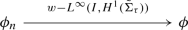
$$\begin{aligned} \phi\in & {} L^\infty (I, H^1({\tilde{\Sigma }}_\tau ))\\ \partial _\tau \phi\in & {} C^0(I, L^2({\tilde{\Sigma }}_\tau )) \end{aligned}$$As a consequence (this fact is proved in [24, p. 535]), we have:
$$\begin{aligned} \phi \in C^0(I, w-H^1({\tilde{\Sigma }}_\tau )). \end{aligned}$$In this context, on can prove the a priori estimates over the foliation \({\tilde{\Sigma }}_\tau \):
$$\begin{aligned} |E_\phi ({\tilde{\Sigma }}_\tau )-E_\phi ({\tilde{\Sigma }}_\mu )|\le C\left( \int _{[\tau ;\mu ]}E_\phi ({\tilde{\Sigma }}_r)\text {d}r\right) \end{aligned}$$The energy is then locally Lipschitz continuous. As a consequence, since \(\phi \) is in \(C^0(I, w-H^1({\tilde{\Sigma }}_\tau ))\), \(\phi \) is also in \(C^0(I, H^1({\tilde{\Sigma }}_\tau ))\).
- (a)
\(\square \)
4 Estimates for the characteristic Cauchy problem
In the previous section, it has been proved that the Cauchy problem admits a local solution to the characteristic Cauchy problem, relying only on the existence of a priori estimates for the solutions. The uniqueness has, so far, not be proved yet, as well as the continuity in the initial data. This can be achieved in various ways. The path we chose to follow is based on the work of Baez–Segal–Zhou [2] and relies on an a priori existence result of solutions to the Cauchy problem, which has been handled in a specific way separately in Sect. 3. The estimates are established by relying on a reduction to the Cauchy problem.
The setting is both the framework introduced by Hörmander and Baez–Segal–Zhou. The geometric setting and notations are the same as in the previous section, see Fig. 1, and the proof of Theorem 3.2.
Remark 4.1
The setting introduced by Hörmander considers only space-times of the form \(X\times {\mathbb {R}}\), where X is a compact manifold, a priori without boundary. The result can nonetheless be immediately extended to the case when the manifold X has a boundary. This can be seen using the following remark: the energy space remains \(H^1(X)\) (and not \({\dot{H}}{}^1(X)\)). Assume that the manifold with boundary \({\overline{X}}\) is embedded in a bigger compact manifold without boundary (which can always be done). If the boundary of X is at least \(C^1\), the space \(H^1(X)\) extends continuously into \(H^1({\overline{X}})\). As a consequence, all energy estimates involving \({\overline{X}}\) can be brought back onto X. In this specific case, the boundary of \(\Sigma _T\) is the intersection of \(\Sigma _T\) with \(J^-(p)\) and is, as a consequence, smooth.
One introduces first the following operator:
which associates with initial data \((\phi , \psi )\) the trace over \(C_{T}\) of the solution of the linear wave equation with initial data \((\phi , \psi )\) on \(\Sigma _T\). Following Hörmander [12], this operator has the following properties:
Theorem 4.2
(Hörmander) The linear operator \({\mathfrak {T}}\) is one-one, onto and bi-continuous, that is to say that there exists a constant C depending only on the geometry of the manifold such that, for all \((\phi , \psi )\) in \(H^1(\Sigma _0)\times L^2(\Sigma _0)\):
and
We introduce the extension operator \(E_{C}\) and \(E_{\Sigma _0}\), as considered in [29, Chapter V, Theorems 5 and 5’]:
These operators are continuous, and their norms depend solely on the curvature of the boundaries of C and \(\Sigma _0\) in \({\tilde{C}}\), and \({\tilde{\Sigma }}_0\), respectively.
We consider the remark of Baez et al. [2, Proof of Theorems 13 and 16]:
Lemma 4.3
Let \(\delta _0\) be an initial data set in \(H^1(C_T)\). Let H be a function defined over the foliation \((\Sigma _t)_t\) in \(C^1([0, T], L^2(\Sigma _t))\cap C^0([0, T], H^1(\Sigma _t))\). Then, the solution \(\delta \) of the Cauchy problem
can be extended to the past of \({\tilde{\Sigma }}_T\) by solving the Cauchy problem on \({\tilde{\Sigma }}_0\) with initial data \(E_{\Sigma _0}\left( {\mathfrak {T}}^{-1}(\delta _0)\right) \) for the equation:
where the function H is extended by 0 outside \(J^-(C_T)\).
For such an equation, the energy estimates are simple to obtain, since the foliation of reference to establish them have non-vanishing volume. For the sake of consistency, these estimates are nonetheless proved here. To that end, we introduce the stress-energy tensor
The energy of a function \(\phi \) on any weakly spacelike hypersurface S is defined as
where \(\star \) is the Hodge dual with respect to the metric g. In particular, one checks that
Lemma 4.4
Let \(\delta \) be as in Lemma 4.3. There exists an increasing function \(C: {\mathbb {R}}^+\rightarrow {\mathbb {R}}^+\) such that:
and
Proof
Since the techniques under considerations are standard, the proof is only sketched. The error term associated with the considered stress-energy tensor is
Applying Stokes theorem between \(\Sigma _0\) and \(\Sigma _s\), one gets immediately the following inequality:
One deals with the nonlinear term using Sobolev embeddings over the compact foliation \(\Sigma _\tau \), whose volume of leaves does not go to 0:
One finally gets
and using Grönwall’s inequality closes the estimates. \(\square \)
Let now be \(\theta \) and \(\xi \) be two functions in \(H^1(C_T)\) and consider the two characteristic Cauchy problems:
The function \(\delta \) defined as being the difference between u and v satisfies the wave equation
where
Using Lemma 4.3, we extend \(\delta \) to the whole cylinder by considering \(\delta \) to the problem
with initial data \(E_{\Sigma _{0}}\left( {\mathfrak {T}}^{-1}(\theta -\xi )\right) \). Using the continuity of trace operator, the continuity of the extension operator, and Lemma 4.4, one proves:
Proposition 4.5
There exists an increasing function C such that the following inequalities hold:
Proof
The proof of these energy inequalities is a direct consequence of Proposition 4.4. It suffices to notice that, for \(H^2=\phi ^2 +\phi \psi + \psi ^2\), using the triangular inequality,
Using a priori estimates such as the one proved in [14, Proposition 6.2], the later terms can be bounded by either
\(\square \)
Finally, an important consequence of the energy estimate (4.5) and Theorem 3.2 is the following proposition:
Proposition 4.6
The characteristic Cauchy problem:
admits at most one solution up to time T in \(C^0([0, T],H^1(\Sigma _t))\cap C^1([0,T], L^2(\Sigma _t))\).
5 Solving the characteristic Cauchy problem in the neighbourhood of \(i^0\)
5.1 Preliminary result
The purpose of this section is to explain how the characteristic Cauchy problem can be solved in the neighbourhood of the spacelike infinity \(i^0\) of the asymptotically simple manifold. The neighbourhood of \(i^0\) is assumed to be isometric to the Schwarzschild space-time to agree with the work of the Corvino–Schoen and Chruściel–Delay.
The Schwarzschild metric is given, in the standard spherical coordinates
Performing the change of coordinates
the metric takes the form
A conformal rescaling with a conformal factor \(\Omega =\frac{1}{R}\) is finally performed to define the unphysical metric:
Consider the domain \(\Omega ^+_{u_0} = \{u\le u_0\}\), for some \(u_0\) to be chosen later. It has been proved [14, 18] that the following lemma holds:
Lemma 5.1
Let \(\epsilon >0\). There exists \(u_0<0\), \(|u_0|\) large enough, such that the following decay estimates in the coordinate \((u,r,\theta , \psi )\) hold:
Furthermore, the vector field
is uniformly timelike in the region \(\Omega ^+_{u_0}\).

Neighbourhood of \(i^0\)
The parameter \(\epsilon \) will be chosen later when we perform the energy estimates. We define, in \(\Omega ^+_{u_0}=\{t>0, u<u_0\}\), the following hypersurfaces, for \(u_0\) given in \({\mathbb {R}}\) (Fig. 2):
\(S_{u_0}=\{u=u_0\}\), a null hypersurface transverse to \({{\mathscr {I}}}^+\);
\(\Sigma _{0}^{u_0>}=\Sigma _0\cap \{u_0>u\}\), the part of the initial data surface \(\Sigma _0\) in the past of \(S_{u_0}\);
\({{\mathscr {I}}}_{u_0}^+=\Omega ^+_{u_0}\cap {{\mathscr {I}}}^+\), the part of \({{\mathscr {I}}}^+\) beyond \(S_{u_0}\);
\({\mathcal {H}}_s=\Omega ^+_{u_0}\cap \{u=-sr^*\}\), for s in [0, 1], a foliation of \(\Omega ^+_{u_0}\) by spacelike hypersurfaces accumulating on \({{\mathscr {I}}}\).
The volume form associated with g in the coordinates \((R,u,\omega _{{\mathbb {S}}^2})\) is then:
If \(\phi \) is function defined on \(\Omega ^+_{u_0}\), one defines the following energies, in the domain \(\Omega _{u_0}^+\):
Proposition 5.2
([14, Proposition A.2]) There exists \(u_0\), such that the following energy estimates holds on \({\mathcal {H}}_s\) in \(\Omega ^+_{u_0}\), for all s in [0, 1]:
Furthermore, if one introduces the parameter
the following energy estimates holds:
Energy decay:
$$\begin{aligned} E_{\phi }({\mathcal {H}}_s) \lesssim E_{\phi }({\Sigma _0^{u_0<}}) \end{aligned}$$A priori estimates:
$$\begin{aligned} E({{\mathscr {I}}}^+_{u_0})+\int _{{{\mathscr {I}}}^+_{u_0}}\phi ^4\text {d}\mu _{{{\mathscr {I}}}^+}+E(S_{u_0})+ \int _{S_{u_0}}\phi ^4\text {d}\mu _{S_u} \approx E({\Sigma _0^{u_0<}}) + \int _{{\Sigma _0^{u_0<}}} u^4 \text {d}_{{\Sigma _0^{u_0<}}} \end{aligned}$$
5.2 Local existence for the Characteristic Cauchy problem on \({{\mathscr {I}}}^+\)
The purpose of this section is to prove that the Cauchy problem:
where \(H^{1}(S_{u_0})\) is defined as being the completion of the space of traces of smooth functions on \(S_{u_0}\) for the norm
\(T_{\text {lin}\,ab}\) being the stress-energy tensor associated with the linear wave equation. In a previous work [14], the following result has been proved:
using the fact that the leaves of the foliation \({\mathcal {H}}_s\) endowed with its induced metric are uniformly equivalent to a cylinder, it is possible to establish energy estimates for the difference of solutions of the nonlinear equation;
it is possible to establish an existence result for solutions of the nonlinear equation for small data, using either a Picard iteration (as in [13]) or Hörmander slowing down process.
Proposition 5.3
Let \(\phi \) and \(\psi \) be two solutions of the characteristic Cauchy problem and denote by \(\delta = \phi -\psi \) their difference. One denotes the energy of \(\delta \) by
where \(T_{\text {lin}\,ab}\) is the stress-energy tensor for \(\delta \) associated with the linear wave equation. Then, \(\delta \) satisfies the following energy estimates on the foliation \({\mathcal {H}}_s\);
In particular, the Cauchy problem (4.3) admits at most one solution in \(C^0([0,\epsilon ], H^1({\mathcal {H}}_s))\cap C^1([0,\epsilon ], L^2({\mathcal {H}}_s))\) and the energy
is continuous.
Proof
Let \(\phi \) and \(\psi \) be two global solutions of (4.3). Their difference \(\delta =\phi -\psi \) satisfies the equation:
Using the Stokes theorem between \({{\mathscr {I}}}^+_{u_0}\), \(S_{u_0}\) and \({\mathcal {H}}_s\), one gets, since \(\delta \) vanishes on \(S_{u_0}\) and \({{\mathscr {I}}}^+_{u_0}\):
As already said, Sobolev estimates can be performed uniformly on the foliation \(({\mathcal {H}}_s)\). As a consequence, using Hölder’s inequality, one gets:
where \(T^a\) is the approximate Morawetz vector field
The constant depends only on the \(L^\infty \)-bound of the scalar curvature. Finally, using Grönwall lemma, one gets that
As a consequence, the mapping
is continuous. Furthermore, the Cauchy problem (4.3) admits at most one unique solution in \(C^0([0,\epsilon ], H^1({\mathcal {H}}_s))\cap C^1([0,\epsilon ], L^2({\mathcal {H}}_s))\). \(\square \)
Proposition 5.4
Let \(\varepsilon \) be a positive real number. Then, for \(\varepsilon \) small enough depending on \(\theta \), the characteristic Cauchy problem (4.3) admits a unique solution in the neighbourhood of \({{\mathscr {I}}}^+_{u_0}\)
Proof
The proof relies on a fixed point argument. Consider \(\psi \) in \(C^0\left( [0,\epsilon ], H^1({\mathcal {H}}_s) \right) \). Let \(\phi \) be the solution of the Cauchy problem
This defines a mapping
One proves, using standard energy estimates that, for \(s\le \epsilon \),
In particular, \(\phi \) belongs to \(C^0\left( [0,\epsilon ], H^1({\mathcal {H}}_s) \right) \).
Let R be a positive real number. Assume that
Then, there exists an \(\epsilon \) small enough, depending on R, such that, for all \(\psi \) such that
then,
Furthermore, let \(\psi , {{\tilde{\psi }}}\) be two functions in \(C^0\left( [0,\epsilon ], H^1({\mathcal {H}}_s) \right) \), and consider \(\phi , {{\tilde{\phi }}}\) the corresponding solution to the problem (4.6). Their difference \(\phi -{{\tilde{\phi }}}\) satisfies
One easily proves, as in Proposition 5.3, that
where C is an increasing function of R. Hence, R fixed, for \(\epsilon \) small enough, the mapping \(\phi \mapsto \psi \) is a contraction of the ball of radius R in \(C^0\left( [0,\epsilon ], H^1({\mathcal {H}}_s) \right) \) endowed with the \(L^\infty _s H^1({\mathcal {H}}_s)\)-norm. The standard fixed point theorem provides the result. \(\square \)
6 Global Cauchy problem on \({{\mathscr {I}}}^+\)
The existence of global solutions to the Cauchy problem is proved using a gluing process: the Cauchy problem with data in \(H^1({{\mathscr {I}}}^+)\) is constructed up to a spacelike hypersurface and, then, considering the traces of the solution on two given hypersurfaces in the neighbourhood of \(i^0\) solved up to the initial time slice \(\Sigma _0\). The main issue arising in this process is that the constants arising in the energy estimates depend on the \(L^\infty \)-bounds of the metric and its inverse on the bounded neighbourhood of \(i^0\). Since the compactification we are working with has the particularity to have an asymptotic end at \(i^0\), these constants are not bounded on the whole future of \(\Sigma _0\). This problem is avoided as follows (see Fig. 3):
Let \(u_0\) be in \({\mathbb {R}}\) such as in Proposition 5.2.
Let \(\Sigma \) be a given spacelike hypersurface such that:
\(\Sigma \) is transverse to \({{\mathscr {I}}}^+\);
\(\Sigma \) is in the past of \(S_{u_0}\) and in the future of \(\Sigma _{0}\); in particular, \(\Sigma \) coincides with \(\Sigma _{0}\) far from \(i^0\).
These choices of \(u_0\) and \(\Sigma \) are made once for all.

Choosing \(\Sigma \)
Proposition 6.1
The characteristic Cauchy problem
admits a unique global solution in \({C^0([0,1], H^1({{\tilde{\Sigma }}}_s)) \cap C^1([0,1],L^2({{\tilde{\Sigma }}}_s))}\) where \(({{\tilde{\Sigma }}}_s)_{s>0}\) is a smooth spacelike foliation extending the definition of the foliation \(({\mathcal {H}}_s)\) in the neighbourhood of \(i_0\). Furthermore, if \({{\tilde{\phi }}}\) is another solution with initial data \({{\tilde{\theta }}}\), the following energy estimates holds: there exists a increasing function f such that
Proof
The proof of the theorem relies on the consecutive use of Theorem 3.2, Proposition 4.6 and of Proposition 5.4.
Let \(\theta \) be in \(H^1({{\mathscr {I}}}^+)\). Using Theorem 3.2, one proves that the Cauchy problem admits a solution \(\phi \) up to \(\Sigma \), as defined earlier. Then, using Proposition 5.4, there exists a \(\epsilon >0\) such that the Cauchy problem given by
exists in
Consider the time slice \({\mathcal {H}}_\epsilon \). This time slice can be extended into \({{\hat{M}}}\) into a spacelike Cauchy slice denoted by \({\mathcal {H}}\). The timelike vector field T is extended as a timelike vector to \({\mathcal {H}}\). One now considers the functions \((\psi _0,\psi _1)\) defined piecewise by:
and
By construction, since \({\mathcal {H}}\) is a spacelike Cauchy surface on the unphysical space-time, the result from Cagnac–Choquet-Bruhat [3] can be applied immediately to prove the existence of a unique solution to the Cauchy problem with data \((\psi _0, \psi _1)\) on \({\mathcal {H}}\) up to the Cauchy surface \(\Sigma _0\). Furthermore, this solution belongs to \({C^0([0,1], H^1({{\tilde{\Sigma }}}_s)) \cap C^1([0,1],L^2({{\tilde{\Sigma }}}_s))}\).
Consequently, there exists a global solution of the Cauchy problem:
obtained by gluing the solutions of the Cauchy problems obtained in Theorem 3.2 and Proposition 5.4. \(\square \)
7 Existence and regularity of the scattering operator
The purpose of this section is to prove the regularity and the existence of conformal scattering operator for the nonlinear wave equation
In the context of asymptotically simple space-times with regular \(i^\pm \), such as the one considered in [14, 18], it has been proved by Mason and Nicolas, for the scalar wave equation, that the trace operators
can be obtained from the inverse wave operators \({{\tilde{\Omega }}}^\pm \) as follows: let \(F_\pm \) be the null geodesic flows identifying the hypersurface \(\Sigma _0\) with \({{\mathscr {I}}}^\pm \); then, \({\mathfrak {T}}^\pm \) are given by
where \(F^\star \) is the pullback by the null geodesic flows \(F_\pm \). The same result will hold in the context of the nonlinear equation. The conformal scattering result which is stated here should consequently be considered as a standard scattering result for a non-stationary metric for a nonlinear wave equation. The existence of scattering operators was obtained on the flat background for sub-critical wave equations by [10, 11, 15, 32, 33].
One considers the operators
defined by
where u is the unique solution of the Cauchy problem on the conformally compactified space-time
One finally introduces the conformal scattering operator defined as
Theorem 7.1
The operators \({\mathfrak {T}}^\pm : H^1(\Sigma _0)\times L^2(\Sigma _0) \rightarrow H^1({{\mathscr {I}}}^\pm )\) are well-defined, invertible and locally bi-Lipschitz, that is to say that \({\mathfrak {T}}^\pm \) and \(({\mathfrak {T}}^\pm )^{-1}\) are Lipschitz on any ball in \(H^1(\Sigma _0)\times L^2(\Sigma _0) \) and \(H^1({{\mathscr {I}}}^\pm )\), respectively.
Proof
The existence and continuity of the operators guarantee the existence of solution to the Cauchy problem for the conformal wave equation, see Proposition 2.2. The existence of their inverses and their continuity are obtained thanks to the Lipschitzness guaranteed by the energy estimate of Proposition 6.1. \(\square \)
The final product of this paper, the existence of a scattering operator, is achieved by composing the operator \(({\mathfrak {T}}^{-})^{-1}\) with \({\mathfrak {T}}^{+}\):
Corollary 7.2
There exists a locally bi-Lipschitz invertible operator \({\mathfrak {S}} : H^{1}(\Sigma ) \times L^{2}(\Sigma ) \rightarrow H^1({{\mathscr {I}}}^\pm ) \). This operator generalises the notion of classical scattering operators (defined when the metric is static) to non-stationary metrics.
Proof
As mentioned before, the construction of \({\mathfrak {S}} \) is a straightforward consequence of Theorem 7.1. The fact that the operator coincides with the classical notion of scattering operator is stated in [18]. \(\square \)
Notes
By geometric equation, we would like to insist that the operator defining the equation is depending on the metric.
References
Andersson, L., Chruściel, P.T.: On hyperboloidal Cauchy data for vacuum Einstein equations and obstructions to smoothness of Scri. Commun. Math. Phys. 161(3), 533–568 (1994)
Baez, J.C., Segal, I.E., Zhou, Z.-F.: The global Goursat problem and scattering for nonlinear wave equations. J. Funct. Anal. 93(2), 239–269 (1990). https://doi.org/10.1016/0022-1236(90)90128-8
Cagnac, F., Choquet-Bruhat, Y.: Solution globale d’une équation non linéaire sur une variété hyperbolique. J. Math. Pures Appl. (9) 63(4), 377–390 (1984)
Christodoulou, D.: The global initial value problem in general relativity. In: Gurzadyan, V.G., Jantzen, R.T., Ruffini, R. (eds.) Proceedings of the Ninth Marcel Grossmann Meeting on General Relativity, vol. Part A, pp. 44–54 (2000)
Chruściel, P.T., Delay, E.: Erratum: Existence of non-trivial, vacuum, asymptotically simple spacetimes. Class. Quantum Gravity 19(12), 3389 (2002). https://doi.org/10.1088/0264-9381/19/12/501
Chruściel, P.T., Delay, E.: Existence of non-trivial, vacuum, asymptotically simple spacetimes. Class. Quantum Gravity 19(9), L71–L79 (2002). https://doi.org/10.1088/0264-d9381/19/9/101
Corvino, J., Schoen, R.M.: On the asymptotics for the vacuum Einstein constraint equations. J. Differ. Geom. 73(2), 185–217 (2006)
Frauendiener, J.: Conformal Infinity. Living Rev. Relativ. 3(1), 4 (2000). https://doi.org/10.12942/lrr-2000-4
Friedlander, F.G.: Radiation fields and hyperbolic scattering theory. Math. Proc. Camb. Philos. Soc. 88(3), 483–515 (1980). https://doi.org/10.1017/S0305004100057819
Hidano, K.: Nonlinear small data scattering for the wave equation in \({ R}^{4+1}\). J. Math. Soc. Jpn. 50(2), 253–292 (1998). https://doi.org/10.2969/jmsj/05020253
Hidano, K.: Conformal conservation law, time decay and scattering for nonlinear wave equations. J. Anal. Math. 91, 269–295 (2003). https://doi.org/10.1007/BF02788791
Hörmander, L.: A remark on the characteristic Cauchy problem. J. Funct. Anal. 93(2), 270–277 (1990). https://doi.org/10.1016/0022-1236(90)90129-9
Joudioux, J.: Characteristic Cauchy problem and conformal scattering in general relativity. Theses, Université de Bretagne occidentale - Brest (2010)
Joudioux, J.: Conformal scattering for a nonlinear wave equation. J. Hyperbolic Differ. Equ. 9(1), 1–65 (2012). https://doi.org/10.1142/S0219891612500014
Karageorgis, P., Tsutaya, K.: Small-data scattering for nonlinear waves of critical decay in two space dimensions. Differ. Integral Equ. 19(6), 601–626 (2006)
Lions, J.-L., Magenes, E.: Non-homogeneous boundary value problems and applications, vol. I. Translated from the French by P. Kenneth, Die Grundlehren der mathematischen Wissenschaften, Band 181. Springer, New York, p. xvi+357 (1972)
Lions, J.-L.: Dérivées intermédiaires et espaces intermédiaires. C. R. Acad. Sci. Paris 256, 4343–4345 (1963)
Mason, L.J., Nicolas, J.-P.: Conformal scattering and the Goursat problem. J. Hyperbolic Differ. Equ. 1(2), 197–233 (2004). https://doi.org/10.1142/S0219891604000123
Mason, L.J., Nicolas, J.-P.: Regularity at space-like and null infinity. J. Inst. Math. Jussieu 8(1), 179–208 (2009). https://doi.org/10.1017/S1474748008000297
Mason, L.J., Nicolas, J.-P.: Peeling of Dirac and Maxwell fields on a Schwarzschild background. J. Geom. Phys. 62(4), 867–889 (2012). https://doi.org/10.1016/j.geomphys.2012.01.005
Mokdad, M.: Maxwell field on the Reissner–Nordström–De Sitter manifold: decay and conformal scattering. Theses, Université de Bretagne occidentale - Brest (2016)
Mokdad, M.: Conformal Scattering of Maxwell fields on Reissner–Nordström–de Sitter black hole spacetimes. Ann. Inst. Fourier 69(9), 2291–2329 (2019). http://aif.cedram.org/item?id=AIF_2019__69_5_2291_0
Mokdad, M.: Decay of Maxwell Fields on Reissner–Nordström–de Sitter Black Holes (2017). arXiv e-prints , arXiv:1704.06441 [math.AP]
Nicolas, J.-P.: On Lars Hörmander’s remark on the characteristic Cauchy problem. Ann. Inst. Fourier (Grenoble) 56(3), 517–543 (2006)
Nicolas, J.-P., Pham, T.X.: Peeling on Kerr spacetime: linear and semi-linear scalar fields. Ann. Henri Poincaré 20(10), 3419–3470 (2019). https://doi.org/10.1007/s00023-019-00832-0
Penrose, R., Rindler, W.: Spinors and Space-Time. Spinor and Twistor Methods in Space-Time Geometry, Vol. 1 and 2. Cambridge Monographs on Mathematical Physics. Cambridge University Press, Cambridge (1988)
Pham, T.X.: Peeling and conformal scattering on the spacetimes of the general relativity. Theses, Université de Bretagne occidentale - Brest (2017)
Sogge, C.D.: Lectures on Non-Linear Wave Equations, 2nd edn. International Press, Boston (2008). pp. x+205
Stein, E.M.: Singular Integrals and Differentiability Properties of Functions. Princeton Mathematical Series, No. 30. Princeton University Press, Princeton (1970)
Taujanskas, G.: Conformal scattering of the Maxwell-scalar field system on de Sitter space (2018). arXiv e-prints arXiv:1809.01559 [math.AP]
Taylor, M.E.: Partial Differential Equations. I. Applied Mathematical Sciences: Basic Theory, vol. 115. Springer, New York (1996). https://doi.org/10.1007/978-1-4684-9320-7
Tsutaya, K.: Scattering theory for semilinear wave equations with small data in two space dimensions. Proc. Jpn. Acad. Ser. A Math. Sci. 68(8), 227–231 (1992)
Tsutaya, K.: Scattering theory for semilinear wave equations with small data in two space dimensions. Trans. Am. Math. Soc. 342(2), 595–618 (1994). https://doi.org/10.2307/2154643
Acknowledgements
Open access funding provided by Projekt DEAL. I want to thank Jean-Philippe Nicolas, whose strong incentive incited me to complete these notes which I drafted a long time ago. The referees have contributed a lot to the improvement of this note, and I would like to thank them for their comments.
Author information
Authors and Affiliations
Corresponding author
Additional information
Publisher's Note
Springer Nature remains neutral with regard to jurisdictional claims in published maps and institutional affiliations.
Appendix A: A trace theorem
Appendix A: A trace theorem
One of the critical points of the proof of the existence theorem 2.2 is a trace theorem, which has already been used in [24, p. 19, proof of Theorem 4.3]. Most of the material presented here can be found in [31, Section 4.3, p. 281 sqq.] for the interpolation and in [16, Theorems 2.3 and 3.1] for the continuity of trace operators. Finally, it is important to note that the essential ideas and proofs of this appendix are contained in [16, Chapter 3, Section 8.2]. The purpose of this appendix is also to give further understanding and details on the work of Hörmander on the Cauchy problem [12] and clarify some points contained in [24].
Let X and Y be two Hilbert spaces such that
X is continuously embedded in Y;
X is dense in Y.
The interpolation spaces between X and Y are denoted by
Let a, b be two elements in \({\mathbb {R}}\cup \{\pm \infty \}\) and m be an positive integer. One considers the following space:
The following trace theorem then holds, see [16, theorems 2.3 and 3.1, chapter 1,]:
Theorem A.1
(Lions–Magenes) Let \(\phi \) be in W(a, b). Then, for all j in \(\{0,\dots ,m-1 \}\), the derivatives of \(\phi \) satisfy:
\(\frac{\partial ^j \phi }{\partial t^j}\) is in \(L^2([a,b];[X,Y]_{\frac{j}{m}})\);
\(\frac{\partial ^j \phi }{\partial t^j}\) is in \(C^0_b([a,b];[X,Y]_{\frac{j+1/2}{m}})\).
Remark A.2
The theory developed by Lions and Magenes applies to general Hilbert spaces, independently of the geometric context (in particular, if one works on a space with boundary or on a compact manifold).
One applies this result to the following situation: let M be a compact manifold and consider
\(X= H^1(M)\);
\(Y = H^{-1}(M)\).
The interpolation spaces between both are given by [31, Section 4.3, Proposition 3.1]:
Let a, b be in \({\mathbb {R}}\) and \(m=2\). Applying Theorem A.1 then gives: if u satisfies:
then:
\(\frac{\partial \phi }{\partial t}\) is in \(L^2([a,b],L^2(M))\) (\(\theta = \frac{1}{2}\));
\(\phi \in C^0([a,b],L^2(M))\);
\(\frac{\partial u}{\partial t}\) is in \(C^0([a,b],H^{-\frac{1}{2}}(M))\) (\(\theta = \frac{3}{4}\)).
Remark A.3
Obtaining that the derivative is actually in \(C^0([a,b],H^{0}(M))\) would require
To improve this result, one notices the following:
Lemma A.4
Let \(I=[a,b]\) be a time interval and \(s<\sigma \) be two real numbers and consider a function \(\phi \) such that
Then, \(\phi \) belongs to \(C^0(I,H^s (M)-w)\).
Remark A.5
This is a particular case of [16, Chapter 3, Lemma 8.1].
Proof
Let \(\phi \) be in \(H^s(M)\) such as in the proposition and consider w in \(H^\sigma (M)\). One considers the function
Let \(t_0\) be in I. The purpose is to prove that f is continuous in \(t_0\).
Let \((w_k)\) be a sequence of smooth function converging towards w in \(H^s\). Let \(\epsilon \) be a positive real and consider:
Since, using Cauchy–Schwarz inequality,
and since \((w_k)\) converges towards w in \(H^s\), and since \(\phi \) is in \(L^\infty (I,H^s(M))\), there exists a K such that:
One now considers the interpolation operators between \(L^2(M)\) and \(H^s(M)\) (for arbitrary s):
This is a family of unbounded, self-adjoint operators for which:
Since \(w_K\) is smooth, it admits a pre-image by \({\mathfrak {F}}^{-1}_s\circ {\mathfrak {F}}_\sigma \). As a consequence, one has:
Cauchy–Schwarz inequality implies then:
Since \(\phi \) is in \(C^0(I,H^\sigma (M))\), there exists an open neighbourhood U of \(t_0\) in I such that, for all t in \(U\subset I\):
As a consequence, for all t in U,
that is to say that f is continuous in \(t_0\). \(\square \)
One now considers a model case fitting the context of the wave equation. Let \((I \times M, -N^2 \text {d}t^2+g_t)\) be a Lorentzian manifold, I being a compact interval. One defines the energy of the function as being the function of t and \(\phi \) in \(H^1(M)\) and \(\psi \) in \(L^2(M)\) by:
The final lemma required to achieve the wanted regularity for the solution of the characteristic Cauchy problem for the wave equation is the following:
Lemma A.6
One assumes that, for all \((\phi , \psi )\) in \(H^1(M)\times L^2(M)\), the function:
is continuously differentiable in I. Let \(\phi \) be a function such that:
\(\phi \) is in \(C^0(I,H^1(M)-w)\); as a consequence, \(\phi \) lies in \(L^\infty (I,H^1(M))\)
\(\partial _t \phi \) is in \(C^0(I,L^2(M)-w)\); as a consequence, \(\phi \) lies in \(L^\infty (I,L^2(M))\).
The function:
is furthermore assumed to be continuous in t.
Then, \(\phi \) and \(\partial _t \phi \) are in fact in \(C^0(I,H^1(M))\) and \(C^0(I,L^2(M))\).
Proof
The proof of this fact can be found in [16, Chapter 3, Section 8.4, p. 279]. For the sake of self-consistency, the proof is quoted here, with some adaptations to our framework.
Let t be in I and consider \((t_n)_n\) a sequence of elements of I converging towards t and define the quantity:
Since \(\phi \) is in \(C^0(I,H^1(M)-w)\) and \(\partial _t \phi \) is in \(C^0(I,L^2(M)-w)\), the last two terms converge towards \(-2E(t, \phi (t),\partial _t\phi (t))\). Since the energy is assumed to be continuous, the first tow terms converge towards \(2E(t, \phi (t),\partial _t\phi (t))\).
The sequence \((\xi _n)\) converges then towards 0 when n grows. As a consequence, \(\phi \) and \(\partial _t\phi \) are in \(C^0(I,H^1(M))\) and \(C^0(I,L^2(M))\), respectively. \(\square \)
Rights and permissions
Open Access This article is licensed under a Creative Commons Attribution 4.0 International License, which permits use, sharing, adaptation, distribution and reproduction in any medium or format, as long as you give appropriate credit to the original author(s) and the source, provide a link to the Creative Commons licence, and indicate if changes were made. The images or other third party material in this article are included in the article’s Creative Commons licence, unless indicated otherwise in a credit line to the material. If material is not included in the article’s Creative Commons licence and your intended use is not permitted by statutory regulation or exceeds the permitted use, you will need to obtain permission directly from the copyright holder. To view a copy of this licence, visit http://creativecommons.org/licenses/by/4.0/.
About this article

Cite this article
Joudioux, J. Hörmander’s method for the characteristic Cauchy problem and conformal scattering for a nonlinear wave equation. Lett Math Phys 110, 1391–1423 (2020). https://doi.org/10.1007/s11005-020-01266-0
Received:
Revised:
Accepted:
Published:
Issue Date:
DOI: https://doi.org/10.1007/s11005-020-01266-0