Development of Multi-GPU–Based Smoothed Particle Hydrodynamics Code for Nuclear Thermal Hydraulics and Safety: Potential and Challenges

Park, So-Hyun; Jo, Young Beom; Ahn, Yelyn; Choi, Hae Yoon; Choi, Tae Soo; Park, Su-San; Yoo, Hee Sang; Kim, Jin Woo; Kim, Eung Soo

doi:10.3389/fenrg.2020.00086

ORIGINAL RESEARCH article

Front. Energy Res., 05 June 2020
Sec. Nuclear Energy
Volume 8 - 2020 | https://doi.org/10.3389/fenrg.2020.00086

Development of Multi-GPU–Based Smoothed Particle Hydrodynamics Code for Nuclear Thermal Hydraulics and Safety: Potential and Challenges

So-Hyun Park

Young Beom Jo

Yelyn Ahn

Hae Yoon Choi

Tae Soo Choi

Su-San Park

Hee Sang Yoo

Jin Woo Kim

Eung Soo Kim^*

Department of Nuclear Engineering, Seoul National University, Seoul, South Korea

Advanced modeling and analysis are always essential for the development of safe and reliable nuclear systems. Traditionally, the numerical analysis codes used for nuclear thermal hydraulics and safety are mostly based on mesh-based (or grid-based) methods, which are very mature for well-defined and fixed domains, both mathematically and numerically. In support of their robustness and efficiency, they have been well-fit into many nuclear applications for the last several decades. However, the recent nuclear safety issues encountered in natural disasters and severe accidents are associated with much more complex physical/chemical phenomena, and they are frequently accompanied by highly non-linear deformations. Sometimes, this means that the conventional methods encounter many difficult technical challenges. In this sense, the recent advancement in the Lagrangian-based CFD method shows great potential as a good alternative. This paper summarizes recent activities in the development of the SOPHIA code using Smoothed Particle Hydrodynamics (SPH), a well-known Lagrangian numerical method. This code incorporates the basic conservation equations (mass, momentum, and energy) and various physical models, including heat transfer, turbulence, multi-phase flow, surface tension, diffusion, etc. Additionally, the code newly formulates density and continuity equations in terms of a normalized density in order to handle multi-phase, multi-component, and multi-resolution problems. The code is parallelized using multiple graphical process units (GPUs) through multi-threading and multi-streaming in order to reduce the high computational cost. In the course of the optimization of the algorithm, the computational performance is improved drastically, allowing large-scale simulations. For demonstration of its applicability, this study performs three benchmark simulations related to nuclear safety: (1) water jet breakup of FCI, (2) LMR core melt sloshing, and (3) bubble lift force. The simulation results are compared with the experimental data, both qualitatively and quantitatively, and they show good agreement. Besides its potential, some technical challenges of the method are also summarized for further improvement.

Introduction

Since the Fukushima accident, nuclear safety issues related to severe accidents [i.e., Fuel–Coolant Interaction (FCI), In-Vessel Melt Retention (IVMR), and Molten Corium Concrete Interaction (MCCI)] (Bauer et al., 1990; Sehgal et al., 1999; Ma et al., 2016; Bonnet et al., 2017) and natural disasters (i.e., tsunami, earthquake, etc.; Zhao et al., 1996; Barto, 2014) are gaining more attention than ever. These issues generally involve various physically/chemically complicated phenomena such as fluid dynamics, heat transfer, multiple phases, multiple components, diffusion, fluid–solid interaction, chemical reaction, phase change, etc., successively interacting each other. For example, when the molten core relocates to the lower head of the vessel, the hot fuel melt contacts with water coolant followed by FCI. This phenomenon includes hydraulic fragmentation, heat transfer, phase change, multi-phase flow, etc., which have the potential to trigger a steam explosion or porous debris bed formation (Allelein et al., 1999; Sehgal et al., 1999). This accident progression adds complexities to the phenomenon, such as solidification and vapor bubble dynamics. In the IVMR situation, a huge corium pool is formed at the lower head of the vessel, and it is continuously cooled by external vessel coolant. In this case, the corium pool experiences numerous observed phenomena, such as natural convection with strong turbulence, crust formation, stratification, ablation, and eutectic and focusing effects (Ma et al., 2016). In the MCCI, more complicated phenomena occur through intricate interactions between the molten fuel, concrete, and water (Bonnet et al., 2017). In such scenarios, the reactor vessel and/or containment integrity is threatened in various ways, such as by steam explosion, thermal/chemical ablation, direct impinging, and so on. In addition to the above examples, the large complexity of the physics/chemistry involved in these phenomena still leaves us with significant uncertainty in understanding and predicting reactor safety.

In recent years, advances in Computational Fluid Dynamics (CFD) have provided an opportunity to explore the nuclear thermal hydraulics and safety in more a realistic and mechanistic manner. The mesh-based numerical methods [i.e., Finite Difference Method (FDM), Finite Element Method (FEM), and Finite Volume Method (FVM)] have a long development history in many engineering fields, including nuclear engineering, and they are highly matured both mathematically and numerically. Based on their robustness and efficiency, they have dominated the CFD field for decades, and they are successfully applied in various applications. Generally, the mesh-based methods are known to be suitable for handling a pre-defined computational domain where the boundaries and interfaces are not moving. However, they suffer from difficulties in handling complex phenomena accompanied by highly non-linear deformations, which are frequently encountered in recent nuclear safety-related problems such as multi-phase flow, a free surface, and large deformation.

In order to address and handle the weaknesses of the mesh-based methods, several new methods have been proposed and developed based on a Lagrangian meshless framework (Liu and Liu, 2003; i.e., SPH, MPS, MPM, DEM, etc.). Those methods are advantageous in handling free surface flow, interfacial flow, and large deformation because the mesh or mass points are carried with the flow, possessing the properties of the material. Additionally, the interfaces or boundaries are traced naturally in the process of simulation. In this study, Smoothed Particle Hydrodynamics (SPH), which is the most widely used meshless CFD method, has been selected and used for various applications (Wang et al., 2016). The SPH method discretizes the fluid system into a set of particles (or parcels) that contain the material properties, and these particles move according to the governing equations. The most widely used SPH method is the Weakly Compressible SPH (WCSPH) method, which allows slight compressibility, even for liquid fluids, using an equation of state (EOS). In this method, the basic conservation equations such as for mass, momentum, and energy conservation are solved with various physical models of heat transfer, turbulence, multi-phase flow, phase change, diffusion, etc. (Jo et al., 2019). Many recent studies showed that the SPH methodology has very good potential for handling complicated phenomena in nuclear engineering and other engineering fields (Wang et al., 2016; Park et al., 2018; Jo et al., 2019).

Although many successful studies on the SPH have been reported, the SPH methodology has high computational cost, like other particle-based methods, for many reasons. In this regard, the SPH method suffers from the limitation of the simulation time and size (Valdez-Balderas et al., 2013; Nishiura et al., 2015; Guo et al., 2018). Therefore, enhancing its computational performance efficiently and effectively is essential to make this method more practical and useful. Recently, massive parallel-computer-system-based techniques have been actively employed to address this issue, such as the multi-core Central Processing Unit (CPU), Graphics Processing Unit (GPU), and Many Integrated Core (MIC) processor (Nishiura et al., 2015). Such techniques demonstrate high computational performance by executing computations in parallel. In particular, the GPU, which was originally designed for graphical data processing, is increasingly being used in parallel computing in general engineering and science because of the efficiency arising by having thousands of computing cores. These general-purpose GPUs (GPGPU) are generally suitable for high-throughput computations featuring data-parallelism. Therefore, GPU-based parallelization is strongly advocated for and preferred in the SPH method, which consists of highly linear numerical expressions that can be computed independently one by one (Valdez-Balderas et al., 2013).

The SOPHIA code is an SPH-based numerical code developed by Seoul National University (SNU) for conducting simulations of nuclear thermal hydraulics and safety (Jo et al., 2019). The original SOPHIA code was written in C++ and parallelized using a single GPU. The main physics behind this code includes (1) liquid flow, (2) heat transfer, (3) melting/solidification, (4) natural convection, (5) multi-phase flow, etc. In this study, the physical models and numerical methods of the SOPHIA code have been highly improved in order to simulate the phenomena accurately. Moreover, the code has been parallelized using multiple GPUs to obtain high-resolution and large-scale simulations for more practical applications. This parallelization has been implemented through multi-threading and multi-streaming. The multi-threading technique divides the computational domain into GPUs and then executes the GPUs concurrently. The multi-streaming technique effectively schedules computing tasks within each GPU. Based on these techniques, the SOPHIA code has achieved a drastic improvement in computational performance. To demonstrate its capability and applicability, this study performs simulations on three different benchmark experiments related to nuclear safety: (1) water jet breakup of FCI, (2) Liquid Metal Reactor (LMR) core sloshing, and (3) bubble lift force. The simulation results are then compared with experimental data, both qualitatively and quantitatively.

This paper summarizes the overall features of the newly developed SOPHIA code, including its governing equations, algorithms, and parallelization methods, along with benchmark simulations. Section Smoothed Particle Hydrodynamics (SPH) describes the basic SPH concepts and the physical models implemented in the code. Section Code Implementation explains the parallelization techniques used for multiple GPU computation. Section Benchmark Analysis presents three benchmark simulations with some validations. Section Summary and Conclusion summarizes and concludes this study.

Smoothed Particle Hydrodynamics (SPH)

Smoothed Particle Hydrodynamics (SPH) is a computational method used for simulating the mechanics of continuum media based on a Lagrangian meshless framework. It was first developed by Gingold and Monaghan (1977) and Lucy (1977) for astrophysics. In recent years, it has been extended to many other research fields such as mechanical engineering, ocean engineering, chemical engineering, and nuclear engineering. Since SPH is a mesh-free method, it is ideal for simulating phenomena dominated by complicated boundary dynamics like free surface flows or with large boundary deformations. In addition, this method simplifies the model implementation and parallelization. This section briefly summarizes the basic concepts of SPH and how the basic conservation laws and physical models are constructed for nuclear thermal-hydraulics and safety applications.

Fundamentals of SPH

Mathematically, SPH approximation is based on the theory of integral interpolants using a delta function.

\begin{array}{l} f (r) = \int_{Ω} f (r^{'}) δ (r - r^{'}) d r^{'} & (1) \end{array}

where the variable r denotes the point vector in infinite volume domain Ω, and δ denotes the Dirac delta function, which has a value of zero everywhere except for at a certain point, and whose integral over the entire region is equal to one. Although Equation (1) is mathematically valid, it is numerically difficult to handle due to the discontinuity of the delta function. Therefore, the basic idea of SPH is to approximate the Dirac delta function using a continuous kernel function and discretize the integral by summation (Monaghan, 1992).

\begin{array}{l} f (r_{i}) = \sum_{j} \frac{m_{j}}{ρ_{j}} f (r_{j}) W (r_{i} - r_{j}, h) & (2) \end{array}

where m and ρ denote the particle mass and particle density. The subscripts i and j denote center particle and neighboring particle, respectively. W(r_i − r_j, h) stands for the kernel function, where h denotes the influencing area of the kernel weighting function. The kernel function is a symmetric weighting function of particle distance that should be normalized over its support domain. The particle system and conditions for kernel function are described in Figure 1. This kernel determines the weight of a certain particle at r_j with regard to the distance from the center (r_i) (Liu and Liu, 2003). Table 1 summarizes the kernel functions that are commonly used. This study applied the Wendland C2 kernel (Dehnen and Aly, 2012), which helps to maintain low numerical instability.

FIGURE 1

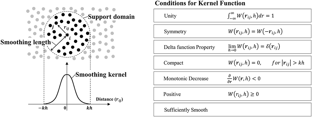
Figure 1. Schematic diagram of SPH kernel approximation.

TABLE 1

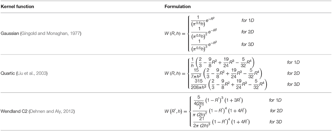
Table 1. Commonly used SPH kernel functions $(R = \frac{| {r - r}^{'} |}{h}, R^{*} = \frac{| {r - r}^{'} |}{2 h})$ .

Spatial derivatives of a function can also be simply approximated in a similar way by taking derivatives of a kernel function as follows (Monaghan, 1992).

\begin{array}{l} \nabla f (r_{i}) = \sum_{j} V_{j} f (r_{j}) \nabla W (r_{i} - r_{j}, h) & (3) \end{array}

\begin{array}{l} \nabla \cdot f (r_{i}) = \sum_{j} V_{j} f (r_{j}) \nabla \cdot W (r_{i} - r_{j}, h) & (4) \end{array}

\begin{array}{l} \nabla^{2} f (r_{i}) = \sum_{j} V_{j} f (r_{j}) \nabla^{2} W (r_{i} - r_{j}, h) & (5) \end{array}

where $V_{j} = \frac{m_{j}}{ρ_{j}}$ denotes the particle volume. When the particles are distributed uniformly in space, the SPH approximations of scalar function and its derivatives ensure the second-order accuracy (Liu and Liu, 2003). However, an irregular particle distribution or truncation near the free surface causes numerical errors (Belytschko et al., 1996). Such particle-domain-induced problems, referred to as particle inconsistency, influence the accuracy of the simulation profoundly. In order to restore the particle inconsistency and improve the accuracy, various methods have been proposed. For the scalar approximation, applying a Shepard filter is the most well-known method to restore the particle inconsistency (Randles and Libersky, 1996).

\begin{array}{l} f (r_{i}) = \frac{\sum_{j} f (r_{j}) W (r_{i} - r_{j}, h) V_{j}}{\sum_{j} W (r_{i} - r_{j}, h) V_{j}} & (6) \end{array}

This Shepard filter normalizes the kernel to correct the under-estimated contributions of particle deficiency. For the derivative approximation, the following Kernel Gradient Correction (KGC) is commonly applied (Bonet and Lok, 1999).

\begin{array}{l} \nabla f (r_{i}) = \sum_{j} f (r_{j}) L_{i} \nabla W (r_{i} - r_{j}, h) V_{j} & (7) \end{array}

\begin{array}{l} L_{i} \\ = {[\begin{array}{l} \sum_{j} (x_{j} - x_{i}) W_{x} V_{j} \sum_{j} (y_{j} - y_{i}) W_{x} V_{j} \sum_{j} (z_{j} - z_{i}) W_{x} V_{j} \\ \sum_{j} (x_{j} - x_{i}) W_{y} V_{j} \sum_{j} (y_{j} - y_{i}) W_{y} V_{j} \sum_{j} (z_{j} - z_{i}) W_{y} V_{j} \\ \sum_{j} (x_{j} - x_{i}) W_{z} V_{j} \sum_{j} (y_{j} - y_{i}) W_{z} V_{j} \sum_{j} (z_{j} - z_{i}) W_{z} V_{j} \end{array}]}^{- 1} & (8) \end{array}

where [W_x, W_y, W_z] = ∇W. This KGC filter is incorporated into the original kernel derivative to re-evaluate the contributions of irregularly distributed particles. Other than the above correction methods, more sophisticated kernel approximation schemes for SPH have been proposed by several researchers. They include the Corrective Smoothed Particle Method (CSPM), Finite Particle Method (FPM), and Kernel Gradient Free (KGF). They all aim to resolve the particle inconsistency caused by particle truncation at the boundaries as well as irregular particle distribution. The details can be found in the Bonet and Lok (1999), Chen and Beraun (2000), Liu and Liu (2006), and Huang et al. (2016).

Governing Equations of the SOPHIA Code

The SOPHIA code consists of three basic conservation laws (mass, momentum, and energy conservations), which are expressed as follows in a Lagrangian manner.

\begin{array}{l} Continuity Equation : \frac{d ρ}{d t} = - ρ \nabla \cdot u & (9) \end{array}

\begin{array}{l} Navier - Stokes Equation : \frac{d u}{d t} = - \frac{\nabla p}{ρ} + ν \nabla^{2} u + g \\ + f_{e x t} & (10) \end{array}

\begin{array}{l} 1 st Law of Thermodynamics : \frac{d h}{d t} = - \frac{λ}{ρ} \nabla^{2} T + \overset{∙}{q} & (11) \end{array}

where u, p, ν, g, f_ext, h, λ, T, and $\overset{∙}{q}$ denote the velocity vector, pressure, kinematic viscosity, gravitational acceleration, external body force, specific enthalpy, thermal conductivity, temperature, and heat generation rate, respectively. In the SOPHIA code, these equations are formulated in SPH as described in section Fundamentals of SPH.

Continuity Equation (Mass Conservation)

The SOPHIA code is based on the conventional weakly compressible SPH (WCSPH) (Gingold and Monaghan, 1977; Lucy, 1977; Monaghan, 1992), which allows slight compressibility for liquid according to the given equation of state (EOS). Therefore, the density estimation is very important for predicting pressure in the fluid flow. The SOPHIA code estimates the density by either direct mass summation or a continuity equation (Monaghan, 1992). In the direct mass summation, the density is estimated by the following SPH kernel approximation.

\begin{array}{l} ρ_{i} = \sum_{j} m_{j} W (r_{i} - r_{j}, h) & (12) \end{array}

Although Equation (12) is the most commonly used formulation in the WCSPH, it frequently suffers from an over-smoothing problem for the density near an interface or a large-density-gradient field, which is easily encountered in multi-component/multi-fluid/multi-phase flows. In this case, the over-smoothed density becomes the main source of numerical error/instability by generating unphysical pressure force near the interface (Hu and Adams, 2006). To avoid this issue, the SOPHIA code adapts the newly proposed formulation, which is derived based on the normalized density as follows (Park et al., 2019).

\begin{array}{l} \frac{ρ_{i}}{ρ_{r e f, i}} = \sum_{j} \frac{m_{j}}{ρ_{j}} (\frac{ρ_{j}}{ρ_{r e f, j}}) W_{i j} & (13) \end{array}

where ρ_ref denotes the reference density of the particle and W_ij = W(r_i − r_j, h). Numerically, this new equation can eliminate the density smoothing problem without any numerical treatments or additional issues. As mentioned above, the density of the fluid can also be evaluated by solving a continuity equation. The continuity equation in the SOPHIA code is expressed as follows.

\begin{array}{l} {(\frac{d ρ}{d t})}_{i} = - ρ_{i} \sum_{j} \frac{m_{j}}{ρ_{j}} (u_{i} - u_{j}) \cdot \nabla_{i} W_{i j} \\ + ξ h c_{0} \sum_{j} \frac{m_{j}}{ρ_{j}} ψ_{i j} \cdot \nabla_{i} W_{i j} & (14) \end{array}

where ξ, c₀ denote the diffusion intensity coefficient, speed of sound and $\nabla_{i} W_{i j} = \frac{\partial W (r_{i} - r_{j}, h)}{\partial r_{i}}$ . In this formulation, an artificial density diffusion term (the last term on the RHS), which is called δ-SPH, is added to remove high-frequency numerical pressure noise (Molteni and Colagrossi, 2009). The diffusion coefficient in Equation (14) is recommended to be set as (0 < ξ ≤ 0.2). Determination of the variable ψ_ij is proposed by several studies. In the SOPHIA code, the method proposed by Antuono et al. (2010) is used, as follows.

\begin{array}{l} ψ_{i j} = 2 (ρ_{i} - ρ_{j}) \frac{r_{i j}}{| r_{i j} |} \\ - [\sum_{j} V_{j} (ρ_{j} - ρ_{i}) L_{i} \nabla_{i} W_{i j} + \sum_{k} V_{k} (ρ_{k} - ρ_{j}) L_{j} \nabla_{j} W_{j k}] & (15) \end{array}

where L denotes KGC kernel correction as mentioned in section Fundamentals of SPH. The subscripts j and k denote the neighboring particle of particle i (main particle) and the neighboring particle of particle j (neighbor of the main particle), respectively. The continuity equation can also be re-formulated in terms of the normalized density as in the direct mass summation (Park et al., 2019).

\begin{array}{l} {(\frac{d ρ}{d t})}_{i} = - ρ_{i} \sum_{j} \frac{m_{j}}{ρ_{j}} u_{i j} \cdot \nabla_{i} W_{i j} + {(\frac{ρ}{ρ_{r e f}})}_{i} {(\frac{d ρ_{r e f}}{d t})}_{i} \\ + ξ h c_{0} \sum_{j} \frac{m_{j}}{ρ_{j}} ψ_{n d, i j} \cdot \nabla_{i} W_{i j} & (16) \end{array}

\begin{array}{l} ψ_{n d, i j} = 2 ρ_{r e f, i} (\frac{ρ_{i}}{ρ_{r e f, i}} - \frac{ρ_{j}}{ρ_{r e f, j}}) \frac{r_{i j}}{| r_{i j} |} \\ - [{ρ_{r e f, i} \nabla (\frac{ρ}{ρ_{r e f}})}_{i}^{L} + {ρ_{r e f, j} \nabla (\frac{ρ}{ρ_{r e f}})}_{j}^{L}] & (17) \end{array}

\begin{array}{l} {ρ_{r e f, i} \nabla (\frac{ρ}{ρ_{r e f}})}_{i}^{L} \\ = ρ_{r e f, i} \sum_{j} V_{j} (\frac{ρ_{j}}{ρ_{r e f, j}} - \frac{ρ_{i}}{ρ_{r e f, i}}) L_{i} \nabla_{i} W_{i j} & (18) \end{array}

where u_ij = u_i − u_j and the variable ψ_nd,ij denotes a normalized-density formulated diffusion term. Equation (16) consists of a mass transport term, a reference density time derivative term (derived only from mass variation), and a density diffusive term. The mass transport term is equivalent to the original continuity equation. The time derivative term can be explicitly calculated by the chain rule. The normalized δ-SPH term diffuses out the numerical noise of the normalized density $(\frac{ρ}{ρ_{r e f}})$ , while the original model diffuses out the density itself. This normalized continuity equation can achieve the same improvement as the new mass summation (Equation 13). These newly devised equations (Equations 13, 16) estimate the density ratio that would be applied in EOS, thus addressing the density-smoothing problem. In the case of a uniform density field, these formulations exactly converge to the conventional SPH density equations.

Navier-Stokes Equation (Momentum Conservation)

The momentum conservation (Equation 10) can be decomposed into several individual terms: pressure force, viscous force, gravitational force, and external force. The following is the basic SPH form of the momentum equation used in the SOPHIA code.

\begin{array}{l} {(\frac{d u}{d t})}_{i} = - \sum_{j} m_{j} \frac{(p_{i} + p_{i})}{ρ_{i} ρ_{j}} \nabla_{i} W_{i j} \\ + \sum_{j} \frac{4 m_{j}}{ρ_{i} ρ_{j}} \frac{μ_{i} μ_{j}}{(μ_{i} + μ_{j})} u_{i j} \frac{r_{i j}}{| r_{i j} |^{2}} \cdot \nabla W_{i j} + g + f_{e x t} & (19) \end{array}

where μ denotes the viscosity involving laminar and turbulence effects, and u_ij = u_i − u_j. As mentioned in many SPH studies (Monaghan, 1992, 1994; Liu and Liu, 2003; Wang et al., 2016), there are various different ways to convert mathematical equations into SPH formulations.

Table 2 summarizes the SPH-formulated models for pressure force and laminar viscous force. The pressure force model (Equation 20), first proposed by Monaghan (1992), was derived from the Euler-Lagrangian equations. This pairwise symmetric model ensures the linear momentum conservation inherently, but it calculates an unphysical pressure gradient at the interfaces of different fluids (density) like multi-phase flow. To handle the discontinuity of multi-phase flow, a new pressure force model (Equation 21) was suggested by Liu and Liu (2003). This equation not only satisfies pairwise symmetricity but also estimates the pressure gradient based on the particle volume so that physically valid pressure forces are obtained for the discontinuous density field. However, near the free surface, where the particle pressure generally oscillates around zero, the negative pressure causes this model to calculate an unphysical repulsive force, which leads to numerical instability. To address this issue, the minus-signed model (Equation 22) was proposed by Sun et al. (2017). This pressure force model eliminates the unphysical force near the free surface, but it should only be applied to the particles close to the free surface. Laminar viscous force models have also been developed in a similar manner to pressure force models. Particularly, the viscous force models vary in their way of treating viscosity. At the interfaces where the particle viscosities are different such as in multi-phase or multi-fluids, both Equations (23) and (25) employ a harmonic mean, while Equation (24) employs an arithmetic mean value. On the other hand, all the viscous models are valid for a discontinuous density field, because they calculate the force based on the particle volume. Finally, Equation (19) is selected to be well-suited for multi-phase/multi-fluid flow simulations.

TABLE 2

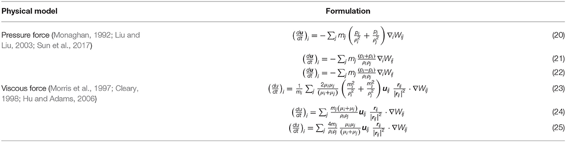
Table 2. Pressure and viscous force models.

1st Law of Thermodynamics (Energy Conservation)

For non-radiative, homogeneous, and isotropic energy conservation, heat transfer is mainly subject to conduction and convection. In a Lagrangian framework, the convective heat transfer can be resolved inherently, and therefore energy conservation is simply expressed by the following (Monaghan, 2005).

\begin{array}{l} {(\frac{d h}{d t})}_{i} = \sum_{j} \frac{4 m_{j}}{ρ_{i} ρ_{j}} (\frac{λ_{i} λ_{j}}{λ_{i} + λ_{j}}) (T_{i} - T_{j}) \frac{r_{i j}}{| r_{i j} |^{2}} \cdot \nabla W_{i j} + {\overset{∙}{q}}_{i} & (26) \end{array}

where h, λ, T, and $\overset{∙}{q}$ denote the specific enthalpy, thermal conductivity, temperature, and heat source, respectively. The heat source or heat flux of boundary conditions is represented as the source term of energy conservation. In the SPH method, these source terms are modeled as a specific heat rate, and they are exerted on the particles that are involved.

Equation of State

In the WCSPH, the pressure of the fluid is evaluated by an equation of state (EOS). The most commonly used EOS is Tait's equation (Monaghan, 1994). In the SOPHIA code, the modified form is implemented in terms of reference density as follows.

\begin{array}{l} p_{i} = \frac{{c_{0}}^{2} ρ_{r e f, i}}{γ} [{(\frac{ρ_{i}}{ρ_{r e f, i}})}^{γ} - 1] & (27) \end{array}

where c₀, ρ_ref, and γ denote the speed of sound, reference density, and EOS stiffness parameter, respectively; γ is recommended to be set as (1 ≤ γ ≤ 7). This equation calculates the pressure based on the density ratio between the particle density and the reference density, which allows a slight volume compression for liquid fluids.

Turbulence

As in the conventional CFD methods, the turbulence models in the SPH are divided into two groups: (1) Reynolds Average Navier-Stokes (RANS)-based models and (2) Large Eddy Simulation (LES)-based models. In the SOPHIA code, both models are implemented. In the case of a RANS-based k-ϵ model (Violeau and Issa, 2007), the viscous force of the fluid flow is calculated by considering both laminar and turbulence viscous effects as follows.

\begin{array}{l} {(\frac{d u}{d t})}_{i}^{t u r b} = \sum_{j} \frac{m_{j}}{ρ_{i} ρ_{j}} \frac{4 μ_{e, i} μ_{e, j}}{(μ_{e, i} + μ_{e, j})} u_{i j} \frac{r_{i j} \cdot \nabla W_{i j}}{| r_{i j} |^{2}} & (28) \end{array}

\begin{array}{l} μ_{e} = μ_{v} + μ_{T}, μ_{T} = \frac{ρ C_{μ} k^{2}}{ϵ} & (29) \end{array}

where μ_v, μ_T, C_μ, k, and ϵ denote laminar viscosity (material property), turbulent viscosity, turbulent viscous coefficient, turbulence kinetic energy, and turbulent dissipation rate, respectively. The turbulence kinetic energy and the dissipation rate are estimated by solving transport equations. The transport equation for the turbulence kinetic energy is expressed by

\begin{array}{l} {(\frac{d k}{d t})}_{i} = P_{i} - ϵ_{i} + \sum_{j} \frac{m_{j}}{ρ_{i} ρ_{j}} (μ_{k, i} + μ_{k, j}) k_{i j} \frac{r_{i j} \cdot \nabla W_{i j}}{| r_{i j} |^{2}} & (30) \end{array}

\begin{array}{l} μ_{k} = μ_{v} + \frac{μ_{T}}{σ_{k}} & (31) \end{array}

where k_ij = k_i − k_j and σ_k = 1.0. The RHS of the above equation consists of turbulence production (P), turbulence dissipation (ϵ), and turbulence diffusion terms. The production of turbulence kinetic energy is calculated by the strain tensor of the time-averaged velocity, and the dissipation rate is calculated by solving the transport equation as follows.

\begin{array}{l} {(\frac{d ϵ}{d t})}_{i} = \frac{ϵ_{i}}{k_{i}} (C_{ϵ, 1} P_{i} - C_{ϵ, 2} ϵ_{i}) \\ + \sum_{j} \frac{m_{j}}{ρ_{i} ρ_{j}} (μ_{ϵ, i} + μ_{ϵ, j}) ϵ_{i j} \frac{r_{i j} \cdot \nabla W_{i j}}{| r_{i j} |^{2}} & (32) \end{array}

\begin{array}{l} μ_{ϵ} = μ_{v} + \frac{μ_{T}}{σ_{ϵ}} & (33) \end{array}

where C_{ϵ, 1} and C_{ϵ, 2} denote the constant coefficients and σ_ϵ = 1.3. The Sub-Particle Scale (SPS) turbulence model, based on LES, is commonly employed in the SPH simulations (Rogers and Dalrymple, 2008). The Smagorinsky model, the basis of the SPS model, formulates the eddy viscosity as the product of the characteristic length scale and the strain rate tensor, which is defined by time-averaged velocity. In the SPH formulation, the SPS model is expressed as follows (Rogers and Dalrymple, 2008; Zhang et al., 2017).

\begin{array}{l} ν_{S P S} = {(C_{s} l)}^{2} | S^{α β} | & (34) \end{array}

\begin{array}{l} S^{α β} = \frac{1}{2} [\sum_{j} \frac{m_{j}}{ρ_{j}} (u_{j}^{α} - u_{i}^{α}) \frac{\partial W_{i j}}{\partial r_{i}^{β}} \\ + \sum_{j} \frac{m_{j}}{ρ_{j}} (u_{j}^{β} - u_{i}^{β}) \frac{\partial W_{i j}}{\partial r_{i}^{α}}] & (35) \end{array}

where l and C_s denote the particle spacing and the pre-defined coefficient. S^αβ denotes the strain rate tensor in the Einstein notation (α, β = 1, 2, 3) and $| S^{α β} | = \sqrt{2 S : S}$ . In this model, the smallest turbulence scale is modeled as a sub-particle-scale stress tensor that includes the interactions at all scales (resolved scale, unresolved scale, and cross-scale). The turbulence viscous force of the SPS model is added to the momentum equation.

\begin{array}{l} {(\frac{d u}{d t})}_{i}^{t u r b} = \sum_{j} m_{j} (\frac{τ_{i}^{α β}}{ρ_{i}^{2}} + \frac{τ_{j}^{α β}}{ρ_{j}^{2}}) \cdot \nabla W_{i j} & (36) \end{array}

\begin{array}{l} τ^{α β} = ρ (2 ν_{T} S^{α β} - \frac{2}{3} S^{r r} δ^{α β}) - \frac{2}{3} ρ C_{I} Δ l^{2} δ^{α β} & (37) \end{array}

where τ^αβ and δ^αβ denote the sub-particle scale stress tensor and the Kronecker delta in the Einstein notation, respectively (α, β, γ = 1, 2, 3).

Molecular Diffusion

In the SOPHIA code, the molecular diffusion of the chemical components is formulated similarly to the heat transfer model (Monaghan, 2005).

\begin{array}{l} {(\frac{d S}{d t})}_{i} = \sum_{j} \frac{4 m_{j}}{ρ_{i} ρ_{j}} (\frac{D_{i} D_{j}}{D_{i} + D_{j}}) (S_{i} - S_{j}) \frac{r_{i j} \cdot \nabla W_{i j}}{| r_{i j} |^{2}} & (38) \end{array}

where D and S denote the molecular diffusivity and molecular concentration, respectively. It is noted that the above equation is based on the molecular concentration, and if the other definition for concentration is used, the diffusivity should be incorporated within it. When binary diffusion (material A and B) is involved, the reference density time derivative term ${(\frac{d ρ_{r e f}}{d t})}_{i}$ in the continuity equation (Equation 16) can be expressed as follows using molar fraction (Park et al., 2019).

\begin{array}{l} {(\frac{d ρ_{r e f}}{d t})}_{i} = χ_{i} \sum_{j} \frac{m_{j}}{ρ_{i} ρ_{j}} [\frac{{4 D}_{i} D_{j}}{D_{i} + D_{j}}] x_{i j} \nabla_{i} W_{i j} & (39) \end{array}

\begin{array}{l} χ_{i} = ρ_{r e f, i}^{2} (\frac{1}{ρ_{A}} - \frac{1}{ρ_{B}}) (\frac{M_{A} M_{B}}{{(x M_{A} + (1 - x) M_{B})}^{2}}) & (40) \end{array}

where M and x denote the molar mass and molar fraction. The coefficient χ describes the conversion from a molar fraction (Δx) to a mass fraction.

Buoyancy Force

Buoyancy force is considered in the SOPHIA code in two ways: (1) a Boussinesq model, and (2) a Non-Boussinesq model. The Boussinesq model is the most commonly used in the conventional SPH simulations. It assumes a slight density variation (Δρ≪ρ) of the fluid, which ensures that the density has a negligible effect on the main flow (Boussinesq approximation). Therefore, it is straightforward to apply the model by adding the following buoyancy force term to the momentum equation (Equation 19).

\begin{array}{l} {(\frac{d u}{d t})}_{i}^{f b} = (1 - α_{T} (T - T_{0})) g & (41) \end{array}

where fb, α_T, and T₀ denote the buoyancy force, thermal expansion coefficient, and reference temperature, respectively. This Boussinesq model is simple to apply, and the results are relatively good. However, the model reliability is significantly reduced when the density variation is spatially large. For a large density gradient, a non-Boussinesq model, which is applicable for SPH, has been developed and adopted for the SOPHIA code (Park et al., 2019). In this model, the density change is directly estimated by mass and volume changes of particles, which are determined by temperature and concentration as follows.

\begin{array}{l} m_{i} = m_{0, i} (1 + α_{S} (S - S_{0})) & (42) \end{array}

\begin{array}{l} V_{i} = V_{0, i} {(1 - α_{T} (T_{i} - T_{0}))}^{- 1} & (43) \end{array}

\begin{array}{l} ρ_{r e f, i} = \frac{m_{i}}{V_{i}} & (44) \end{array}

where α_T, α_S, T₀, and S₀ denote thermal expansion coefficient, saline contraction coefficient, initial temperature, and initial concentration, respectively. m₀ and V₀ denote the initial particle mass and initial particle volume, respectively. In this model, the mass, volume, and reference density of the particles are updated in every time step. The resultant reference density is used in the pressure calculation of the EOS (Equation 27). This approach not only allows large density-gradient-driven flow beyond the Boussinesq approximation but also represents the real physics more properly.

Surface Tension

In the SOPHIA code, two types of surface tension models are employed: (1) a Continuum Surface Force (CSF) model, and (2) an Intermolecular Potential Force (IPF) model. The CSF model estimates the surface tension force at the macroscopic scale. In this model, the surface tension force is expressed as the product of the surface curvature and the surface normal (Brackbill et al., 1992). According the previous studies (Morris, 2000; Hu and Adams, 2006), there are several ways to determine the curvature and surface normal, and the SOPHIA code adopted the following forms.

\begin{array}{l} {(\frac{d u}{d t})}_{i}^{C S F} = - \frac{σ_{i}}{ρ_{i}} κ_{i} n_{i} & (45) \end{array}

\begin{array}{l} n_{i} = \sum_{j} \frac{1}{V_{i}} (V_{i}^{2} + V_{j}^{2}) c_{i j} \nabla W_{i j} & (46) \end{array}

\begin{array}{l} κ_{i} = - d \frac{\sum_{j} V_{j} (\hat{n_{i}} - φ_{i j} \hat{n_{j}}) \cdot \nabla W_{i j}}{\sum_{j} V_{j} | r_{i j} | | {\nabla W}_{i j} |} & (47) \end{array}

\begin{array}{l} c_{i j} = {\begin{matrix} \begin{matrix} 0 f o r f_{i} = f_{j} \\ \frac{ρ_{i}}{ρ_{i} + ρ_{j}} f o r f_{i} \neq f_{j} \end{matrix} \end{matrix}, φ_{i j} = {\begin{matrix} \begin{matrix} \begin{matrix} 1 f o r f_{i} = f_{j} \\ \begin{matrix} - 1 f o r f_{i} \neq f_{j} \end{matrix} \end{matrix} \end{matrix} \end{matrix} & (48) \end{array}

where σ, κ, n, and d denote a surface tension coefficient, the curvature, surface-normal vector, and dimension, respectively (d = 1, 2, 3). $\hat{n_{i}}$ denotes the unit surface-normal vector. The notation f_i = f_j means that the phase of the fluid particle “i” is the same as that of particle “j,” and f_i ≠ f_j means the opposite case.

In the IPF model (Tartakovsky and Meakin, 2005), the interaction between particle i and neighboring j is considered in terms of molecular dynamics, such as repulsive force for short range and attractive force for long range. The combination of these forces naturally determines the interfacial particle distance. Therefore, calculations of curvature and surface normal are not required. In addition, the wettability effect can be estimated straightforwardly. This model is applied to the momentum equation (Equation 19) as an additional particle interaction force.

\begin{array}{l} {(\frac{d u}{d t})}_{i}^{I P F} = - \frac{1}{m_{i}} \sum_{j} f_{i j} & (49) \end{array}

where f_ij denotes inter-particle force between particle i and its neighbor j. Many previous studies have developed various different forms of the inter-particle force. Table 3 summarizes some of them.

TABLE 3

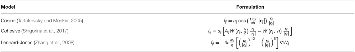
Table 3. Inter-particle force terms for the IPF surface tension model.

Multi-Phase Flow

Multi-phase phenomena are frequently encountered in nuclear thermal-hydraulics and safety issues. Since the SPH method is based on the Lagrangian framework, no surface detection or tracking method is necessary, which is essential for Eulerian-based CFD methods. Therefore, handling multi-phase flow with SPH is relatively simple and easy compared to the conventional Eulerian-based methods. The SOPHIA code has carefully adopted and organized the governing equations based on first principle in order to capture the multi-phase physics. Nevertheless, an additional term is introduced to stabilize the interface between the phases (Grenier et al., 2009). The interface sharpness force used in the SOPHIA code is formulated as follows.

\begin{array}{l} {(\frac{d u}{d t})}_{i}^{I S} = - \frac{ε}{m_{i}} \sum_{j} (| p_{i} | V_{i}^{2} + | p_{j} | V_{j}^{2}) \nabla W_{i j}, f o r f_{i} \neq f_{j} & (50) \end{array}

where ε is a tuning parameter that ranges between 0.01 and 0.1 (Grenier et al., 2009). The notation f_i ≠ f_j means that the phase of the fluid particle “i” is dissimilar to that of particle “j.” The kernel summation of the RHS only includes a neighboring particle ‘j’ that belongs to a different phase to particle “i.” This force should be large enough to stabilize the interface between the phases, but it should be small enough not to cause any unphysical effects.

Particle Shifting

As mentioned in section Fundamentals of SPH, particle deficiency and irregular distribution are the main sources of numerical errors in the SPH interpolations. Particle shifting is one of the methods to address this issue. It adjusts the particle position to enhance the uniformity of the distribution. The SOPHIA code adopted the shifting method proposed by Lind et al. (2012). This adjusts the particle spacing in proportion to the particle number density, which is an indicator of particle uniformity. In this method, the particle adjustment vector (δr) is evaluated by the following equation.

\begin{array}{l} δ r_{i} = - 0.5 h^{2} \sum_{j} V_{j} (1 + R {(\frac{W (r_{i j}, h)}{W (Δ r, h)})}^{n}) \nabla W_{i j} & (51) \end{array}

where R and n denote the constant parameters, set as to be 0.2 and 4, respectively. δr denotes the initial particle spacing. In every time step, the particle positions are updated by adding adjustment vector $(r_{i}^{*} = r_{i} + δ r_{i})$ . The particle properties on the new positions can be updated through SPH interpolation depending on the proposed numerical scheme.

Time Integration

In the SOPHIA code, a modified predictor-corrector scheme is applied (Gomez-Gesteira et al., 2012). The predictor-corrector scheme divides the time integration into two steps and determines the physical variables (position, velocity, density, and energy) and their time derivatives in turn. First, the prediction step extrapolates the physical variables as follows.

\begin{array}{l} {\begin{array}{l} u_{Δ t + \frac{Δ t}{2}}^{p} = u_{t} + \frac{Δ t}{2} {(\frac{d u}{d t})}_{t - \frac{Δ t}{2}} \\ r_{Δ t + \frac{Δ t}{2}}^{p} = r_{t} + \frac{Δ t}{2} {(\frac{d r}{d t})}_{t - \frac{Δ t}{2}} \\ ρ_{Δ t + \frac{Δ t}{2}}^{p} = ρ_{t} + \frac{Δ t}{2} {(\frac{d ρ}{d t})}_{t - \frac{Δ t}{2}} \end{array} & (52) \end{array}

where t and Δt denote time and time step, respectively. Superscript p denotes “predictor.” The time derivatives of position, velocity, density, and energy are newly evaluated by solving the discretized SPH governing equations based on the predicted values. After that, the field variables are re-integrated over the full time step using the updated time derivatives in the correction step.

\begin{array}{l} {\begin{array}{l} u_{Δ t + t}^{c} = u_{t} + Δ t {(\frac{d u}{d t})}_{t + \frac{Δ t}{2}} \\ r_{Δ t + t}^{c} = r_{t} + Δ t {(\frac{d r}{d t})}_{t + \frac{Δ t}{2}} \\ ρ_{Δ t + t}^{c} = ρ_{t} + Δ t {(\frac{d ρ}{d t})}_{t + \frac{Δ t}{2}} \end{array} & (53) \end{array}

where the superscript c denotes “corrector.” These corrected values become initial values for the next time step.

Code Implementation

The SPH generally has very high computational cost compared to conventional CFD methods. To address this issue, massive parallel-computer-system-based techniques have been actively employed in the SPH field, and the general-purpose GPU (GPGPU) is one of the most commonly favored. The GPU was originally developed for effective graphic rendering using thousands of parallel cores, but currently, its usage has been extended widely into general science and engineering applications due to the high-throughput computations and data-parallelism. Since the SPH formulations have no non-linear equations and every particle is calculated independently, the SPH code implementation is suitable for GPU parallelization.

In previous research by Jo et al. (2019), the SOPHIA code was fully parallelized using a single GPU, and it was demonstrated that the computational cost can be significantly reduced by GPU parallelization when compared to serial CPU computing. However, due to the limitation of the internal memory size of a single GPU, the allowable number of particles was highly restricted, being about 15 million particles for the original code. Therefore, it became essential to distribute computational load using multiple GPUs, which is critical for many practical large-scale applications. For this reason, the code has been restructured and fully parallelized using multiple GPUs along with domain decomposition. The technical details are summarized in the following sections.

GPU Implementation

Basic Algorithm

Figure 2 shows the basic algorithm of the code. The algorithm consists of several main steps and the sub-steps in the gray box in Figure 2. The gray box indicates that they are parallelized using multiple GPUs. The bold characters (Multi-GPU Allocation, Sub-domain Division, and Inter-GPU Communication) indicates the added steps for domain decomposition and data exchange between GPUs for distributing the computational load to multiple GPUs. The other steps are quite similar to the original SOPHIA code based on a single GPU (Jo et al., 2019). The first step of the code is Initialization. In this step, the input parameters and the initial particle information (position, velocity, temperature, pressure, property, etc.) are read from external input files and stored in the computer memory. This process is conducted by a single host CPU. After this process, the computational domain is divided into multiple sub-domains to distribute computational load and memory, and each GPU is assigned to each sub-domain, respectively. This allows the GPU to solve the governing equations and the physical models for only assigned/allocated sub-domain. Then, the particle data of the CPU host are copied to GPUs to have only their own sub-domains separately (Multi-GPU Allocation). The details are explained in section Multi-GPU Allocation. Once this process is completed, each GPU has the initial particle input data along with additional buffer data of the nearby domain for data exchange. The main loop is started from the Prediction step, which is conducted for predictor-corrector time integration, as explained in section Time Integration. After the Prediction step, the particle positions are updated, and the sub-domain is partitioned into four groups according to Sub-domain Division. This step is applied for optimizing the computational load and data transfer of the GPUs. According to the particle groups, calculation and data transfer are differently scheduled. The details are explained in section Sub-domain Division. Once this step is completed, neighboring particles are searched for every particle (NNPS). NNPS is the key step in the particle simulation since it usually entails the largest computational load. In this code, the uniform grid and sorting-based algorithm are implemented with full GPU adaptation. Once this process is done, each particle has its neighboring particle information, which is necessary for the following particle interaction steps. The NNPS algorithm implemented here is briefly explained in section Concurrent Execution. After the NNPS step, the particle interactions are calculated according to the SPH equations and physical models (density, momentum, energy, etc.) explained in section Smoothed Particle Hydrodynamics (SPH). For the SPH interpolations, massive parallel GPU mapping is applied extensively. The details can be found by reference to Jo et al. (2019). After the particle interactions, the corrector step in the time integration is followed, with major updates. Once all these main calculation steps are completed, it is checked whether the updated particles escape from the original subdomain. If so, their information is transferred to the new subdomain by memory copying to adjacent GPUs (Inter-GPU Communication). After this step is finished, all the GPUs have the newly updated particle data with a fully preserved computational domain. The simulation then proceeds to the next time step in a loop. This multi-GPU parallel algorithm consists of two-level parallelization. At the higher level, multiple GPUs concurrently execute the main loops within the decomposed sub-domains (Multi-GPU Concurrent Execution), and at the lower level, each GPU carries out parallel computation (mapping or sorting) and data transmission for each sub-domain using thousands of computing cores simultaneously.

FIGURE 2

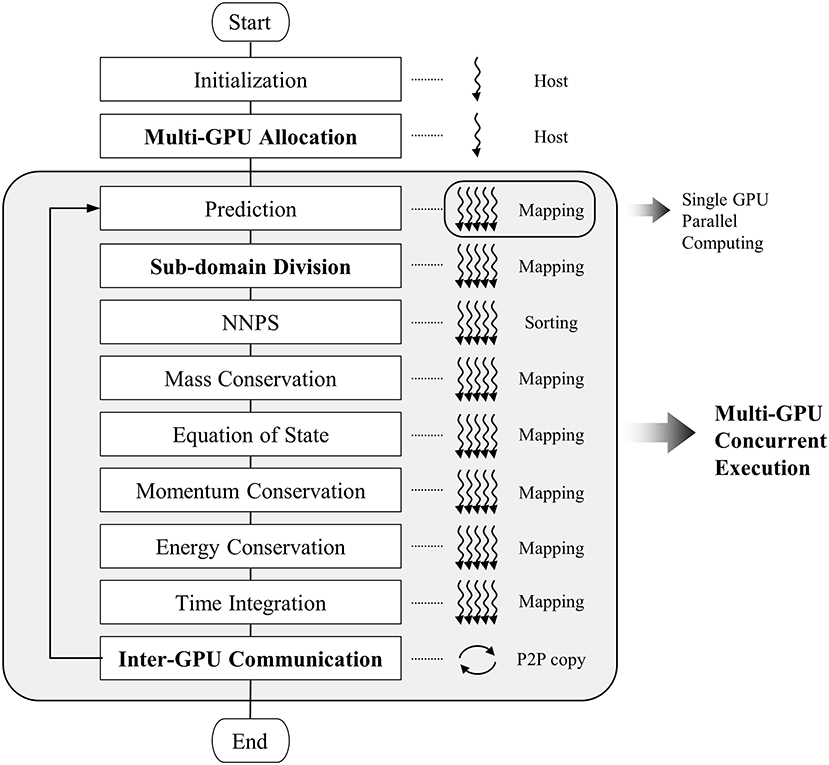
Figure 2. Algorithm of the SOPHIA code.

Multi-GPU Allocation

The multi-GPU allocation divides a whole computational domain into small sub-domains, as shown in Figure 3. First, as many threads are created as there are GPUs. The generated threads control the GPUs which are assigned the same index number, repectively. Then, the computational domain is divided in a specific direction (x, y, or z) to have a similar number of particles, and then the threads allocate these sub-domains to their own GPUs. Currently, the code allows the domain decomposition in only one direction, because it minimizes the memory usage for data exchange in the inter-GPU communication.

FIGURE 3

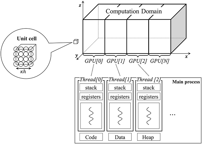
Figure 3. Schematic process of the multi-GPU allocation step.

Sub-domain Division

After the domain is decomposed and each sub-domain data is allocated to each GPU, the sub-domain is partitioned into four small sections for more efficient computation and data exchange. Figure 4 shows the concept of the sub-domain division. R0 is the inner particle region. The particles located in R0 have little chance to escape the sub-domain in a single time step. Therefore, the particle in this region is not involved in the data exchange. R1 is the outer particle region. The particles in R1 have some chance to escape the sub-domain boundary during time integration. Therefore, the particles in this region must be traced to determine whether they still exist in the sub-domain after position update. R2 is the outer buffer region. The particles in R2 are located on the right outside of the sub-domain boundary. Since this region is overlapped with the R1 of adjacent GPUs, the particles in this region are only involved in the calculation of the R1 particles. R3 is the dummy region. The particles in R3 are not involved in any computation and data exchange processes.

FIGURE 4

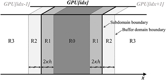
Figure 4. Concept of sub-domain division.

Concurrent Execution

After subdomains are partitioned, each GPU individually calculates the particle behaviors. As shown in Figure 2, the Nearest Neighbor Particle Search (NNPS) is proceeded with prior to the SPH interpolation steps. In the SPH, the NNPS step is the most time-consuming part; hence, the performance of the whole algorithm depends heavily on the efficiency of the NNPS. In the SOPHIA code, the NNPS is optimized using an algorithm based on a uniform grid and parallel sorting (Harada and Howes, 2011) that re-arranges the array of particles according to the order of each cell index. Figure 5 shows the concept of the NNPS algorithm with a uniform grid and sorting.

1. The computational domain is divided into the grid cells.

2. The cell index (CI) is calculated and assigned to every particle.

3. The particle array is sorted (PI^*) and ordered by cell index (CI^*).

4. The starting (Cstr) and ending (Cend) particle index arrays are constructed.

FIGURE 5

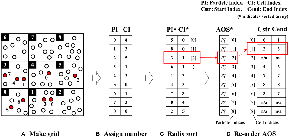
Figure 5. A demonstration of nearest-neighbor particle search by sorting. (A) Make grid, (B) assign number, (C) radix sort, and (D) re-order AOS.

The subsequent processes are performed during the SPH interpolation using these starting particle indices and ending particle indices. In the SPH interpolation, the particles in the adjacent cells are scanned and it is checked whether the distance from the center particle “i” is within the search range.

Once the NNPS step is complete, the density of each particle is calculated by solving either the mass summation or continuity equation. The particle pressure is then calculated according to the EOS. Afterward, all the particle interactions, including momentum conservation, energy conservation, molecular diffusion, etc., are computed with the physical models described in section Smoothed Particle Hydrodynamics (SPH). For all these calculations, parallel mapping is used. This method calls the same number of computing cores as there are particles, and each core computes the equations of each particle in parallel.

Inter-GPU Communication

After time integration and position update are conducted, the particles across the boundaries are checked, and information is exchanged between the adjacent GPUs through peer-to-peer (P2P) memory copy. Figure 6 shows the schematic process of the inter-GPU communication. First, the particles in R1 are labeled as “left” or “right” depending on their position, as shown in Figure 6A. The GPU[idx] sends the “left” particle data to the “idx-1”th GPU and the “right” data to the “idx+1”th GPU. Conversely, the “left” data of GPU[idx+1] and the “right” data of GPU[idx-1] are transferred to GPU[idx] and stored in memory. Among the received data, some particles may cross the boundaries and enter into the “idx”th subdomain. These particles remain as R1, and the rest are re-assigned as R2 to serve as neighbors of R1 particles. The unnecessary data will be dumped as dummy particles (R3) at the Sub-domain Division step of the next loop. This repetitive sub-domain division and inter-GPU communication ensures that each GPU occupies the subdomain that overlaps some buffer regions with the neighbor GPUs.

FIGURE 6

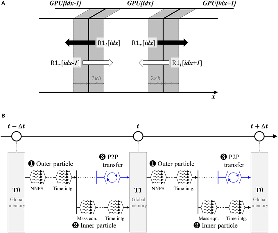
Figure 6. Schematic process of the inter-GPU communication step: (A) concept of inter-GPU communication and (B) multi-stream scheme with time marching.

In order to increase the efficiency of the inter-GPU communication, multi-streaming is applied in the code. The basic concept is shown in Figure 6B. In this algorithm, the calculations are split into two parallel streams. In one stream, the particle interactions of the physical models are solved. At the same time, Peer-to-Peer (P2P) memory transfer is conducted in the other stream in parallel. A combination of two streams reduces latency time effectively since data copying (referring to P2P copy) and kernel execution (referring to particle calculation) do not share computing resources. In addition, the data transaction is reliably completed during the calculation because the number of inner particles is much larger than that of outer particles.

Evaluation of Multi-GPU Parallel Performance

In the previous research, it was found that a single GPU parallelization reduced the computational cost compared to the serial CPU computation by a factor of 100 for a million particles. The details can be found in Jo et al. (2019). In this section, the performance of the domain decomposition and the multi-GPU parallelization is examined to evaluate its large-scale computing capability. The evaluation is performed by two types of scaling tests: (1) strong scaling and (2) weak scaling. The strong scaling measures the execution time for a fixed-size problem (the number of particles) with an increase in the number of GPUs. In the strong scaling, the speed-up factor is defined as

\begin{array}{l} S_{s} (N, P) = \frac{T (N, 1)}{T (N, P)} & (54) \end{array}

where T, N, P, and S_s denote an execution time, a problem size, the number of GPUs, and a speed-up factor, respectively. On the other hand, the weak scaling measures the execution time by increasing the problem size (the number of particles) and the number of GPUs simultaneously. In this case, the ratio of the number of particles to the number of GPUs is maintained constant. In the weak scaling, the efficiency is defined as

\begin{array}{l} E_{W} (N, P) = \frac{T (N_{1}, 1)}{T (N_{1} \times P, P)} & (55) \end{array}

where N₁ and E_w denote the problem size of a single GPU and an efficiency factor, respectively. In this study, a well-known benchmark problem (3-D dam-break) by Arnason et al. (2009) and Cummins et al. (2012) was used.

In the strong scaling test, the total number of particles was fixed to be 16,784,004, which occupies the maximum memory allowable for a single GPU (NVIDIA P100). Accordingly, in the weak scaling test, the total number of particles was increased from 16,784,004 to 101,362,964, in proportion to the number of GPUs. In this case, the model size was substantially increased by maintaining constant memory usage for each GPU. Figure 7 shows the performance evaluation results. This study measures the time taken to calculate the main loop 1,000 times using the clocking method. This process was repeated four times, then averaging these measured times determines the performance time. For a single GPU simulation with 16,784,004 particles, the computation takes about 11 min for 1,000 time steps (Δt = 10⁻⁶ s). Figure 7A shows the speed-up factor for the strong scaling test. As shown in this figure, the speed-up factor increases with the number of GPUs, but the efficiency tends to decrease slightly. This is because the number of outer particles within the sub-domain is not sufficiently small to hide the latency of data exchange. Figure 7B shows the parallel efficiency of the weak scaling test. As the number of GPUs increases, the efficiency decreases, and it reaches about 78% for six-GPU parallelization (101 million particles). Although the size of the problem increases by six times, the computation time is only increased by 20% using six GPUs, which allows us to handle large-sized simulations efficiently. Overall, multi-GPU-based parallelized algorithm shows good performance.

FIGURE 7

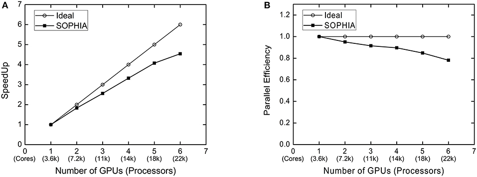
Figure 7. Performance scalability test of multi-GPU code. (A) Speedup factor of strong scaling and (B) efficiency of weak scaling.

Benchmark Analysis

As described in section Smoothed Particle Hydrodynamics (SPH), SOPHIA consists of various models such as hydrodynamics, heat transfer, turbulence, multi-phase flow, etc. Although all the details are not described in this paper, the code has conducted various basic V&V simulations including hydrostatic pressure, Poiseuille & Couette flow, lid-driven flow, 2D/3D dam break, 3D wave generation, hydrostatic pressure in immiscible fluids, the lock exchange problem, Rayleigh-Tayler instability, multi-dimensional heat conduction, and natural circulation. Some of the results are summarized in Jo et al. (2019) and Park et al. (2019). For the newly implemented physical models such as turbulence, chemical reaction, etc., the verification and validation processes are currently underway. In this section, the simulations are conducted on three benchmark experiments related to nuclear safety. The selected benchmark experiments are (1) water jet breakup of Fuel–Coolant Interaction (FCI), (2) Liquid Metal Reactor (LMR) centralized sloshing, and (3) bubble lift force.

Jet Breakup of Fuel–Coolant Interaction

Fuel–Coolant Interaction (FCI) is one of major phenomena of severe accidents and occurs when molten fuel falls into the coolant or vice versa. The interaction between coolant and the molten fuel involves many complicated physical phenomena, which may lead to a catastrophic event such as a steam explosion. Especially, jet breakup, where the bulk of molten fuel breaks into droplets, is the most important pre-mixing phase for a steam explosion or re-melting of fuel fragments, which threatens the reactor vessel/containment integrity (Allelein et al., 1999; Sehgal et al., 1999). In this study, an isothermal benchmark experiment on jet breakup conducted by Park et al. (2016) is simulated using the SOPHIA code and the results are discussed.

The impinging jet simulation model consists of a jet column and a tank filled with Fluorinert. The tank is a rectangular column of 0.1 m width, 0.02 m depth, and 0.4 m height, and the pool is filled up to a height of 0.2 m. As in the experiment, the rest of the tank is filled with the air in the simulation. The jet diameter is 10 mm. The water jet has a density of 1,000 kg/m³, a viscosity of 1.0 mPa · s, and a surface tension of 0.072 N/m and the Fluorinert pool has a density of 1,880 kg/m³, a viscosity of 4.7 mPa · s, and a surface tension of 0.043 N/m. The inlet jet velocity was set as 3.8 m/s. The total number of particles was 57,430,016. The simulation was conducted using six GPUs.

Figure 8 shows snapshots of the simulation. The jet, injected at a high velocity, penetrates into the pool. This penetration causes a U-shaped air pocket just behind the jet front. The interaction with the pool dissipates the initial momentum of the jet front, suspending further penetration. At the same time, the air pocket collapses due to the compression of the pool. The jet continuously drags the air into the pool and breaks up through the interaction with the pool. Mixing of jet droplets and air bubbles enhances the buoyant effect of the jet. As a result, the jet fails to penetrate below a certain depth, and the jet disperses out radially. According to previous studies (Ikeda et al., 2001; Park et al., 2016), it is noted that this jet breakup and fragmentation can only be modeled physically by three-dimensional two-phase flow simulation. This is because ignoring the air cavity may distort the consequent phenomena. As shown in Figure 8, such jet behavior is well-reproduced through the three-dimensional two-phase flow simulation with high resolution. Especially, in the simulation, the droplets are generated at the pool–jet–air interfaces by velocity differences (referred to as Kelvin-Helmholtz instability) or surface tension effects (referred to as critical Weber number theory).

FIGURE 8

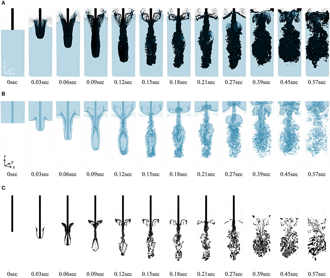
Figure 8. Snapshots of two-phase simulation of jet breakup: (A) two fluids with rendering (blue for the Fluorinert pool, and black for the water jet), (B) air with rendering, and (C) jet breakup behavior at the x–z plane.

For rigorous analysis, the simulation results are compared with experimental data in two ways: (1) jet penetration depth and (2) overall pool surface shape/level. Figure 9A compares the jet front penetration depth in the simulation with the experimental data. The jet front in the simulation shows very good agreement with the experimental data over time. Figure 9B compares the pool surface shape in the simulation and in the experiment (the red lines represent the surface of the experimental visual images at the same time). As shown in the figure, the simulation agrees very well with the experimental results, not only for the surface level but also in terms of the overall features.

FIGURE 9

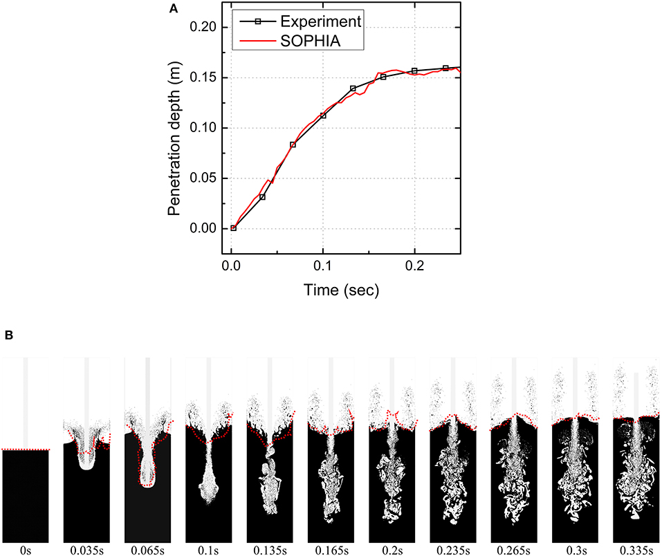
Figure 9. Comparison of the simulation results with the experimental results: (A) comparison of the jet penetration depth and (B) comparison of the pool surface level with the experimental visualization (red lines for experimental results; Park et al., 2016).

Liquid Metal Reactor Centralized Sloshing

In the transient phase of a core-disruptive Liquid Metal Reactor (LMR) accident, a neutronically active multi-phase pool can be formed, which is composed of solid fuel, molten fuel, re-frozen fuel, fission gas, fuel vapor, steel particles, etc. In this configuration, abrupt pressure build-up due to local vapor generation can initiate so-called centralized sloshing motion, which has the potential for energetic fuel re-criticalities (Suzuki et al., 2014). In this study, three-dimensional sloshing simulations are conducted using the SOPHIA code on the benchmark experiment by Maschek et al. (1992a).

The simulation model consists of a water column, a container, and 12 vertical rods. The container is an open cylinder with a 44-cm diameter. The water column, with 11 cm diameter and 20 cm height, is located in the center of the container. Regarding the vertical rods, which all have the same diameter of 2 cm, the three simulation cases were considered.

• Case 1 has no vertical rods but only the water column.

• Case 2 has inner vertical rods that surround the water column in a ring with a diameter of 19.8 cm.

• Case 3 has outer vertical rods that surround the water column in a ring with a diameter of 35.2 cm diameter.

Figure 10 shows the simulation results for Case 1, Case 2, and Case 3, respectively. In Case 1, the water column collapses due to gravity, and it makes a circular wave moving toward the container wall. After collision with the wall, the water converges toward the center area, and it forms a high central water peak. In Case 2 and Case 3, 12 vertical inner/outer rods are placed around the central water column. The simulations reproduce the damping and interference motion of water waves induced by rod disturbances well.

FIGURE 10

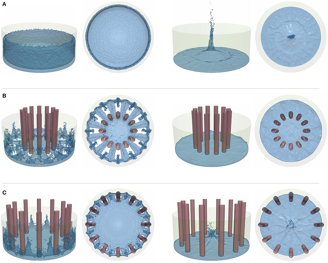
Figure 10. Snapshots of surface motion of the simulation cases with rendering: (A) Case 1 simulation results, (B) Case 2 simulation results, and (C) Case 3 simulation results.

In this study, the maximum sloshing height and arrival time in the simulations are compared with the experimental data, as shown in Table 4. The (1) arrival time, (2) time of maximum height, and (3) maximum height at the outer container wall and the pool center are taken into account. In general, the SOPHIA simulation results show very good agreement with the benchmark experimental data, both qualitatively and quantitatively.

TABLE 4

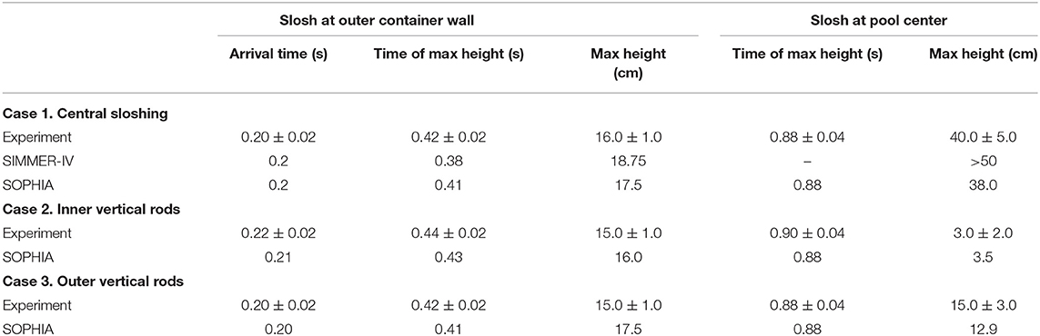
Table 4. Comparison of SOPHIA simulation with experiments (Maschek et al., 1992b; Pigny, 2010).

Bubble Lift Force

Bubbly flow plays an important role not only in Light Water Reactors (LWRs) but also in many industries because it involves large interfacial areas for heat and mass transfer. In recent multi-phase CFD analysis, the lift force is one of the important forces for tracing bubble dynamics because it greatly affects the spatial distribution of bubbles and void fractions. In nuclear safety analysis, the effect of lift force was noticed early on by observing an accumulation of gas near the wall in the pipe flow (Tomiyama et al., 2002; Ziegenhein et al., 2018). In conventional CFD analysis, the lift force is commonly considered by empirical correlations based on experimental data. In this study, the bubble lift force in laminar shear flow is simulated, referring to the benchmark experiment by Tomiyama et al. (2002), and the bubble trajectories are compared with the experimental data.

In the benchmark experiment, a tank was filled with a glycerol-water solution, and a belt was continuously rotated at a constant speed to induce simple shear flow. At the steady state, a single air bubble was released on the linear velocity gradient field through a nozzle tip. For the simulation, a stationary vertical wall is placed in the middle of the tank, and both sidewalls are set to have a constant velocity to generate simple shear flow as in the experiment. The tank is a rectangular cavity with 60-mm width and 0.5-m height, and it is divided into two channels with 30-mm width by the stationary wall. As in the experiment, the tank is filled with a glycerol-water solution, and the fluid flows rotating clockwise. After achieving steady-state shear flow, a single air bubble is injected at the left channel of the model. The glycerol-water solution has a density of 1,154 kg/m³ and a viscosity of 0.091 Pa · s. This study performed two-dimensional simulation with 518,259 particles. Regarding the velocity gradient (ω) and bubble diameter (d), four experimental cases were considered.

• Case 1 has a small velocity gradient (ω = 5.7 s⁻¹) and large bubble diameter (d = 5.54 mm).

• Case 2 has a large velocity gradient (ω = 6.2 s⁻¹) and large bubble diameter (d = 5.54 mm).

• Case 3 has a small velocity gradient (ω = 5.7 s⁻¹) and small bubble diameter (d =3.52 mm).

• Case 4 has a large velocity gradient (ω = 6.2 s⁻¹) and small bubble diameter (d = 3.52 mm).

Figure 11 presents the simulation results of four cases and validations. Figure 11A shows image sequences of the simulations. The left two figures are the results for a large bubble diameter (d = 5.54 mm) and the right two figures for a small bubble diameter (d = 3.52 mm). As shown in the figure, the large bubble drifts toward the left wall as it rises up, while the small bubble drifts toward the right wall. This is because the shear-induced lift force is most dominant for the small bubbles. At the surface of the bubble, a relative velocity gradient is generated by the linear shear flow, and this gradient drags the small bubble so that it rotates toward the large drag force (high velocity). However, for large bubbles, slanted-wake-induced lift force is more dominant than shear-induced lift force. When the large bubble floats through the linear shear flow, asymmetric wakes are formed right behind the bubble, and this wake configuration perturbs the surrounding pressure field. Due to the pressure gradient, the large bubble tends to move toward the lower velocity with deformation. Figure 11B compares the trajectories of the bubbles in the experiment and in the simulation. As shown in the figure, the simulation results are agreed very well with the experimental results within measurement error.

FIGURE 11

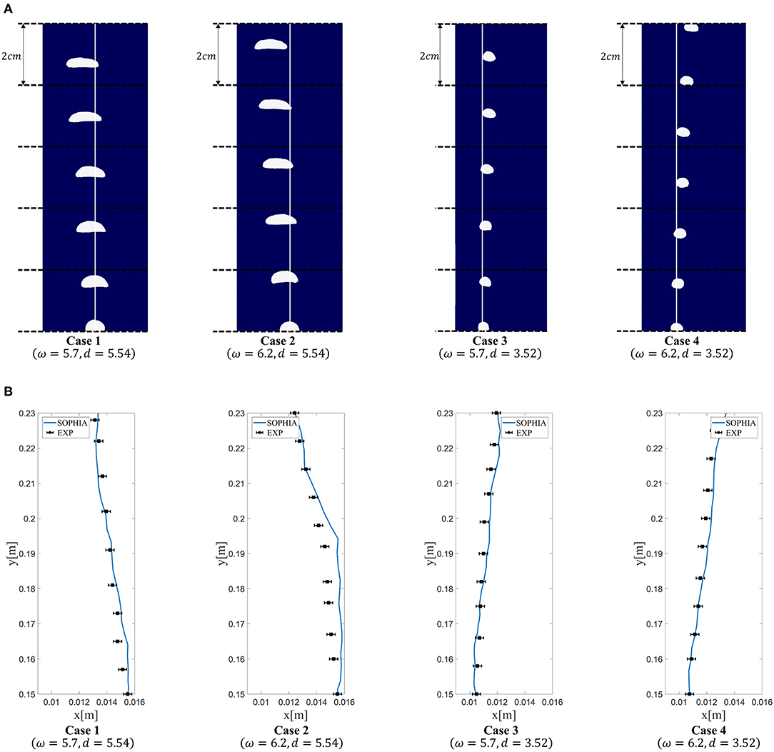
Figure 11. The simulation results for bubble lift force: (A) bubble floating sequence with rendering and (B) comparison of bubble trajectories with the experimental data (Tomiyama et al., 2002).

Summary and Conclusion

This paper summarizes the recent progress and on-going activity in the development of the Lagrangian-based CFD code (SOPHIA), with some demonstrations on nuclear applications. The SOPHIA code is based on the smoothed particle hydrodynamics (SPH), which is the most widely used full-Lagrangian method. Like other conventional CFD methods, the SOPHIA code basically solves mass, momentum, and energy conservation equations. However, unlike conventional SPH, the SOPHIA code formulates the density and the continuity equations in terms of normalized density in order to handle multi-phase, multi-fluid, and multi-component flows in a simple and effective manner. In addition, the SOPHIA code incorporates physical models, including fluid flow, heat transfer, mass transfer, multi-phase, phase change, turbulence, and diffusion, with various numerical correction schemes so that the code can be applied well to many different nuclear safety-related issues.

In spite of its great potential for nuclear thermal hydraulics and safety, the Lagrangian-based CFD still faces some technical challenges that need to be further addressed. One of the critical drawbacks of the SPH method is the high computational cost. In order to address this issue, this study implements the code using multi-GPU parallelization with various parallel computing techniques such as multi-threading, mapping, and sorting. The main algorithm consists of four steps: (1) multi-GPU allocation, (2) sub-domain division, (3) multi-GPU concurrent execution, and (4) inter-GPU communication. Especially, the multi-GPU concurrent execution step parallelizes the computation procedure into two streams to optimize calculation and memory exchange. The computational performance of the multi-GPU parallelized SOPHIA code is evaluated by both strong and weak scaling. The results indicate that SOPHIA code showed remarkable performance from small-scale to large-scale problems with an increase in the number of GPUs, and it reached 78% efficiency with a maximum six GPUs.

To demonstrate its applicability to nuclear thermal hydraulics and safety, three benchmark simulations were conducted: (1) water jet breakup of FCI, (2) LMR centralized core sloshing, and (3) bubble lift force. All of these simulations showed that the SOPHIA code can predict the key phenomena in the experiments, both qualitatively and quantitatively. According to the benchmark results and discussions, SPH methods such as the SOPHIA code seem to be well-suited to safety-related analysis (i.e., for severe accident and natural disaster), numerical experiments, and visualization of phenomena. All of these activities have a large potential to reduce the uncertainties regarding the phenomena related to decision-making.

Although the SOPHIA code has great potential in nuclear thermal hydraulics and safety analysis, technical challenges remain that require further investigations. The following lists some of the items that should be addressed in the future:

• Method for handling multi-scale problems (i.e., boiling, turbulence, etc.)

• Method for reducing large computational cost (i.e., optimization, numerical schemes)

• Method for handling various boundary conditions (i.e., symmetry, open boundary, etc.)

• Method for improving both accuracy and stability (i.e., numerical schemes)

• Method for verification and validation (i.e., benchmark experiment, visualization, etc.)

Data Availability Statement

All datasets generated for this study are included in the article/supplementary material.

Author Contributions

S-HP developed the code and performed simulations, analyzed data, and drafted or provided the revision of the paper. YJ and YA developed the code and performed simulations, analyzed data, and co-wrote the paper. HC, TC, S-SP, HY, and JK developed the code, performed simulations, and analyzed data. EK supervised the research and resolved appropriately, provided the revision of the paper, and approved of the final version to be published.

Funding

This research was supported by the Nuclear Energy Technology Development Program (U.S.-ROK I-NERI Program) through the National Research Foundation of Korea (NRF), funded by the Ministry of Science and ICT (2019M2A8A1000630), and the Nuclear Safety Research Program through the Korea Foundation of Nuclear Safety (KoFONS), using the financial resources granted by the Nuclear Safety and Security Commission (NSSC) of the Republic of Korea (No. 1903003).

Conflict of Interest

The authors declare that the research was conducted in the absence of any commercial or financial relationships that could be construed as a potential conflict of interest.

Abbreviations

AOS, Array of Structure; CFD, Computational Fluid Dynamics; CPU, Central Processing Unit; CSF, Continuum Surface Force; CSPM, Corrective Smoothed Particle Method; δ-SPH, Delta-Smoothed Particle Hydrodynamics; EOS, Equation of State; FCI, Fuel–Coolant Interaction; FDM, Finite Difference Method; FEM, Finite Element Method; FPM, Finite Particle Method; FVM, Finite Volume Method; GPGPU, General Purpose Graphics Processing Unit; GPU, Graphics Processing Unit; IPF, Inter-molecular Potential Force; IS, Interface Sharpness; ISPH, Incompressible Smoothed Particle Hydrodynamics; IVMR, In-Vessel Melt Retention; KGC, Kernel Gradient Correction; KGF, Kernel Gradient Free; LES, Large Eddy Simulation; LMR, Liquid Metal Reactor; LWR, Light Water Reactor; MCCI, Molten Corium Concrete Interaction; MIC, Many Integrated Core; NNPS, Nearest Neighbor Particle Search; P2P, Peer-to-Peer (GPU-to-GPU); RANS, Reynolds Average Navier-Stokes; RHS, Right-Hand Side; SPH, Smoothed Particle Hydrodynamics; SPS, Sub-Particle Scale; WCSPH, Weakly Compressible Smoothed Particle Hydrodynamics.

References

Allelein, H., Basu, S., Berthoud, G., Jacobs, H., Magallon, D., Petit, M., et al. (1999). Technical Opinion Paper on Fuel-Coolant Interaction (No. NEA-CSNI-R−1999-24). Organisation for Economic Co-Operation and Development-Nuclear Energy Agency.

Google Scholar

Antuono, M., Colagrossi, A., Marrone, S., and Molteni, D. (2010). Free-surface flows solved by means of SPH schemes with numerical diffusive terms. Comput. Phys. Commun. 181, 532–549. doi: 10.1016/j.cpc.2009.11.002

CrossRef Full Text | Google Scholar

Arnason, H., Petroff, C., and Yeh, H. (2009). Tsunami bore impingement onto a vertical column. J. Disaster Res. 4, 391–403. doi: 10.20965/jdr.2009.p0391

CrossRef Full Text

Barto, A. (2014). Consequence Study of a Beyond-Design-Basis Earthquake Affecting the Spent Fuel Pool for a U.S. Mark I Boiling Water Reactor. United States Nuclear Regulatory Commission, Office of Nuclear Regulatory Research.

Bauer, T. H., Wright, A. E., Robinson, W. R., Holland, J. W., and Rhodes, E. A. (1990). Behavior of modern metallic fuel in treat transient overpower tests. Nuclear Technol. 92, 325–352. doi: 10.13182/NT92-325

CrossRef Full Text | Google Scholar

Belytschko, T., Krongauz, Y., Organ, D., Fleming, M., and Krysl, P. (1996). Meshless methods: an overview and recent developments. Comput Methods Appl Mech. Eng. 139, 3–47. doi: 10.1016/S0045-7825(96)01078-X

CrossRef Full Text | Google Scholar

Bonet, J., and Lok, T. S. (1999). Variational and momentum preservation aspects of smooth particle hydrodynamic formulations. Comput. Methods Appl. Mech. Eng. 180, 97–115. doi: 10.1016/S0045-7825(99)00051-1

CrossRef Full Text | Google Scholar

Bonnet, J. M., Cranga, M., Vola, D., Marchetto, C., Kissane, M., Robledo, F., et al. (2017). State-of-the-Art Report on Molten Corium Concrete Interaction and Ex-Vessel Molten Core Coolability (No. NEA−7392). Organisation for Economic Co-Operation and Development.

Google Scholar

Brackbill, J. U., Kothe, D. B., and Zemach, C. (1992). A continuum method for modeling surface tension. J. Comput. Phys. 100, 335–354. doi: 10.1016/0021-9991(92)90240-Y

CrossRef Full Text | Google Scholar

Chen, J. K., and Beraun, J. E. (2000). A generalized smoothed particle hydrodynamics method for nonlinear dynamic problems. Comput. Methods Appl. Mech. Eng. 190, 225–239. doi: 10.1016/S0045-7825(99)00422-3

CrossRef Full Text | Google Scholar

Cleary, P. W. (1998). Modelling confined multi-material heat and mass flows using SPH. Appl. Math. Modell. 22, 981–993. doi: 10.1016/S0307-904X(98)10031-8

CrossRef Full Text | Google Scholar

Cummins, S. J., Silvester, T. B., and Cleary, P. W. (2012). Three-dimensional wave impact on a rigid structure using smoothed particle hydrodynamics. Int. J. Numer. Methods Fluids 68, 1471–1496. doi: 10.1002/fld.2539

CrossRef Full Text | Google Scholar

Dehnen, W., and Aly, H. (2012). Improving convergence in smoothed particle hydrodynamics simulations without pairing instability. Monthly Notices R. Astrono. Soc. 425, 1068–1082. doi: 10.1111/j.1365-2966.2012.21439.x

CrossRef Full Text | Google Scholar

Gingold, R. A., and Monaghan, J. J. (1977). Smoothed particle hydrodynamics: theory and application to non-spherical stars. Monthly Notices R. Astrono. Soc. 181, 375–389. doi: 10.1093/mnras/181.3.375

CrossRef Full Text | Google Scholar

Gomez-Gesteira, M., Rogers, B. D., Crespo, A. J., Dalrymple, R. A., Narayanaswamy, M., and Dominguez, J. M. (2012). SPHysics–development of a free-surface fluid solver–Part 1: theory and formulations. Comput. Geosci. 48, 289–299. doi: 10.1016/j.cageo.2012.02.029

CrossRef Full Text | Google Scholar

Grenier, N., Antuono, M., Colagrossi, A., Le Touzé, D., and Alessandrini, B. (2009). An Hamiltonian interface SPH formulation for multi-fluid and free surface flows. J. Comput. Phys. 228, 8380–8393. doi: 10.1016/j.jcp.2009.08.009

CrossRef Full Text | Google Scholar

Guo, X., Rogers, B. D., Lind, S., and Stansby, P. K. (2018). New massively parallel scheme for Incompressible Smoothed Particle Hydrodynamics (ISPH) for highly nonlinear and distorted flow. Comput. Phys. Commun. 233, 16–28. doi: 10.1016/j.cpc.2018.06.006

CrossRef Full Text | Google Scholar

Harada, T., and Howes, L. (2011). Introduction to GPU Radix Sort. Heterogeneous Computing with OpenCL (San Francisco, CA: Morgan Kaufmann).

Google Scholar

Hu, X. Y., and Adams, N. A. (2006). A multi-phase SPH method for macroscopic and mesoscopic flows. J. Comput. Phys. 213, 844–861. doi: 10.1016/j.jcp.2005.09.001

CrossRef Full Text | Google Scholar

Huang, C., Lei, J. M., Liu, M. B., and Peng, X. Y. (2016). An improved KGF-SPH with a novel discrete scheme of Laplacian operator for viscous incompressible fluid flows. Int. J. Numer. Methods Fluids 81, 377–396. doi: 10.1002/fld.4191

CrossRef Full Text | Google Scholar

Ikeda, H., Koshizuka, S., Oka, Y., Park, H. S., and Sugimoto, J. (2001). Numerical analysis of jet injection behavior for fuel-coolant interaction using particle method. J. Nuclear Sci. Technol. 38, 174–182. doi: 10.1080/18811248.2001.9715019

CrossRef Full Text | Google Scholar

Jo, Y. B., Park, S. H., Choi, H. Y., Jung, H. W., Kim, Y. J., and Kim, E. S. (2019). SOPHIA: Development of Lagrangian-based CFD code for nuclear thermal-hydraulics and safety applications. Ann. Nuclear Energy 124, 132–149. doi: 10.1016/j.anucene.2018.09.005

CrossRef Full Text | Google Scholar

Lind, S. J., Xu, R., Stansby, P. K., and Rogers, B. D. (2012). Incompressible smoothed particle hydrodynamics for free-surface flows: a generalised diffusion-based algorithm for stability and validations for impulsive flows and propagating waves. J. Comput. Phys. 231, 1499–1523. doi: 10.1016/j.jcp.2011.10.027

CrossRef Full Text | Google Scholar

Liu, G. R., and Liu, M. B. (2003). Smoothed Particle Hydrodynamics: A Meshfree Particle Method. World Scientific. doi: 10.1142/5340

CrossRef Full Text | Google Scholar

Liu, M. B., and Liu, G. R. (2006). Restoring particle consistency in smoothed particle hydrodynamics. Appl. Numer. Math. 56, 19–36. doi: 10.1016/j.apnum.2005.02.012

CrossRef Full Text | Google Scholar

Liu, M. B., Liu, G. R., and Lam, K. Y. (2003). Constructing smoothing functions in smoothed particle hydrodynamics with applications. J. Comput. Appl. Math. 155, 263–284. doi: 10.1016/S0377-0427(02)00869-5

CrossRef Full Text | Google Scholar

Lucy, L. B. (1977). A numerical approach to the testing of the fission hypothesis. Astrono. J. 82, 1013–1024. doi: 10.1086/112164

CrossRef Full Text | Google Scholar

Ma, W., Yuan, Y., and Sehgal, B. R. (2016). In-vessel melt retention of pressurized water reactors: historical review and future research needs. Engineering 2, 103–111. doi: 10.1016/J.ENG.2016.01.019

CrossRef Full Text | Google Scholar

Maschek, W., Munz, C. D., and Meyer, L. (1992a). Investigations of sloshing fluid motions in pools related to recriticalities in liquid-metal fast breeder reactor core meltdown accidents. Nuclear Technol. 98, 27–43. doi: 10.13182/NT92-A34648

CrossRef Full Text | Google Scholar

Maschek, W., Roth, A., Kirstahler, M., and Meyer, L. (1992b). Simulation experiments for centralized liquid sloshing motions. Kernforschungszentrum Karlsruhe, 5090 (Karlsruhe).

Google Scholar

Molteni, D., and Colagrossi, A. (2009). A simple procedure to improve the pressure evaluation in hydrodynamic context using the SPH. Comput. Phys. Commun. 180, 861–872. doi: 10.1016/j.cpc.2008.12.004

CrossRef Full Text | Google Scholar

Monaghan, J. J. (1992). Smoothed particle hydrodynamics. Ann. Rev. Astrono. Astrophys. 30, 543–574. doi: 10.1146/annurev.aa.30.090192.002551

CrossRef Full Text | Google Scholar

Monaghan, J. J. (1994). Simulating free surface flows with SPH. J. Comput. Phys. 110, 399–406. doi: 10.1006/jcph.1994.1034

CrossRef Full Text | Google Scholar

Monaghan, J. J. (2005). Smoothed particle hydrodynamics. Rep. Progr. Phys. 68:1703. doi: 10.1088/0034-4885/68/8/R01

CrossRef Full Text | Google Scholar

Morris, J. P. (2000). Simulating surface tension with smoothed particle hydrodynamics. Int. J. Numer. Methods Fluids 33, 333–353. doi: 10.1002/1097-0363(20000615)33:3<333::AID-FLD11>3.0.CO;2-7

CrossRef Full Text | Google Scholar

Morris, J. P., Fox, P. J., and Zhu, Y. (1997). Modeling low Reynolds number incompressible flows using SPH. J. Comput. Phys. 136, 214–226. doi: 10.1006/jcph.1997.5776

CrossRef Full Text | Google Scholar

Nishiura, D., Furuichi, M., and Sakaguchi, H. (2015). Computational performance of a smoothed particle hydrodynamics simulation for shared-memory parallel computing. Comput. Phys. Commun. 194, 18–32. doi: 10.1016/j.cpc.2015.04.006

CrossRef Full Text | Google Scholar

Park, S., Park, H. S., Jang, B. I., and Kim, H. J. (2016). 3-D simulation of plunging jet penetration into a denser liquid pool by the RD-MPS method. Nuclear Eng. Des. 299, 154–162. doi: 10.1016/j.nucengdes.2015.08.003

CrossRef Full Text | Google Scholar

Park, S.H., Chae, H., Jo, Y. B., and Kim, Y. S. (2019). “SPH for general density gradient driven flow,” in Proceedings of the 14th SPHERIC International Workshop (Exeter), 67–75.

Park, S. H., Choi, T. S., Choi, H. Y., Jo, Y. B., and Kim, E. S. (2018). Simulation of a laboratory-scale experiment for wave propagation and interaction with a structure of undersea topography near a nuclear power plant using a divergence-free SPH. Ann. Nuclear Energy 122, 340–351. doi: 10.1016/j.anucene.2018.08.045

CrossRef Full Text | Google Scholar

Pigny, S. L. (2010). Academic validation of multi-phase flow codes. Nucl. Eng. Design 240, 3819–3829. doi: 10.1016/j.nucengdes.2010.08.007

CrossRef Full Text | Google Scholar

Randles, P. W., and Libersky, L. D. (1996). Smoothed particle hydrodynamics: some recent improvements and applications. Comput. Methods Appl. Mech. Eng. 139, 375–408. doi: 10.1016/S0045-7825(96)01090-0

CrossRef Full Text | Google Scholar

Rogers, B. D., and Dalrymple, R. A. (2008). “SPH modeling of tsunami waves,” in Advanced Numerical Models for Simulating Tsunami Waves and Runup, Vol. 10, eds P. L.-F. Liu, H. Yeh, and C. Synolakis (World Scientific), 75–100. doi: 10.1142/9789812790910_0003

CrossRef Full Text | Google Scholar

Sehgal, B. R., Dinh, T. N., Nourgaliev, R. R., Bui, V. A., Green, J., Kolb, G., et al. (1999). Final Report for the'Melt-Vessel Interactions' Project. European Union R and TD Program 4th Framework. MVI project final research report (No. SKI-R−00-53). Swedish Nuclear Power Inspectorate.

Google Scholar

Shigorina, E., Kordilla, J., and Tartakovsky, A. M. (2017). Smoothed particle hydrodynamics study of the roughness effect on contact angle and droplet flow. Phys. Rev. E 96:033115. doi: 10.1103/PhysRevE.96.033115

PubMed Abstract | CrossRef Full Text | Google Scholar

Sun, P. N., Colagrossi, A., Marrone, S., Antuono, M., and Zhang, A. M. (2017). “Targeting viscous flows around solid body at high Reynolds numbers with the delta-plus-SPH model,” in Proceedings of 12th International SPHERIC Workshop (Ourense).

Suzuki, T., Kamiyama, K., Yamano, H., Kubo, S., Tobita, Y., Nakai, R., et al. (2014). A scenario of core disruptive accident for Japan sodium-cooled fast reactor to achieve in-vessel retention. J. Nucl. Sci. Technol. 51, 493–513. doi: 10.1080/00223131.2013.877405

CrossRef Full Text | Google Scholar

Tartakovsky, A., and Meakin, P. (2005). Modeling of surface tension and contact angles with smoothed particle hydrodynamics. Phys. Rev. E 72:026301. doi: 10.1103/PhysRevE.72.026301

PubMed Abstract | CrossRef Full Text | Google Scholar

Tomiyama, A., Tamai, H., Zun, I., and Hosokawa, S. (2002). Transverse migration of single bubbles in simple shear flows. Chem. Eng. Sci. 57, 1849–1858. doi: 10.1016/S0009-2509(02)00085-4

CrossRef Full Text | Google Scholar

Valdez-Balderas, D., Domínguez, J. M., Rogers, B. D., and Crespo, A. J. (2013). Towards accelerating smoothed particle hydrodynamics simulations for free-surface flows on multi-GPU clusters. J. Parallel Distr. Comput. 73, 1483–1493. doi: 10.1016/j.jpdc.2012.07.010

CrossRef Full Text | Google Scholar

Violeau, D., and Issa, R. (2007). Numerical modelling of complex turbulent free-surface flows with the SPH method: an overview. Int. J. Numer. Methods Fluids 53, 277–304. doi: 10.1002/fld.1292

CrossRef Full Text | Google Scholar

Wang, Z. B., Chen, R., Wang, H., Liao, Q., Zhu, X., and Li, S. Z. (2016). An overview of smoothed particle hydrodynamics for simulating multiphase flow. Appl. Math. Modell. 40, 9625–9655. doi: 10.1016/j.apm.2016.06.030

CrossRef Full Text | Google Scholar

Zhang, M. Y., Zhang, H., and Zheng, L. L. (2008). Simulation of droplet spreading, splashing and solidification using smoothed particle hydrodynamics method. Int. J. Heat Mass Transfer 51, 3410–3419. doi: 10.1016/j.ijheatmasstransfer.2007.11.009

CrossRef Full Text | Google Scholar

Zhang, N., Zheng, X., and Ma, Q. (2017). Updated smoothed particle hydrodynamics for simulating bending and compression failure progress of ice. Water 9:882. doi: 10.3390/w9110882

CrossRef Full Text | Google Scholar

Zhao, Y., Wilson, P. R., and Stevenson, J. D. (1996). Nonlinear 3-D dynamic time history analysis in the reracking modifications for a nuclear power plant. Nucl. Eng. Design 165, 199–211. doi: 10.1016/0029-5493(96)01197-1

CrossRef Full Text | Google Scholar

Ziegenhein, T., Tomiyama, A., and Lucas, D. (2018). A new measuring concept to determine the lift force for distorted bubbles in low Morton number system: results for air/water. Int. J. Multiphase Flow 108, 11–24. doi: 10.1016/j.ijmultiphaseflow.2018.06.012

CrossRef Full Text | Google Scholar

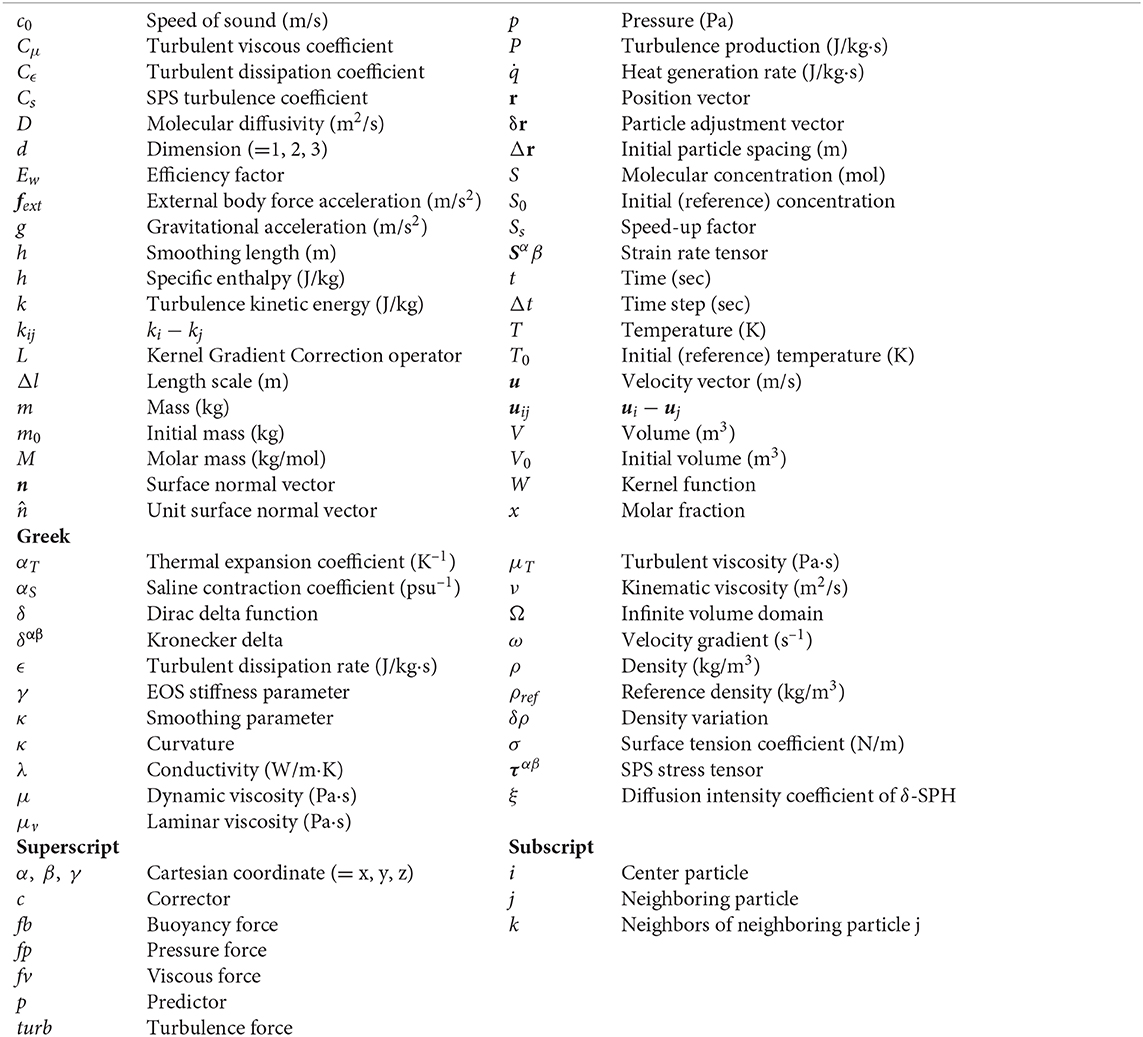
Nomenclature

Keywords: Lagrangian CFD, Smoothed Particle Hydrodynamics, multi-GPU parallelization, severe accident, Fuel Coolant Interaction, LMR core sloshing

Citation: Park S-H, Jo YB, Ahn Y, Choi HY, Choi TS, Park S-S, Yoo HS, Kim JW and Kim ES (2020) Development of Multi-GPU–Based Smoothed Particle Hydrodynamics Code for Nuclear Thermal Hydraulics and Safety: Potential and Challenges. Front. Energy Res. 8:86. doi: 10.3389/fenrg.2020.00086

Received: 12 January 2020; Accepted: 24 April 2020;
Published: 05 June 2020.

Edited by:

Victor Petrov, University of Michigan, United States

Reviewed by:

Xianping Zhong, University of Pittsburgh, United States
Jiankai Yu, Massachusetts Institute of Technology, United States
Rahim Shamsoddini, Sirjan University of Technology, Iran

Copyright © 2020 Park, Jo, Ahn, Choi, Choi, Park, Yoo, Kim and Kim. This is an open-access article distributed under the terms of the Creative Commons Attribution License (CC BY). The use, distribution or reproduction in other forums is permitted, provided the original author(s) and the copyright owner(s) are credited and that the original publication in this journal is cited, in accordance with accepted academic practice. No use, distribution or reproduction is permitted which does not comply with these terms.

*Correspondence: Eung Soo Kim, kes7741@snu.ac.kr

ORIGINAL RESEARCH article

Development of Multi-GPU–Based Smoothed Particle Hydrodynamics Code for Nuclear Thermal Hydraulics and Safety: Potential and Challenges

Introduction

Smoothed Particle Hydrodynamics (SPH)

Fundamentals of SPH

Governing Equations of the SOPHIA Code

Continuity Equation (Mass Conservation)

Navier-Stokes Equation (Momentum Conservation)

1st Law of Thermodynamics (Energy Conservation)

Equation of State

Turbulence

Molecular Diffusion

Buoyancy Force

Surface Tension

Multi-Phase Flow

Particle Shifting

Time Integration

Code Implementation

GPU Implementation

Basic Algorithm

Multi-GPU Allocation

Sub-domain Division

Concurrent Execution

Inter-GPU Communication

Evaluation of Multi-GPU Parallel Performance

Benchmark Analysis

Jet Breakup of Fuel–Coolant Interaction

Liquid Metal Reactor Centralized Sloshing

Bubble Lift Force

Summary and Conclusion

Data Availability Statement

Author Contributions

Funding

Conflict of Interest

Abbreviations

References

Nomenclature

This article is part of the Research Topic

People also looked at