Transport Ratios of the Kinetic Alfvén Mode in Space Plasmas

Narita, Yasuhito; Roberts, Owen Wyn; Vörös, Zoltán; Hoshino, Masahiro

doi:10.3389/fphy.2020.00166

PERSPECTIVE article

Front. Phys., 29 May 2020
Sec. Space Physics
Volume 8 - 2020 | https://doi.org/10.3389/fphy.2020.00166

Transport Ratios of the Kinetic Alfvén Mode in Space Plasmas

Yasuhito Narita¹^*

Owen Wyn Roberts¹

Zoltán Vörös^1,2

Masahiro Hoshino³

¹Space Research Institute, Austrian Academy of Sciences, Graz, Austria
²Research Centre for Astronomy and Earth Sciences, Geodetic and Geophysical Institute, Sopron, Hungary
³Graduate School of Science, The University of Tokyo, Tokyo, Japan

Fluctuation properties of the kinetic Alfvén mode, such as polarization of the wave electric and magnetic field around the mean magnetic field, parallel fluctuation to the mean field, ratios of the electric to magnetic field, and density fluctuations are analytically estimated by constructing the dielectric tensor of plasma based on the linear Vlasov theory. The dielectric tensor contains various fluid-picture processes in the lowest order, including polarization drift, Hall current, and diamagnetic current. Major discoveries from the dielectric tensor method in the kinetic Alfvén mode study are (1) identification of the mechanism of the field rotation sense reversal as a result of competition between the Hall and diamagnetic currents, (2) behavior of the parallel magnetic field fluctuation (in the compressive sense). The analytic expression of transport ratios serves as a diagnostic tool to study and identify the kinetic Alfvén mode in space plasma observations in the inner heliospheric domain.

1. Introduction

Kinetic Alfvén mode is one of the small-scale variants of the shear Alfvén mode in which the electric field parallel to the mean magnetic field direction (excited nearly in the electromagnetic fashion) is balanced against the electron-scale Debye screening when the wavevector becomes nearly perpendicular to the mean field [1]. The kinetic Alfvén mode is considered to play an important role in various space plasma environments and is one of the likely fluctuation constituents in solar wind turbulence. Indeed, various in situ observations of the solar wind plasma and magnetic field are favorably interpreted as a realization of the kinetic Alfvén mode from 0.1 to 100 Hz in the spacecraft frame (e.g., [2–8]).

The properties of the kinetic Alfvén mode and its possible realization in solar wind turbulence has also been investigated in numerical experiments [9–21]. In particular, explicit use of spectral ratios in order to characterize kinetic-scale fluctuations has been extensively used in recent kinetic simulations [22–28]. Discussion in Grošelj et al. [28] on the wave-like or coherent-structure nature of the sub-ion-scale fluctuations is of great interest in understanding the solar wind microphysics.

Here we revisit the kinetic Alfvén mode and analytically derive the transport ratios and scaling laws for the electric and magnetic fields in the spirit of developing useful tools for the wave mode identification in the spacecraft observations, particularly in view of the inner heliospheric observations, such as Parker Solar Probe, Solar Orbiter, and BepiColombo's cruise to Mercury. Our derivation is based on the dielectric tensor in the kinetic picture, and treat the dielectric tensor analytically in the leading orders so that the fluid picture properties of kinetic Alfvén mode are derived from the kinetic treatment. We fill the gap between the kinetic derivation and the fluid picture of kinetic Alfvén waves presented in Hollweg [29] by identifying various terms in the dielectric tensor that are physically relevant to the fluid picture, such as the polarization drift, Hall effect, and diamagnetic current.

2. Dielectric Response Framework

2.1. Dielectric Tensor

Our starting point is the dielectric tensor ϵ in the linear Vlasov theory, which gives the dispersion relation through the determinant-zero equation for the wave electric field, $D (\vec{k}, ω) \cdot \vec{E} = 0$ , or explicitly (cf. Equation 73, Chapter 10 in Stix [30]),

\begin{array}{l} [\begin{matrix} ϵ_{xx} - N_{‖}^{2} & ϵ_{xy} & ϵ_{xz} + N_{‖} N_{⊥} \\ - ϵ_{xy} & ϵ_{yy} - N^{2} & ϵ_{yz} \\ ϵ_{xz} + N_{‖} N_{⊥} & - ϵ_{yz} & ϵ_{zz} - N_{⊥}^{2} \end{matrix}] [\begin{matrix} E_{x} \\ E_{y} \\ E_{z} \end{matrix}] = 0 . & (1) \end{array}

Here the dispersion matrix D depends on the refraction indices N_‖ = k_‖c/ω, N_⊥ = k_⊥c/ω, and N = kc/ω, and most importantly, the dielectric tensor ϵ. A total refraction index, $N^{2} = N_{⊥}^{2} + N_{‖}^{2}$ , appears in the diagonal elements in Equation (1). We use the coordinate system spanning the mean magnetic field in the z-direction and the wavevector in the x-z-plane (denoted by $\vec{k} = (k_{x}, 0, k_{z}) = k_{⊥}, 0, k_{‖})$ ). Frequencies are assumed to be sufficiently smaller than the ion cyclotron frequency, ω ≪ Ω_i, where Ω_i = eB₀/m_i. Wavevectors are highly oblique to the mean magnetic field such that k_‖ ≪ k_⊥ holds.

Essential information on the wave properties is included in the dielectric tensor, e.g., dispersion relation, fluctuation sense of the wave electric and magnetic field. The elements of dielectric tensor for the kinetic Alfvén mode are evaluated in the paper by Lysak and Lotko [31], which can be simplified in the following way in the spirit of deriving the fluid-picture property of the wave

\begin{array}{l} ϵ_{xx} = 1 + \frac{c^{2}}{V_{A}^{2}} (1 - \frac{3}{4} μ_{i}) & (2) \end{array}

\begin{array}{l} ϵ_{yy} = 1 + \frac{c^{2}}{V_{A}^{2}} - \frac{β}{2} \frac{k_{⊥}^{2} c^{2}}{ω^{2}} & (3) \end{array}

\begin{array}{l} ϵ_{zz} = 1 + \frac{1}{k_{‖}^{2} λ_{De}^{2}} & (4) \end{array}

\begin{array}{l} ϵ_{xy} = i \frac{c^{2}}{V_{A}^{2}} \frac{Ω_{i}}{ω} (- 1 + \frac{3}{2} μ_{i}) & (5) \end{array}

\begin{array}{l} ϵ_{yz} = - \frac{i}{2} \frac{k_{⊥}}{k_{‖}} \frac{c^{2}}{V_{A}^{2}} \frac{Ω_{i}}{ω} (- 1 + \frac{3}{2} μ_{i}) = - \frac{1}{2} \frac{k_{⊥}}{k_{‖}} ϵ_{xy} & (6) \end{array}

\begin{array}{l} ϵ_{xz} = - \frac{1}{2} \frac{c^{2}}{V_{A}^{2}} \frac{k_{‖}}{k_{⊥}} μ_{i} . & (7) \end{array}

Here, ϵ_xx represents an extended form of the current for the polarization drift $c^{2} / V_{A}^{2}$ by correcting for the thermal motion in the perpendicular direction. The argument μ_i is defined as $μ_{i} = k_{⊥}^{2} r_{gi}^{2}$ , which is the square of the perpendicular wavenumbers normalized to the gyroradius of the thermal ions r_gi = v_{th, i}/Ω_i (here $v_{th, i} = {(k_{B} T_{i} / m_{i})}^{1 / 2}$ is the ion thermal speed and Ω_i the ion gyro-frequency). The plasma beta β is defined for both ions and electrons in an additive way, $β = 2 μ_{0} n k_{B} (T_{i} + T_{e}) / B_{0}^{2}$ . Quasi-neutrality is assumed, too.

The dielectric tensor method has been used in order to derive the properties of kinetic Alfvén mode fluctuations [32–36]. For example, Boldyrev et al. [34] presents the dielectric tensor method for both the kinetic Alfvén and the whistler modes. Passot and Sulem [36] discuss limits and full expressions for certain fluctuations. Our approach puts an emphasis on retaining the thermal correction (finite Larmor radius) to the polarization current in ϵ_xx (Equation 2) and extending the kinetic Alfvén mode to higher frequencies at about the ion cyclotron frequency in ϵ_yy, ϵ_xy, and ϵ_yz (Equations 3–6). We also use the notation with the Alfvén speed in the dielectric tensor using the relation $c^{2} / V_{A}^{2} = ω_{pi}^{2} / Ω_{i}^{2}$ , where ω_pi and Ω_i denote the ion plasma frequency and ion cyclotron frequency, respectively.

We treat a low-beta plasma case in deriving the properties of kinetic Alfvén mode. The diagonal elements of the dielectric tensor represent the plasma response for three different modes in the low-frequency domain: ϵ_xx represents the shear Alfvén mode (through the polarization drift), ϵ_yy the fast magnetosonic mode, and ϵ_zz the ion acoustic mode, respectively. The off-diagonal elements represent couplings among these modes. In particular, the first term in ϵ_xy represents a coupling of the Alfvén mode (incompressible mode) with the fast mode (compressible mode) through the Hall current and the second term a coupling through the diamagnetic current (see Appendix A for the comparison with the fluid picture). The off-diagonal elements relative to the diagonal elements become increasingly more important at shorter wavelengths. For example, the ratio of the xy to xx elements increases quadratically as a function of the perpendicular wavenumber in the dispersive range (retaining the diamagnetic current and simplifying the dispersion relation into $ω^{2} = k_{‖}^{2} V_{A}^{2} k_{⊥}^{2} r_{gi}^{2} (\frac{3}{4} + \frac{T_{e}}{T_{i}})$ ) as

\begin{array}{l} | \frac{ϵ_{xy}^{(dm)}}{ϵ_{xx}} | ≃ \frac{3}{2} tan θ \frac{v_{th, i}}{V_{A}} {(\frac{3}{4} + \frac{T_{e}}{T_{i}})}^{- 1 / 2} (1 + \frac{3}{4} k_{⊥}^{2} r_{gi}^{2}), & (8) \end{array}

while the ratio in the MHD range (retaining the Hall term and simplifying the dispersion relation into $ω^{2} = k_{‖}^{2} V_{A}$ ) is estimated as

\begin{array}{l} | \frac{ϵ_{xy}^{(h)}}{ϵ_{xx}} | ≃ \frac{Ω_{i}}{ω} ≃ \frac{Ω_{i}}{k_{‖} V_{A}} . & (9) \end{array}

The dispersion relation is obtained by decoupling of the fast mode from the Alfvén mode and solving the determinant-zero equation for the xx, xz, zx, and zz elements [31].

The dispersion relation of kinetic Alfvén mode is obtained by decoupling from the fast mode (represented by the yy element) and solving the reduced equation containing the Alfvén mode fluctuation or polarization drift (represented by the xx element) and the parallel electron motion (represented by the zz element):

\begin{array}{l} [\begin{matrix} ϵ_{xx} - N_{‖}^{2} & ϵ_{xz} + N_{‖} N_{⊥} \\ ϵ_{xz} + N_{‖} N_{⊥} & ϵ_{zz} - N_{⊥}^{2} \end{matrix}] [\begin{matrix} E_{x} \\ E_{z} \end{matrix}] . & (10) \end{array}

Furthermore, if the coupling term ϵ_xz is neglected since the wavevector is nearly perpendicular to the mean magnetic field, the determinant-zero condition is obtained as

\begin{array}{l} ϵ_{xx} ϵ_{zz} - N_{‖}^{2} ϵ_{zz} - N_{⊥}^{2} ϵ_{xx} = 0, & (11) \end{array}

from which the dispersion relation reads (Equation 2.44 in Hasegawa and Uberoi [1]):

\begin{array}{l} ω^{2} = k_{‖}^{2} V_{A}^{2} [1 + k_{⊥}^{2} r_{gi}^{2} (\frac{3}{4} + \frac{T_{e}}{T_{i}})] . & (12) \end{array}

The electron temperature is higher than the proton temperature in the low-speed solar wind (up to a ratio of 4) and lower in the high-speed solar wind (down to about 0.7) [37], with a mean value of T_e/T_i = 1.64 and a median of T_e/T_i = 1.27 [38].

If the thermal correction is neglected in the polarization current (i.e., in low-beta plasmas), the dispersion relation is simplified into the following form (Equation E18 in Schekochihin et al. [32]; see also Bian et al. [33], or Passot and Sulem [36]):

\begin{array}{l} ω^{2} = k_{‖}^{2} V_{A}^{2} (1 + k_{⊥}^{2} ρ_{s}^{2}), & (13) \end{array}

where ρ_s is ion-sound gyro-radius or sonic Larmor radius defined as

\begin{array}{l} ρ_{s}^{2} = \frac{T_{e}}{T_{i}} r_{gi}^{2} . & (14) \end{array}

The concept of ion-sound radius was introduced in the studies of magnetic reconnection during the late 1960's to early 1970's.

At higher values of beta, thermal correction is needed by keeping the coupling ϵ_xz, and in that case, the dispersion relation is extended to the following form

\begin{array}{l} ω^{2} = k_{‖}^{2} V_{A}^{2} [1 + k_{⊥}^{2} r_{gi}^{2} [\frac{3}{4} + \frac{T_{e}}{T_{i}} - k_{‖}^{2} r_{gi}^{2} \frac{T_{e}}{T_{i}} (1 + \frac{3}{4} k_{⊥}^{2} r_{gi}^{2})]] . & (15) \end{array}

The dispersion relation of kinetic Alfvén mode (Equation 15) is graphically presented in Figure 1 for different values of ion beta and propagation angles to the mean magnetic field. The conventional expression (Equation 12) is valid up to wavenumbers of k_⊥r_gi ~ 3.

FIGURE 1

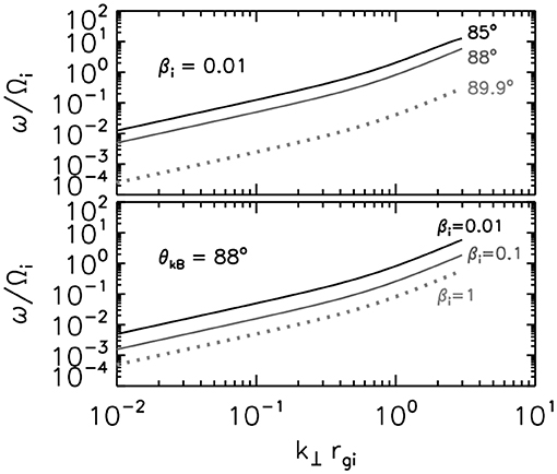
Figure 1. Dispersion relation of kinetic Alfvén mode for different values of ion beta (top) and propagation angles to the mean magnetic field (bottom). Electron-to-ion temperature ratio is set to unity.

Condition of a constant propagation angle (which is observationally supported by multi-spacecraft wave analyses of solar wind fluctuations, such as Perschke et al. [39] and Roberts et al. [40]) is applied in Figure 1. The parallel and perpendicular components of the wavevector are related to the wavevector magnitude by k_‖ = k cos θ and k_⊥ = k sin θ, respectively. Different options are possible to plot the dispersion relations. For example, the frequency can be divided by the product of parallel wavenumber and Alfvén speed as ω/(k_‖V_A) [32]; the dispersion relation may be simplified into ω∝k_‖k_⊥ irrespective of wavevector anisotropy [41]; application of critical balance [42]; and intermittency correction [20].

2.2. Transport Ratios

2.2.1. Electric Field Polarization

Electric field polarization (field rotation sense around the mean magnetic field) is evaluated by the ratio of the two perpendicular field components, and can directly be obtained from the dispersion tensor as follows:

\begin{array}{l} \frac{E_{y}}{E_{x}} = \frac{D_{xz} D_{yx} - D_{xx} D_{yz}}{D_{xy} D_{yz} - D_{xz} D_{yy}} & (16) \end{array}

\begin{array}{l} = \frac{- (ϵ_{xz} + N_{‖} N_{⊥}) ϵ_{xy} - (ϵ_{xx} - N_{‖}^{2}) ϵ_{yz}}{ϵ_{xy} ϵ_{yz} - (ϵ_{xz} + N_{‖} N_{⊥}) (ϵ_{yy} - N^{2})}, & (17) \end{array}

where the dielectric tensor in Equations (2)–(7) is used in deriving Equation (17). Since the yz element of dielectric tensor is proportional to the xy element (Equation 6), the polarization E_y/E_x is proportional to the xy element, E_y/E_x ∝ ϵ_xy. Change in sense of field rotation is hence associated with the competition between the Hall current and the diamagnetic current.

A more complete expression of the electric field polarization is shown in Appendix B. Approximation at lower wavenumbers k_⊥r_gi < 1 yet kd_i > 1, where d_i = V_A/Ω_i is the ion inertial length) yields a left-hand polarization (though polarization is highly elliptic)

\begin{array}{l} \frac{E_{y}}{E_{x}} ≃ i \frac{k_{‖} d_{i}}{k^{2} d_{i}^{2}} & (18) \end{array}

\begin{array}{l} ≃ i \frac{cos θ}{k d_{i}} . & (19) \end{array}

and approximation at higher wavenumbers (k_⊥r_gi > 1) yields a right-hand sense of polarization:

\begin{array}{l} \frac{E_{y}}{E_{x}} ≃ i \frac{3}{4} \frac{v_{th, i}^{2}}{V_{A}^{2}} \frac{ω^{3}}{Ω_{i}^{3}} (1 - \frac{3}{4} k_{⊥}^{2} r_{gi}^{2}) & (20) \end{array}

\begin{array}{l} ~ - i \frac{9}{16} \frac{v_{th, i}^{4}}{V_{A}^{4}} \frac{ω^{3}}{Ω_{i}^{3}} {tan}^{2} θ . & (21) \end{array}

Electric field polarization is plotted in the top panel of Figure 2 for the full expression (Equation 17) and the two approximations (Equations 17 and 21).

FIGURE 2

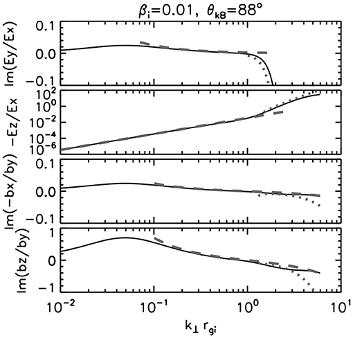
Figure 2. Electric field polarization, parallel electric field, magnetic field polarization, and parallel magnetic field as a function of the perpendicular component of wavevector normalized to the thermal ion gyro-radius. Ion beta 0.01. Propagation angle 88° to the mean magnetic field. Dashed and dotted curves are the low-wavenumber and high-wavenumber approximations, respectively. Electron-to-ion temperature ratio is set to unity. Equations (18), (30), (36), (45) are used for the low-wavenumber approximation (dashed lines). Equations (21), (31), (39), (46) are used for the high-wavenumber approximation (dotted lines).

Dependence on the propagation angle $θ_{kB} = {tan}^{- 1} (k_{⊥} / k_{‖})$ and the plasma beta (for ions) is displayed in the top panels of Figures 3, 4, respectively. Electric field has a left-hand rotation sense around the mean magnetic field at lower wavenumbers and changes into right-hand rotation sense at $k_{⊥} r_{gi} = \sqrt{2 / 3} ≃ 0.816$ and above (marked by vertical dotted lines in Figures 3, 4).

FIGURE 3

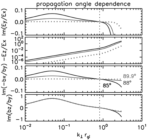
Figure 3. Transport ratios for different values of propagation angle to the mean magnetic field. The parameter set is taken from Figure 2.

FIGURE 4

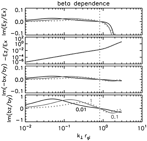
Figure 4. Transport ratios for different values of ion beta. The parameter set is taken from Figure 2.

The fluid-picture of field polarization is associated with a simplified version of Equation (17):

\begin{array}{l} \frac{E_{y}}{E_{x}} = - \frac{ϵ_{xy}}{N^{2}} & (22) \end{array}

\begin{array}{l} ~ - i \frac{ω}{Ω_{i}} \frac{Ω_{i}^{2}}{k^{2} V_{A}^{2}} (- 1 + \frac{3}{2} k_{⊥}^{2} r_{gi}^{2}) & (23) \end{array}

Again, Equation (22) shows that the rotation sense of the wave electric field depends on the sign of the dielectric response ϵ_xy, which is a combination of the Hall current with the diamagnetic current.

If the diamagnetic current dominates the dielectric response (or equivalently, when the perpendicular wavenumber is sufficiently large and the electron temperature is lower than that of ions the electric field polarization reduces to that in the fluid picture,

\begin{array}{l} \frac{E_{y}}{E_{x}} = - \frac{ϵ_{xy}^{(dm)}}{N^{2}} & (24) \end{array}

\begin{array}{l} = - i \frac{3}{2} \frac{ω}{Ω_{i}} \frac{Ω_{i}^{2}}{k^{2} V_{A}^{2}} k_{⊥}^{2} r_{gi}^{2} & (25) \end{array}

\begin{array}{l} = - i \frac{3}{2} \frac{ω}{Ω_{i}} \frac{v_{th, i}^{2}}{V_{A}^{2}} & (26) \end{array}

Equation (23) can be compared with that obtained from the fluid-theoretical approach Equation (46) in Hollweg [29]. Note that Equation (23) is a measure of the out-of-plane component of electric field (to the plane spanning the mean magnetic field and the wavevector) relative to the in-plane component. The inversion of E_y/E_x from Hollweg's result reflects different choices of the coordinate system Hollweg's paper takes the perpendicular component of wavevector as the y direction, while our paper takes that component as the x direction. The factor 3/2 in Equation 23) originates in the different use of temperature. Hollweg's paper uses the temperature through the sound speed c_s by including both the ion and the electrons thermal motions with the respective polytropic index γ, while our paper uses the temperature through the ion thermal speed. Our paper does not include the electron thermal effect (such as diamagnetic drift) in the perpendicular direction. Hollweg's result is obtained by replacing $3 / 2 v_{th, i}^{2}$ by $c_{s}^{2}$ . The factor 3/2 them arises when considering the longitudinal ion motion in the ion sound speed (which makes a factor of γ = 3) and the two perpendicular components (x and y components) in the ion gyro-motion in the definition of ion thermal speed (which makes a factor of 1/2). Field (temporal) rotation is right-hand, which has the same sense as electron gyro-motion as presented by Gary [43] and Hollweg [29]. If the Hall current dominates, however, the field rotation flips to the left-hand polarized sense.

2.2.2. Parallel Electric Field

The parallel component of electric field is obtained in the same fashion as the polarization in the xy plane. The relation to the dielectric (or dispersion) tensor is

\begin{array}{l} \frac{E_{z}}{E_{x}} = \frac{D_{xy} D_{zx} - D_{xx} D_{zy}}{D_{xz} D_{zy} - D_{xy} D_{zz}} . & (27) \end{array}

Again, the full expression of the ratio E_z/E_x is shown in Appendix B. If the value of beta is sufficiently low, the parallel ratio E_z/E_x is expressed as:

\begin{array}{l} \frac{E_{z}}{E_{x}} = - \frac{k_{‖}}{k_{⊥}} [\frac{3}{2} - \frac{1}{2} \frac{ω^{2}}{k_{‖}^{2} V_{A}^{2}} (1 - \frac{3}{4} k_{⊥}^{2} r_{gi}^{2})] \times \\ {[- \frac{3}{2} + \frac{ω^{2}}{k_{‖}^{2} V_{A}^{2}} \frac{1}{k_{⊥}^{2} r_{gi}^{2} T_{e} / T_{i}}]}^{- 1} . & (28) \end{array}

Approximation at lower wavenumbers (k_⊥r_gi < 1) is

\begin{array}{l} \frac{E_{z}}{E_{x}} ≃ - \frac{T_{e}}{T_{i}} k_{‖} k_{⊥} r_{gi}^{2} & (29) \end{array}

\begin{array}{l} ≃ - tan θ \frac{T_{e}}{T_{i}} k_{⊥}^{2} r_{gi}^{2} & (30) \end{array}

and that at higher wavenumbers (k_⊥r_gi > 1) is

\begin{array}{l} \frac{E_{z}}{E_{x}} ≃ \frac{1}{2 tan θ} (\frac{3}{4} + \frac{T_{e}}{T_{i}}) {[- \frac{3}{2} + (\frac{3}{4} + \frac{T_{e}}{T_{i}}) {(\frac{T_{e}}{T_{i}})}^{- 1}]}^{- 1} \times \\ k_{⊥}^{2} r_{gi}^{2} (1 - \frac{3}{4} k_{⊥}^{2} r_{gi}^{2}) . & (31) \end{array}

Equations (28), (30), and (31) are displayed in the second panel of Figure 2. The parallel electric field becomes more significant at larger wavenumbers, and exceeds the perpendicular electric field when k_⊥r_gi > 2, particularly when the wavevector has a moderate deviation from the perpendicular direction (e.g., 85 and 88° in Figure 3 irrespective of the values of beta (Figure 4).

The fluid-approach derivation by Hollweg [29] is obtained as follows:

\begin{array}{l} \frac{E_{z}}{E_{x}} = - \frac{N_{‖} N_{⊥} - N_{‖}^{2} (\frac{ω^{2}}{k_{‖} V_{A}^{2}} - 1) \frac{1}{2} \frac{k_{⊥}}{k_{‖}}}{(\frac{1}{k_{‖}^{2} λ_{De}^{2}} - N_{⊥}^{2} - N_{‖} N_{⊥} \frac{1}{2} \frac{k_{⊥}}{k_{‖}})} & (32) \end{array}

\begin{array}{l} = \frac{(\frac{m_{e}}{m_{i}} \frac{ω^{2}}{k_{‖}^{2}} \frac{v_{th, e}^{2}}{V_{A}^{2}} - \frac{k_{B} T_{e}}{m_{i}}) k_{‖} k_{⊥}}{Ω_{i}^{2} (1 + k_{⊥}^{2} ρ_{L}^{2})} & (33) \end{array}

The low-wavenumber approximation can be derived in a more simplified way:

\begin{array}{l} \frac{E_{z}}{E_{x}} ≃ - \frac{D_{zx}}{D_{zz}} = - \frac{T_{e}}{T_{i}} k_{‖} k_{⊥} r_{gi}^{2} . & (34) \end{array}

Equation (34) reproduces the second term (leading term) in Equation (16) in Hollweg [29]. The parallel electric field expression E_z/E_x enters directly the dispersion relation, and is essentially proportional to k_‖k_⊥ normalized to the (fictitious) ion gyroradius using the electron temperature.

2.2.3. Magnetic Field Polarization

Magnetic field polarization is related to the parallel electric field E_z/E_x and the electric field polarization E_y/E_x through the induction equation, $δ \vec{B} = ω^{- 1} \vec{k} \times \vec{E}$ . By noting that the wavevector is in the x–z plane, $\vec{k} = (k_{⊥}, 0, k_{‖})$ , we define the magnetic field polarization as the imaginary part of −δB_x/δB_y because δB_y is the most significant component in the fluctuating magnetic field. In the definition above, the positive value of imaginary part of −δB_x/δB_y corresponds to the left-hand (temporal) rotation sense around the mean magnetic field in an agreement with the construction of the electric field polarization. We obtain the magnetic field polarization as follows.

\begin{array}{l} - \frac{δ B_{x}}{δ B_{y}} = \frac{E_{y}}{E_{x}} {(1 - \frac{k_{⊥}}{k_{‖}} \frac{E_{z}}{E_{x}})}^{- 1} . & (35) \end{array}

At lower wavenumbers (k_⊥r_gi < 1), the polarization is obtained using Equations (18) and (29) as:

\begin{array}{l} - \frac{δ B_{x}}{δ B_{y}} ≃ i \frac{1}{tan θ} \frac{1}{k d_{i}} (1 - \frac{T_{e}}{T_{i}} k_{⊥}^{2} r_{gi}^{2}) . & (36) \end{array}

In fact, Equation (36) turns out to be a valid expression even at higher wavenumbers (k_⊥r_gi > 1) (dashed line in the third panel of Figure 2). In the fluid picture, when the diamagnetic current dominates at higher wavenumbers, the magnetic field polarization is obtained in a simpler way from Equations (26) and (34):

\begin{array}{l} - \frac{δ B_{x}}{δ B_{y}} = - i \frac{3}{2} \frac{v_{th, i}^{2}}{V_{A}^{2}} \frac{ω}{Ω_{i}} {(1 + \frac{T_{e}}{T_{i}} k_{⊥}^{2} r_{gi}^{2})}^{- 1} & (37) \end{array}

\begin{array}{l} ≃ - i \frac{3}{2} \frac{k_{‖}^{2} v_{th, i}^{2}}{ω Ω_{i}}, & (38) \end{array}

where the frequency is approximated to $ω ~ k_{‖} V_{A} (1 + k_{⊥} r_{gi} {(T_{e} / T_{i})}^{1 / 2})$ in Equation (38). The polarization at higher wavenumbers (k_⊥r_gi > 1) is obtained using Equations (21) and (31) as:

\begin{array}{l} - \frac{δ B_{x}}{δ B_{y}} ≃ i \frac{9}{16} \frac{v_{th, i}^{4}}{V_{A}^{4}} \frac{ω^{3}}{Ω_{i}^{3}} \frac{{tan}^{2} θ}{C k_{⊥}^{2} r_{gi}^{2} (1 - \frac{3}{4} k_{⊥}^{2} r_{gi}^{2})}, & (39) \end{array}

where the coefficient C is a numerical factor defined as

\begin{array}{l} C = \frac{1}{2} (\frac{3}{4} + \frac{T_{e}}{T_{i}}) {[- \frac{3}{2} + (\frac{3}{4} + \frac{T_{e}}{T_{i}}) {(\frac{T_{e}}{T_{i}})}^{- 1}]}^{- 1} . & (40) \end{array}

Equation (39), however, turns out to be valid only in a narrow range of wavenumbers (dotted line for 2 < k_⊥r_gi < 3 in the third panel of Figure 2). The low-wavenumber approximation (Equation 36) gives a more practical expression of magnetic field polarization.

Magnetic field polarization is plotted in the third panel of Figure 2. The field rotation sense of the fluctuating magnetic field inherits the polarization of the electric field, that is left-hand polarized around the mean magnetic field at lower wavenumbers and right-hand polarized at higher wavenumbers. Turnover of the rotation sense occurs at $k_{⊥} r_{gi} = \sqrt{2 / 3} ≃ 0.816$ . The polarization profile is persistent over different propagation angles (Figure 3) and different values of beta (Figure 4). Another change in the field rotation sense is associated with the value of beta and the ratio of electron to ion temperature. See the full expression of the magnetic field polarization is presented in Appendix B. A more complete and convenient expression of the polarization exhibiting the secondary change in the field rotation sense is

\begin{array}{l} - \frac{δ B_{x}}{δ B_{y}} = - i \frac{ω Ω_{i}}{k^{2} V_{A}^{2}} (1 - \frac{1}{2} \frac{T_{e}}{T_{i}} k_{⊥}^{2} r_{gi}^{2}) (- 1 + \frac{3}{2} k_{⊥}^{2} r_{gi}^{2}) \\ (1 + \frac{T_{e}}{T_{i}} k_{⊥}^{2} r_{gi}^{2}) \times {[k_{⊥}^{2} r_{gi}^{2} (\frac{ω^{2}}{k_{‖}^{2} V_{A}^{2}} - 2 \frac{T_{e}}{T_{i}}) - 1]}^{- 1} . & (41) \end{array}

2.2.4. Parallel Magnetic Field

The parallel component of fluctuating magnetic field δB_z in relation to the in-plane perpendicular component δB_x is obtained from the induction equation,

\begin{array}{l} \frac{δ B_{z}}{δ B_{x}} = - \frac{k_{⊥}}{k_{‖}} . & (42) \end{array}

Equation (42) can also be derived from the divergence-free equation for the fluctuating magnetic field, $\vec{k} \cdot δ \vec{B} = 0$ . The x component, δB_x, has the smallest amplitude among the three components of fluctuating magnetic field since the wavevector is nearly in the x direction.

The ratio of δB_z to δB_y is obtained from the induction equation as

\begin{array}{l} \frac{δ B_{z}}{δ B_{y}} = \frac{k_{⊥}}{k_{‖}} \frac{E_{y}}{E_{x}} {(1 - \frac{k_{⊥}}{k_{‖}} \frac{E_{z}}{E_{x}})}^{- 1} . & (43) \end{array}

Alternatively, it is more useful to estimate the ratio δB_z/δB_y over the in-plane component δB_x:

\begin{array}{l} \frac{δ B_{z}}{δ B_{y}} = \frac{δ B_{z}}{δ B_{x}} \frac{δ B_{x}}{δ B_{y}} . & (44) \end{array}

The ratio δB_z/δB_y at lower wavenumbers is then obtained using Equations (42) and (36)

\begin{array}{l} \frac{δ B_{z}}{δ B_{y}} ≃ i \frac{1}{k d_{i}} (1 - \frac{T_{e}}{T_{i}} k_{⊥}^{2} r_{gi}^{2}) . & (45) \end{array}

And the ratio at higher wavenumbers is obtained using Equations (42) and (39)

\begin{array}{l} \frac{δ B_{z}}{δ B_{y}} ≃ i \frac{9}{16} \frac{v_{th, i}^{4}}{V_{A}^{4}} \frac{ω^{3}}{Ω_{i}^{3}} \frac{{tan}^{3} θ}{C k_{⊥}^{2} r_{gi}^{2} (1 - \frac{3}{4} k_{⊥}^{2} r_{gi}^{2})} . & (46) \end{array}

The bottom panel in Figure 2 displays the magnetic field polarization as a function of the perpendicular wavenumber (normalized to the thermal ion gyroradius) for the exact expression (Equation 43) and the two approximations (Equations 45 and 46). The parallel (or compressive) component of fluctuating magnetic field is not small but competes against the out-of-plane (incompressible) component, δB_y both at lower and higher wavenumbers. When the Hall current dominates at lower wavenumbers, the fluctuation sense of parallel magnetic field is left-hand polarized around the x direction or virtually around the wavevector). When the diamagnetic current dominates at higher wavenumbers, the fluctuation sense is right-hand polarized around the x direction. The change in the polarization sense is the same as that of E_y/E_x and −B_x/E_y. and the turnover of fluctuation sense occurs at $k_{⊥} r_{gi} = \sqrt{2 / 3}$ irrespective of propagation angles (Figure 3). Like the magnetic field polarization study above, the fitting quality of low-wavenumber approximation (Equation 45, dashed line) turns out to be valid even at higher wavenumbers while that of high-wavenumber approximation (Equation 46, dotted line) degrades at k_⊥r_gi > 3.

The ratio δB_z/δB_y can reach a value of about 0.7 at lower wavenumbers (k_⊥r_gi < 1). The reason for this is that the electric field polarization E_y/E_x becomes amplified by a factor of tanθ. The peak wavenumber shifts with the increasing value of beta (Figure 4), indicating that the compressibility peak at lower wavenumbers is associated with the Hall current around the ion inertial length. Note that the ratio of ion inertial length d_i to the thermal ion gyro-radius is $d_{i} / r_{gi} = \sqrt{β_{i} / 2}$ in our definition of thermal velocity $v_{th, i}^{2} = k_{B} T_{i} / m_{i}$ .

In the fluid picture, when the diamagnetic current dominates at higher wavenumbers, the parallel component of fluctuating magnetic field is estimated using Equations (37), (42), and (44):

\begin{array}{l} \frac{δ B_{z}}{δ B_{y}} = - i \frac{3}{2} \frac{k_{⊥}}{k_{‖}} \frac{v_{th, i}^{2}}{V_{A}^{2}} \frac{ω}{Ω_{i}} {(1 + \frac{T_{e}}{T_{i}} k_{⊥}^{2} r_{gi}^{2})}^{- 1} . & (47) \end{array}

The reversal of fluctuation sense from the low-wavenumber domain (Equation 45) is clear in Equation (47).

A useful quantity in the observational studies is the squared ratio of parallel fluctuation to the total fluctuation, which is approximated to $| δ B_{z} |^{2} / | δ B_{y} |^{2}$ at wavelengths around the ion gyro-radius. The y component is dominant among the three components of fluctuating magnetic field. The magnetic field compression is estimated using Equation (47) as:

\begin{array}{l} \frac{| δ B_{z} |^{2}}{| δ B_{total} |^{2}} ~ \frac{| δ B_{z} |^{2}}{| δ B_{y} |^{2}} ~ \frac{9}{4} \frac{v_{th, i}^{2}}{V_{A}^{2}} k_{⊥}^{2} r_{gi}^{2} {(1 + \frac{T_{e}}{T_{i}} k_{⊥}^{2} r_{gi}^{2})}^{- 1} . & (48) \end{array}

Equations (38), (42), and (48) are in a good agreement with the numerical results, such as hodograms in Pucci et al. [44] and Vásconez et al. [12].

2.2.5. E–B Ratios

The ratio of electric to magnetic field fluctuations (hereafter, the E-B ratio) also serves as a useful quantity to diagnose the wave property. The E-B ratios can be expressed by a combination of the frequencies, wavenumbers, and ratios of electric field components. For example, the ratio of E_y to δB_x and that to δB_z are obtained directly from the induction equation:

\begin{array}{l} \frac{E_{y}}{δ B_{x}} = - \frac{ω}{k_{‖}} & (49) \end{array}

\begin{array}{l} \frac{E_{y}}{δ B_{z}} = - \frac{ω}{k_{⊥}} . & (50) \end{array}

The ratio E_x/δB_y is obtained as

\begin{array}{l} \frac{E_{x}}{δ B_{y}} = \frac{E_{x}}{E_{y}} \frac{E_{y}}{δ B_{x}} \frac{δ B_{x}}{δ B_{y}} & (51) \end{array}

\begin{array}{l} = \frac{ω}{k_{‖}} {(1 - \frac{k_{⊥}}{k_{‖}} \frac{E_{z}}{E_{x}})}^{- 1}, & (52) \end{array}

where Equations (35) and (49) are used in deriving Equation (52). The ratio E_x/δB_z is obtained, by using Equations (49) and (42), as

\begin{array}{l} \frac{E_{x}}{δ B_{z}} = \frac{E_{x}}{E_{y}} \frac{E_{y}}{δ B_{x}} \frac{δ B_{x}}{δ B_{z}} & (53) \end{array}

\begin{array}{l} = \frac{ω}{k_{⊥}} \frac{E_{x}}{E_{y}} . & (54) \end{array}

The ratios E_z/δB_x and E_z/δB_y are, respectively,

\begin{array}{l} \frac{E_{z}}{δ B_{x}} = \frac{E_{z}}{E_{x}} \frac{E_{x}}{E_{y}} \frac{E_{y}}{δ B_{x}} & (55) \end{array}

\begin{array}{l} = - \frac{ω}{k_{‖}} \frac{E_{z}}{E_{x}} \frac{E_{x}}{E_{y}} & (56) \end{array}

and

\begin{array}{l} \frac{E_{z}}{δ B_{y}} = \frac{E_{z}}{E_{x}} \frac{E_{x}}{δ B_{y}} & (57) \end{array}

\begin{array}{l} = \frac{ω}{k_{‖}} \frac{E_{z}}{E_{x}} {(1 - \frac{k_{⊥}}{k_{‖}} \frac{E_{z}}{E_{x}})}^{- 1} . & (58) \end{array}

Absolute values of the E-B ratios are normalized to the Alfvén speed V_A and plotted as a function of perpendicular wavenumber k_⊥r_gi in Figure 5. E_x/δB_z and E_z/δB_x exhibit a singularity at $k_{⊥} r_{gi} = \sqrt{2 / 3}$ . E_x/δB_y is the dominant component and has a significant contribution when the electric field energy is divided by the total magnetic field fluctuation energy, $| E_{x} |^{2} / (| δ B_{x} |^{2} + | δ B_{y} |^{2} + | δ B_{z} |^{2})$ (Figure 6 top panel). E_y/δB_x and E_y/δB_x essentially represent the phase speed in the parallel and perpendicular directions to the mean magnetic field, respectively. E_z/δB_y is a measure of parallel electric field, and dominates eventually the electric field at higher wavenumbers when plotting $| E_{z} |^{2} / (| δ B_{x} |^{2} + | δ B_{y} |^{2} + | δ B_{z} |^{2})$ (Figure 6 top panel).

FIGURE 5

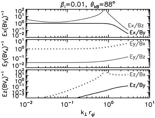
Figure 5. Ratios of the electric field to the fluctuating magnetic field for various combinations.

FIGURE 6

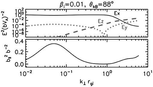
Figure 6. Ratios of the electric field energy to the total magnetic field fluctuation energy (top) and parallel magnetic field energy relative to the total magnetic field fluctuation energy (bottom).

The ratio of E_y to δB_y is also of great interest because the both field components are the leading ones in the kinetic domain. Using the induction equation (Equation 49) and the diamagnetic current type magnetic field polarization (Equation 37), the ratio E_y/δB_y (with normalization to the Alfvén speed) is obtained as

\begin{array}{l} \frac{1}{V_{A}} \frac{E_{y}}{δ B_{y}} = \frac{E_{y}}{δ B_{x}} \frac{δ B_{x}}{δ B_{y}} & (59) \end{array}

\begin{array}{l} ≃ - i \frac{3}{2} \frac{v_{th, i}^{2}}{V_{A}^{2}} \frac{k_{‖} V_{A}}{Ω_{i}} (\frac{3}{4} + \frac{T_{e}}{T_{i}}) {(\frac{T_{e}}{T_{i}})}^{- 1} . & (60) \end{array}

By introducing tan θ = k_⊥/k_‖, the squared ratio of Equation (60) is obtained as

\begin{array}{l} \frac{1}{V_{A}^{2}} | \frac{E_{y}}{δ B_{y}} |^{2} = \frac{9}{4} \frac{v_{th, i}^{2}}{V_{A}^{2}} \frac{1}{{tan}^{2} θ} k_{⊥}^{2} r_{gi}^{2} {(\frac{3}{4} + \frac{T_{e}}{T_{i}})}^{2} {(\frac{T_{e}}{T_{i}})}^{- 2} . & (61) \end{array}

Equation (61) indicates that the E_y energy spectrum is flatter than the δB_y spectrum by $k_{‖}^{2} = k_{⊥}^{2} / {tan}^{2} θ$ (see section 2.3).

2.2.6. Density Fluctuation

The species-wise density fluctuation can be computed through the continuity equation, $ω δ n_{s} + n_{0, s} \vec{k} \cdot {\vec{u}}_{s} = 0$ , where the flow velocity ${\vec{u}}_{s}$ is associated with the wave electric field through the current density, ${\vec{j}}_{s} = q_{s} n_{s} {\vec{u}}_{s}$ , and Ohm's law, ${\vec{j}}_{s} = σ_{s} \vec{E}$ as follows (cf., Gary [43]),

\begin{array}{l} {\vec{u}}_{s} = - i ω ϵ_{0} \frac{1}{q_{s} n_{s}} (ϵ_{s} - I) \vec{E} . & (62) \end{array}

Note that the conductivity is related to the dielectric tensor through σ_s = − iωϵ₀(ϵ_s − I). The density fluctuation is linearly proportional to the electric field (through the tensor operation). To obtain the squared density fluctuation in an independent way from the electric field, one may normalize the density fluctuation to the parallel magnetic field fluctuation,

\begin{array}{l} \frac{〈 δ n_{s}^{2} 〉}{n_{0, s}^{2}} \frac{B_{0}^{2}}{〈 δ B_{‖}^{2} 〉} = \frac{Ω_{s}^{2}}{ω_{ps}^{4}} \frac{1}{〈 δ B_{‖}^{2} 〉} | \vec{k} \cdot (ϵ_{s} - I) \vec{E} |^{2} & (63) \end{array}

\begin{array}{l} = \frac{Ω_{s}^{2}}{ω_{ps}^{4}} \frac{ω^{2}}{k_{x}^{2}} \frac{| \vec{k} \cdot (ϵ_{s} - I) \vec{E} |^{2}}{E_{y}^{2}} . & (64) \end{array}

The ion compressibility is contributed largely by E_x since the parallel electric field is smaller than the perpendicular one, E_z ≪ E_x, and the ion compressibility is approximated to

\begin{array}{l} \frac{〈 δ n_{i}^{2} 〉}{n_{0, i}^{2}} \frac{B_{0}^{2}}{〈 δ B_{‖}^{2} 〉} = \frac{4}{9} \frac{V_{A}^{4}}{v_{th, i}^{4}}, & (65) \end{array}

which essentially agrees with the fluid-derivation except for a factor of $\frac{4}{9}$ . This factor is obtained by expressing the temperature not with the thermal velocity but with the sound speed by replacing 3v_th,i/2 by c_s in Equation (14) in Hollweg [29]. One may extend the expression in Equation 65 by correcting for the ion thermal motion and multiplying a factor of ${(1 - \frac{3}{4} μ_{i})}^{2}$ on the right hand side of Equation (65), which reproduces Equation (22) in Hollweg [29]. The electron compressibility is related to the parallel electric field. The leading term is k_z(ϵ_zz − 1)E_z, yielding the electron compressibility in the same form as Equation (65).

The relation of density fluctuation to the E_x component is

\begin{array}{l} \frac{δ n_{i}}{n_{0, i}} = - i \frac{k_{⊥} V_{A}}{Ω_{i}} \frac{E_{x}}{V_{A} B_{0}} = i \frac{V_{A}^{2}}{c^{2}} \frac{d_{i}}{λ_{De}} \frac{1}{k_{‖} λ_{De}} \frac{E_{z}}{V_{A} B_{0}}, & (66) \end{array}

where we introduced the ion inertial length d_i = V_A/Ω_i and used Equation (34). Equation (66) holds for the electrons, too.

2.3. Spectral Signature

The analytic expressions for the kinetic Alfvén mode properties are useful in interpreting results from observations and numerical simulations for kinetic Alfvén turbulence by, e.g., Howes et al. [9], Passot et al. [10]), Franci et al. [13], Told et al. [15], Valentini et al. [19]. Cerri et al. [23], Grošelj et al. [26]). Perrone et al. [21], and Cerri et al. [27]. In some limited cases, the analytic expressions are also useful to estimate the energy spectra for the kinetic Alfvén mode, assuming the turbulent field is primarily composed of linear-mode waves. The ratio of fluctuation energies of the electric field ( $| E_{x} |^{2}$ , $| E_{y} |^{2}$ , $| E_{z} |^{2}$ ) to that of the total magnetic field fluctuation ( $| δ B_{total} |^{2} = | δ B_{x} |^{2} + | δ B_{y} |^{2} + δ B_{z} |^{2}$ ) (Figure 6) indicate that the x and z components of electric field can be expressed by a scaling law. The x component of electric field to the magnetic field fluctuation is, with the help of Equation (29), written as:

\begin{array}{l} \frac{| E_{x} |^{2}}{| δ B_{total} |^{2}} ≃ \frac{| E_{x} |^{2}}{| δ B_{y} |^{2}} & (67) \end{array}

\begin{array}{l} \propto {\begin{matrix} V_{A}^{2} & (k_{⊥} r_{gi} < 1) \\ (\frac{3}{4} + \frac{T_{e}}{T_{i}}) V_{A}^{2} k_{⊥}^{- 2} r_{gi}^{- 2} & (k_{⊥} r_{gi} ~ 1) \end{matrix} & (68) \end{array}

The y component of electric field becomes larger than x at even higher wavenumbers, and the energy ratio to the magnetic field is (using Equation 61)

\begin{array}{l} \frac{| E_{y} |^{2}}{| δ B_{total} |^{2}} ≃ \frac{| E_{y} |^{2}}{| δ B_{y} |^{2}} & (69) \end{array}

\begin{array}{l} \propto \frac{v_{th, i}^{2} k_{⊥}^{2} r_{gi}^{2}}{{tan}^{2} θ} (k_{⊥} r_{gi} > 1) . & (70) \end{array}

The z component using Equations (29) and (31) as:

\begin{array}{l} \frac{| E_{z} |^{2}}{| δ B_{total} |^{2}} ≃ \frac{| E_{z} |^{2}}{| δ B_{y} |^{2}} & (71) \end{array}

\begin{array}{l} \propto {\begin{matrix} {(\frac{T_{e}}{T_{i}})}^{2} V_{A}^{2} k_{‖}^{2} k_{⊥}^{2} r_{gi}^{4} & (k_{⊥} r_{gi} < 1) \\ (\frac{3}{4} + \frac{T_{e}}{T_{i}}) V_{A}^{2} k_{‖}^{2} r_{gi}^{2} & (k_{⊥} r_{gi} > 1) \end{matrix} & (72) \end{array}

Different scenarios are possible to assess k_‖ in the scaling law:

1. Filamentation. A parallel-propagating Alfvén wave interacts with a density perturbation in the perpendicular plane to the mean magnetic field and the wave-wave interaction generates daughter waves which propagate in highly oblique directions to the mean field. If the density perturbation has a vanishing parallel wavenumber, the daughter waves retain the parallel wavenumber of the pump Alfvén wave (e.g., [45]). In the filamentation scenario, the parallel wavenumber is a constant,

\begin{array}{l} k_{‖} = const . & (73) \end{array}

2. Constant propagation angle. Multi-spacecraft observations indicate that the treatment of constant propagation angle over a wider range of wavenumbers is a valid assumption for dominant wave components in the solar wind [39, 40].

\begin{array}{l} k_{‖} = \frac{k_{⊥}}{tan θ} . & (74) \end{array}

3. Critical balance. The energy transfer time is modeled as scale-wise balanced between the eddy turnover time in the perpendicular plane to the mean magnetic field $τ_{ed} = {(k_{⊥} u_{⊥})}^{- 1}$ (which originates in the fluid non-linearity) and the Alfvén time scattering time $τ_{A} = {(k_{‖} V_{A})}^{- 1}$ along the mean magnetic field (which originates in the hydromagnetic non-linearity):

\begin{array}{l} k_{⊥} u_{⊥} ~ k_{‖} V_{A} . & (75) \end{array}

The flow velocity in the perpendicular plane is assumed to follow the Richardson-Kolmogorov scaling:

\begin{array}{l} u_{⊥} ~ k_{⊥}^{- 1 / 3} ϵ_{turb}^{1 / 3}, & (76) \end{array}

where ϵ_turb denotes the energy transfer rate in the inertial range of fluid turbulence, and is modeled as the flow kinetic energy (proportional to the square of flow velocity, $u_{⊥}^{2}$ ) divided by eddy turnover time ${(k_{⊥} u_{⊥})}^{- 1}$ . Combination of Equation (75) with Equation (76) yields a relation between the parallel and perpendicular components of wavevector:

\begin{array}{l} k_{‖} ~ k_{⊥}^{2 / 3} L^{1 / 3}, & (77) \end{array}

where $L = V_{A}^{3} / ϵ$ is a integration-scale length of the system [42].

Figure 7 displays sketches of the energy spectra deduced from our dielectric tensor method, in particular, using the fluctuation energy ratios shown in Figure 6. We assume a Kolmogorov-type spectral slope −5/3 at lower wavenumbers (MHD inertial range) and an electron-MHD-type spectral slope −7/3 at higher wavenumbers (dispersive range) as presented in the theoretical studies [34, 36] as well as in the hybrid Vlasov-Maxwell numerical study [16]. The small-scale spectrum may be even steeper than −7/3. For example, a hybrid simulation study by Franci et al. [13] presents a steepening of the spectral curve from −5/3 in the MHD domain to −3 in the kinetic domain while a flattening of the electric field spectrum to a slope of −2/3 or −1 and a steepening of magnetic field spectrum (steeper than −7/3) are found in the kinetic range by hybrid simulations by Servidio et al. [14], Cerri and Califano [46], Cerri et al. [20], and Arzamasskiey et al. [47]. The observational values of the short-wavelength slope are, e.g., −2.1 [2], −2.5 [48], and −2.6 [49].

FIGURE 7

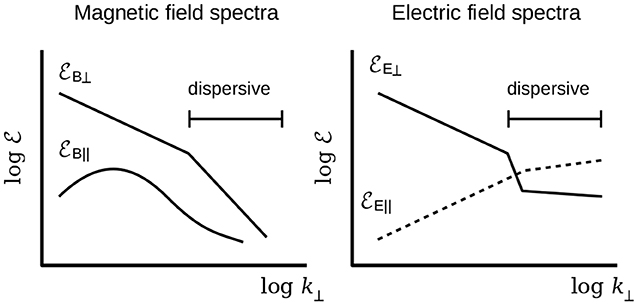
Figure 7. Schematic energy spectra for the magnetic field (left) and electric field (right) of the kinetic Alfvén mode in the perpendicular wavenumber domain.

The perpendicular electric field spectrum falls with the same slope as the magnetic field energy at lower wavenumbers, and falls more steeply than the magnetic field spectrum by a slope difference −2. Yet, at sufficiently high wavenumbers (higher than the wavenumber for the ion gyro-radius), the perpendicular electric field spectrum exhibits a flattening because the out-of-plane component (E_y component) becomes more significant than the in-plane component (E_x component). The perpendicular electric field spectrum has a slope of −1/3 for the constant propagation angle and −1 for the critical balance (assuming that the magnetic field spectrum has a slope of −7/3). The parallel electric field spectrum exhibits a different sense of the slope because the parallel electric field spectrum increases rapidly toward higher wavenumbers. Three different scenarios above indicate that the slope difference of the parallel electric field spectrum to the magnetic field spectrum is 2 (filamentation), 4 (constant propagation angle), and 10/3 (critical balance) at lower wavenumbers, and 0 (filamentation), 2 (constant propagation angle), and 4/3 (critical balance). Yet, it should be noted that the Landau damping parallel to the mean magnetic field is not included in our discussion. The dominance of parallel electric field energy depends on several details of the system under consideration, e.g., injection amplitude and separation of scales. The parallel magnetic field does not exhibit a simple scaling to the perpendicular magnetic field. The parallel field becomes enhanced at wavelengths around the ion inertial length and the ion gyro-radius.

From polarization (or transport ratio) point-of-view, the steepening of perpendicular electric field spectrum occurs because E_x fluctuation energy (in-plane component in a nearly electrostatic sense) becomes smaller than the total magnetic field fluctuation energy at shorter wavelengths around the ion gyro-radius. Then E_y (out-of-plane component in a nearly electromagnetic sense) becomes increasingly larger at even shorter wavelengths and the E_y leads to a flattening of perpendicular electric field spectrum. Figure 5 shows the competition between E_x and E_y components in terms of fluctuation amplitudes, and Figure 6 the competition in terms of the fluctuation energies. A drop of perpendicular electric field spectral curve at wavelengths close to ion gyro-radius has, so far, not been clearly identified in the numerical simulation studies or observations. Possible explanations include effects of higher-order correction of the wave properties (through dielectric response) to thermal and kinetic effects and excitation of other fluctuation modes (e.g., linear-mode waves, forced waves by wave-wave interactions, non-linear mode) that mediate energy cascade of kinetic Alfvén turbulence. Component-wise transport ratio studies will help to diagnose the realization of kinetic Alfvén mode in turbulent kinetic plasmas in the observational and simulation studies.

Our naive estimate of spectral signature for kinetic Alfvén turbulence predicts a local minimum of parallel magnetic field spectrum at wavelengths close to the thermal ion gyroradius. This is because the electric field changes the rotation sense of wave field. Hybrid and particle-in-cell simulations [27] show an evidence for a local minimum of the spectral slope in the energy spectrum of parallel magnetic field in the perpendicular wavenumber domain (but not changing the sign of spectral slope). Note that Figure 7 merely reflects the fluctuation sense studies presented in Figure 6 on the assumption of two distinct power-law spectral domains for the perpendicular magnetic field fluctuations. Yet, increasing sense of the parallel magnetic field fluctuation and flattening of the perpendicular electric field spectrum (relative to the perpendicular fluctuation) are presented in numerical studies by Told et al. [15]. The parallel electric field spectrum often exhibits a decaying sense of spectral curve toward higher wavenumbers (e.g., [21]). Growing sense of the spectrum (with a positive value of spectral index) is confirmed at lower wavenumbers in the Eulerian hybrid Vlasov-Maxwell simulations but not in the hybrid particle-in-cell simulations [22]. The parallel magnetic field spectrum has the nearly same spectral curve to the perpendicular magnetic field spectrum, and has a smaller energy density than the perpendicular magnetic field spectrum (e.g., [21]). The perpendicular electric field spectrum has a larger energy density than the parallel electric field spectrum, and the spectral curve is flatter than the parallel spectrum in the kinetic domain (e.g., [21]). Flattening of the perpendicular electric field spectrum agrees with the hybrid simulation [13, 14, 20, 46, 47], gyro-kinetic simulation [9], fluid-model simulation [10], and particle-in-cell simulation [26].

3. Lessons and Outlook

Analytic derivation of the kinetic Alfvén mode properties is presented in the lowest order picture (which reproduces the transport ratios of the wave in the fluid picture) by assessing the dielectric response in various directions, such as the polarization drift, Debye screening, and Hall and diamagnetic currents and evaluating the transport ratios directly by evaluating the dielectric tensor. The presented method has a wide range of applications in the sense that the dielectric tensor method offers an algorithm to perform higher-order thermal corrections due to the finite Larmor radius and Alfvén wave couplings with the fast and ion-acoustic mode (e.g., treating ϵ_xz as a non-zero quantity).

The dielectric tensor method shows that the Hall and diamagnetic currents contribute to the wave properties through the off-diagonal dielectric response. The off-diagonal dielectric response determines the polarization property of the kinetic Alfvén mode without altering the dispersion relation significantly.

The (temporal) rotation of electric field is in the electron gyration sense, right-hand polarized when viewing into the mean magnetic field direction at a fixed point in space. The field rotation sense originates in the diamagnetic current in the wave. Field rotation sense may be reversed when the Hall current dominates in the (off-diagonal) dielectric response, particularly when the perpendicular wavenumber is not sufficiently large.

The obtained analytic expressions are simplified by using approximations, and then are tested against the transport ratios obtained numerically from the dielectric tensor in Equations (2)–(7). From a practical point of view, Equations (18), (21), (30), (31), (36), (45) provide useful tools of fluctuation sense studies, which can easily be implemented for various data analyses and applications to further studies.

The analytic expression of the transport ratios will serve as a useful tool in the spacecraft observations of wave phenomena, e.g., electric and magnetic field fluctuations in the inner heliospheric region by Parker Solar Probe, Solar Orbiter, and BepiColombo. Even though the measurements are limited to the magnetic field fluctuations only (e.g., the BepiColombo MPO spacecraft measures the interplanetary magnetic field during its 7-years cruise to Mercury) the dielectric tensor method offers a reference model of transport ratios for the kinetic Alfvén mode.

Of course, there could be other modes (both linear and non-linear modes) contributing to the sub-ion-scale fluctuations in solar wind turbulence, which may then show different behavior of the spectral ratios (e.g., [16, 24, 34]) and cause deviations from the expected kinetic Alfvén mode ratios (e.g., [27]). Numerical simulations would play an important role to identify the linear and non-linear modes when the kinetic Alfvén mode evolves into turbulence and to properly associate the transport ratios with various wave modes.

Our study is based on the linear-mode wave properties, in which fluctuation amplitudes are assumed to be sufficiently lower than the mean magnetic field and the waves do not interact with one another (otherwise wave-wave interactions can in general produce forced or pumped waves that differ from the linear mode of the system. Under what condition the mean magnetic field may be treated as a homogeneous and time-stationary field will be an important question when working on the spacecraft data In the case of strong turbulence, fluid non-linearities (eddies and coherent structures) play a more important role.

Author Contributions

YN worked on the calculations and manuscript writing. OR, ZV, and MH worked on the discussion of the wave properties and finalization of the manuscript.

Funding

The work by YN was financially supported by the Austrian Space Applications Programme (ASAP) at the Austrian Research Promotion Agency under contract 853994 and 865967. YN also acknowledges financial support by the Japan Society for the Promotion of Science, Invitational Fellowship for Research in Japan (Long-term) under grant FY2019 L19527. The work by ZV was supported by the Austrian Science Fund (FWF) project P28764-N27.

Conflict of Interest

The authors declare that the research was conducted in the absence of any commercial or financial relationships that could be construed as a potential conflict of interest.

Acknowledgments

YN thanks the research and administration staff members of the Hoshino laboratory group at the University of Tokyo for discussions, supports, and organizations during the fellowship program and the University of Tokyo Mejirodai International Village for the arrangement and hospitality during the pleasant and productive stay in Tokyo.

References

1. Hasegawa A, Uberoi C. The Alfvén Wave. Oak Ridge, TN: Tech. Inf. Center, US Dept. of Energy (1982).

2. Bale SD, Kellogg PJ, Mozer FS, Horbury TS, Rème H. Measurement of the electric fluctuation spectrum of magnetohydrodynamic turbulence. Phys Rev Lett. (2005) 94:215002. doi: 10.1103/PhysRevLett.94.215002

PubMed Abstract | CrossRef Full Text | Google Scholar

3. Sahraoui F, Goldstein ML, Belmont G, Canu P, Rezeau L. Three dimensional anisotropic k spectra of turbulence at subproton scales in the solar wind. Phys Rev Lett. (2010) 105:131101. doi: 10.1103/PhysRevLett.105.131101

PubMed Abstract | CrossRef Full Text | Google Scholar

4. Salem CS, Howes GG, Sundkvist D, Bale SD, Chaston CC, Chen CHK, et al. Identification of kinetic Alfvén wave turbulence in the solar wind. Astrophys J Lett. (2012) 745:L9. doi: 10.1088/2041-8205/745/1/L9

PERSPECTIVE article

Transport Ratios of the Kinetic Alfvén Mode in Space Plasmas

1. Introduction

2. Dielectric Response Framework

2.1. Dielectric Tensor

2.2. Transport Ratios

2.2.1. Electric Field Polarization

2.2.2. Parallel Electric Field

2.2.3. Magnetic Field Polarization

2.2.4. Parallel Magnetic Field

2.2.5. E–B Ratios

2.2.6. Density Fluctuation

2.3. Spectral Signature

3. Lessons and Outlook

Author Contributions

Funding

Conflict of Interest

Acknowledgments

References

Appendix A: Polarization, Hall, and Diamagnetic Currents

Appendix B: Dielectric Tensor Calculations

This article is part of the Research Topic

People also looked at