State Tagging for Improved Earth and Environmental Data Quality Assurance

Introduction

Long-term datasets are ubiquitous in many areas of environmental research as they form the foundation against which hypotheses can be tested, emerging trends determined and future scenarios projected. More importantly, it allows investigation of processes whose effects can only be identified over long periods of time and for revealing new questions which could not have been anticipated at the time the monitoring began (Burt, 1994). International programs such as LTER-Europe (Mollenhauer et al., 2018) and GLEON (Hanson et al., 2018), as well as the increasing use of remote sensing data (Scholefield et al., 2016; Rowland et al., 2017), sensor data (e.g., Evans et al., 2016; Horsburgh et al., 2019) and citizen science projects (e.g., Pescott et al., 2015; Brereton et al., 2018) has greatly increased the diversity of volume of environmental data and offers exciting new opportunities (Reis et al., 2015). It has become standard practice, and for some data centres and publications compulsory, to associate these datasets with helpful metadata and many of these would have passed some quality assurance/quality control (QA/QC) procedure prior to publication. An overview of the current practice of data management and QA/QC procedures of environmental data can be found in the volume edited by Recknagel and Michener (2018).

The global proliferation of earth and environmental datasets opens new avenues for discovery (Savage, 2018). The growing number and advances in instruments on land and sea, in the air and in space, alongside with ever-increasing computation capability to produce more detailed model outputs, have generated huge amounts of Earth and environmental science data. However, such a large amount of data from diverse sources makes categorizing and sharing the information difficult. Questions about their quality may prevent them from being reused by other researchers. It has been argued recently that research data should be ‘findable, accessible, interoperable, and reusable’ (FAIR) (Wilkinson et al., 2016; Stall et al., 2019). To this end, many countries have taken bold steps, such as changing journal and funding guidelines to enforce the deposition of data into dedicated repositories and adopting standard procedures for metadata and standard vocabularies. However, current work still largely assumes the user will first download the data, go through some analysis, and then decide whether the dataset is useful. The user has no idea about the data quality and contextual information (and thus whether they can reuse it) until they download the datasets and compare it with some other auxiliary datasets they find elsewhere. As highlighted by a recent review, data quality (or constraining data uncertainty) and methods to choose reliable data for analysis are among the top challenges in environmental data science (Gibert et al., 2018). Some universal tools to give the user a quick idea about the data quality and contextual information of datasets are urgently needed.

For users wanting to make use of long-term monitoring datasets maintained by a third party, data quality is crucial in determining its relevance, while meta-data is important to aid data discoverability and understanding its context. These monitoring schemes are usually managed under a database management system (DBMS) (e.g., Figure 1), where centralized data collection and validation by a coordination unit responsible for the establishment of rules for data transfer and checking routines are recommended. Database managers usually have implemented numerous standard operating procedures and controls to minimize errors in the data sets. Some datasets have quality flags associated with each measurement. Table 1 shows the data quality control system used by the UK Environmental Change Network (ECN) as an example. Such checks mostly handle missing values and check whether the values are within accepted ranges, whilst more advanced checks remove outliers and verify instrumentation calibrations. Sometimes, these checks are refined based on on-site historical data or seasonality.

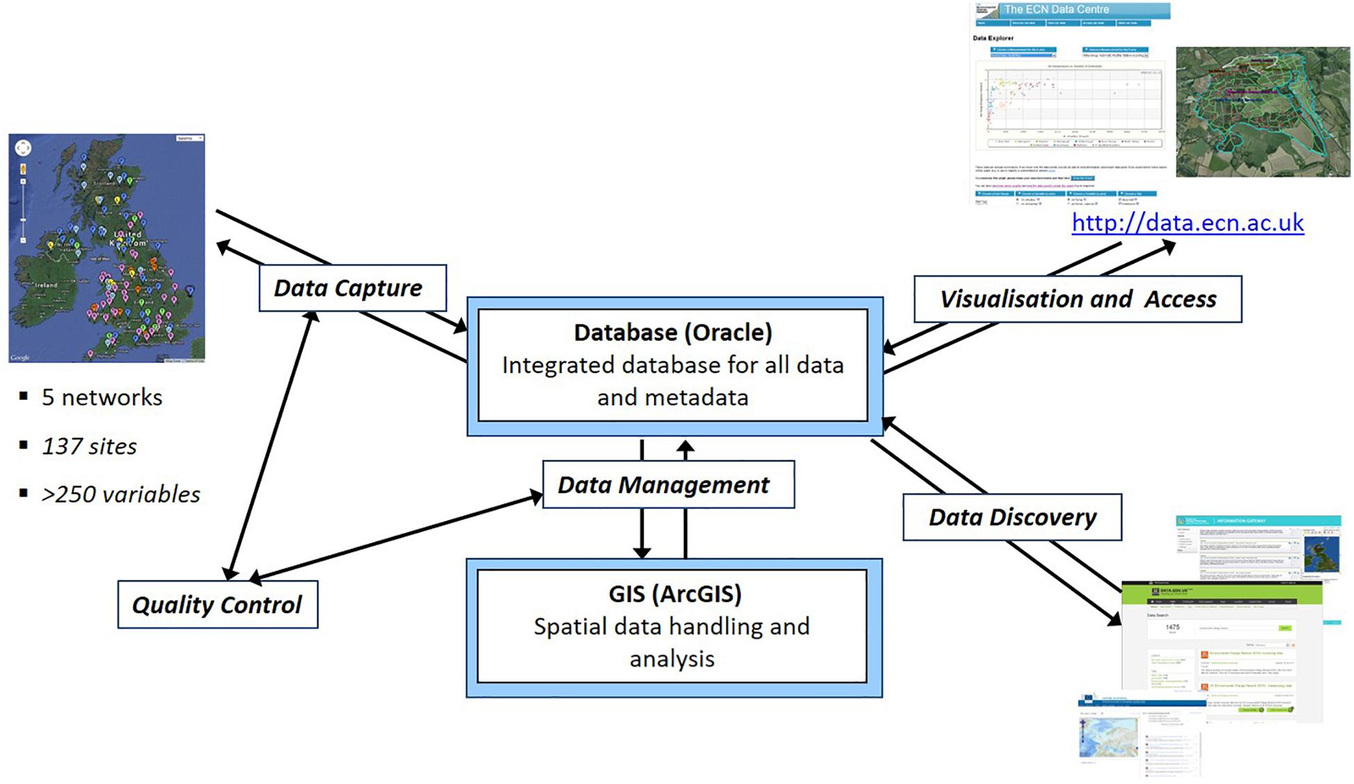
Figure 1. Overview of the ECN Data Centre Information System (Rennie, 2016).

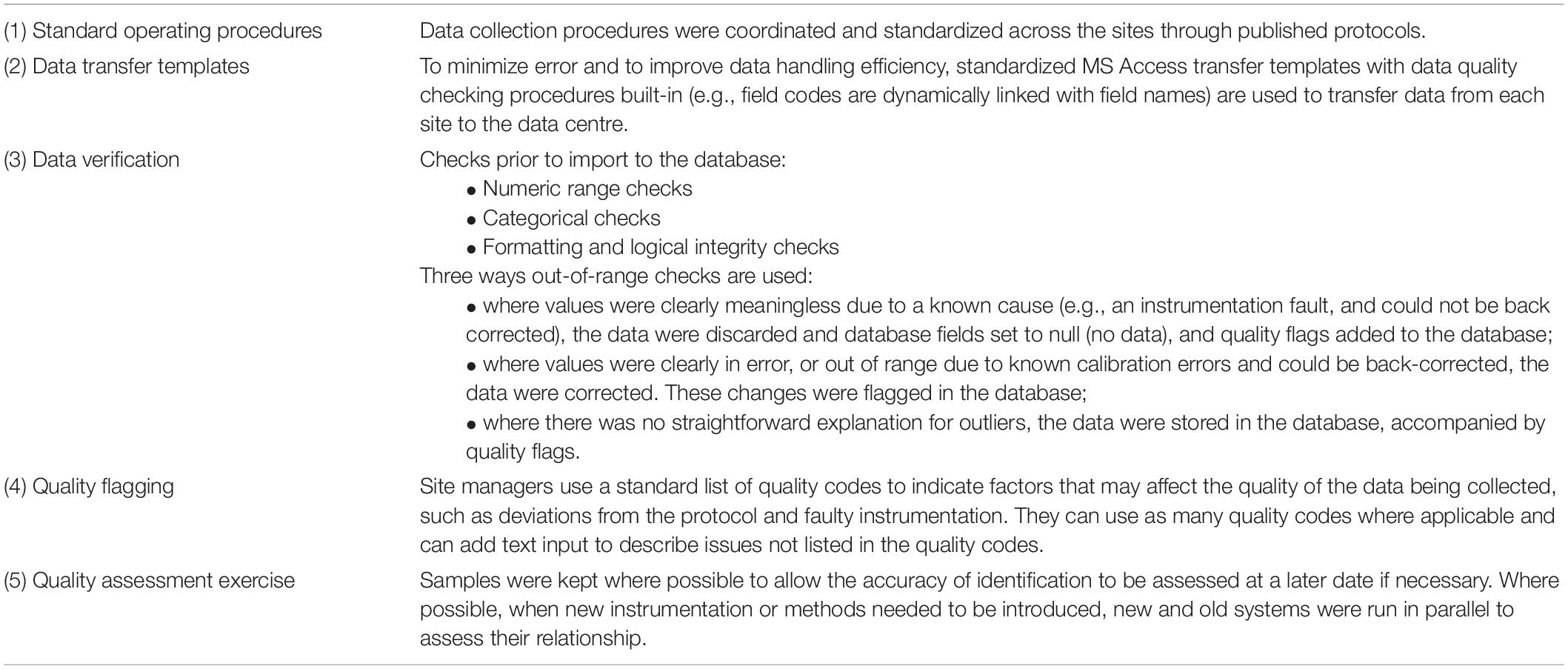
Table 1. An example of data quality control at all stages of data management and collection from ECN (Rennie et al., 1993–2015).

Previous work has discussed the application of quality assurance procedures in large long-term monitoring databases in areas such as forest management (Houston and Hiederer, 2009) and forest monitoring (Ferretti and Fischer, 2013), hydrological and water quality sensor data (Horsburgh et al., 2011, 2015), and streaming ecological sensor networks (Campbell et al., 2013). A relevant procedure is to perform outlier detection and remediation, preferably in a multivariate manner, which has been developed for geochemical databases (Lalor and Zhang, 2001). Strategies have also been developed to detect and control biases between datasets from examining their metadata in chemical soil monitoring (Desaules, 2012a,b).

The quality checks that are adopted currently, although very useful in flagging obvious errors, may be quite broad and limited in utility in terms of providing context on the condition where the measurement is made. For example, moth counts are expected to be low in February, but if a high moth count is observed is this erroneous or is it due to an unusually warm and dry winter? We propose the use of data science techniques to tag each measurement with an identified system state. The term “state” here is defined loosely and represents some aspect of the conditions, be they environmental, procedural or observational, at the time the observation was made. They are identified using multivariate unsupervised classification methods, such as k-means clustering. Once the states are identified, state-dependent prediction intervals can be calculated for each observational variable, thus providing credible ranges conditional on the context defined by the system state. This approach makes range checks account for the system states and, although we still see the user has an important role to play in defining such anomalies, it provides the user with more contextual information to resolve out-of-range flags. In the use cases presented here, ecological experts were consulted on the results from the analyses and in all cases found this method provided helpful contextual information to understand data anomalies. Specifically, the methods can reliably determine whether an anomaly is an outlier or is normal behavior within that state. Therefore, it allows the user to focus on using their expert judgment to test hypotheses. Our method is intended to be a very efficient method that is generic enough to apply to many different types of environmental datasets, such that it may be available, for example, for preview in the download page of a dataset. The use of the state tagging approach does not prevent users from performing more sophisticated analysis subsequently.

This paper describes an approach for system state tagging for long-term monitoring datasets, which is implemented in a virtual environment as part of an analysis workflow pipeline. We demonstrate our approach using two use cases that utilize datasets from the UK Environmental Change Network (ECN) and UK CEH Cumbrian Lakes monitoring scheme. Limitations and future work of this state tagging work are discussed. An R Shiny application (Chang et al., 2015) that allows the user to upload data files and download with the associated states and its source code is made publicly available.

Materials and Methods

Our approach to anomaly detection is based on assessing observations conditional on the context in which they were observed. To do this we wish to define a set of states that reflect any such context and within which we can detect any outliers. Therefore, our approach to anomaly detection uses additional information that we know about the system at the time of the observations – we term this additional information the state variables. In this section, we describe the method adopted for defining states and identifying outliers and the details of its implementation as an R Shiny application.

Unsupervised Classification for State Tagging

The goal of the state tagging task is to associate each observation of the data frame, which is assumed to represent a single value for a single time point at a single spatial location, with one of the defined states. In machine learning, the task to assign data into distinct, discrete categories is considered as a classification task. In the absence of any prior information relating to the states, which is assumed here, an unsupervised classification algorithm is needed. K-means clustering is a computationally efficient unsupervised classification algorithm that has been used extensively in a number of anomaly detection applications, such as network traffic (Münz et al., 2007), environmental risk zoning (Shi and Zeng, 2014), and hotspots of fire occurrences (Suci and Sitanggang, 2016), among many others. The approach has been extended to consider both numerical and categorical data (Huang, 1998) and therefore provides an effective approach for defining states. The standard approach is to perform clustering on a set of multivariate data and the clustering algorithm seeks to find a set of clusters that minimize within cluster variability whilst maximizing between cluster variability. This optimisation is constrained either by a specified number of clusters or by the level of residual variation. In the case of K-means clustering, the variability is defined by the distance between each data point and its cluster center. If the distance exceeds a certain user-defined threshold, the data point can be flagged as an outlier. We used K-means clustering in this paper to illustrate the state tagging concept as it provides a fast and efficient method of state classification with intuitive understanding for users. As a method for initial assessment of potentially high throughput data, this seemed an appropriate approach to take. Alternative unsupervised classification methods could be used instead of K-means clustering and these are compared in Table 2. A comparison of various unsupervised clustering-based classification methods, listing relative strengths and limitations. Other methods also exist for data quality assessment or anomaly detection, although they tend to be application-specific. For example, a 10-step framework is proposed for automated anomaly detection in high-frequency water quality data (Leigh et al., 2019). Similarly, a Dynamic Bayesian Network (DBN) framework is proposed to produce probabilistic quality assessments and represent the uncertainty of sequentially correlated sensor readings for temperature and conductivity sensors (Smith et al., 2012), while association rule learning has been used to detect unusual soil moisture probe response in green infrastructure by taking advantage of the similarity of paired change event (Yu et al., 2018).

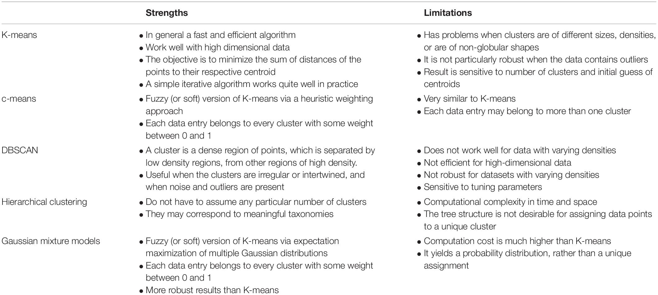
Table 2. A comparison of various unsupervised clustering-based classification methods.

Our approach considers time series data only, where the observation data is a single value for a single point in time for a single spatial location and is available at multiple points in time. As we consider outliers conditional on their state (i.e., conditional on the context at time of recording), our state tagging method requires both state variables and observational variables. Here we define “state variables” as variables that are used for clustering and state definition and hence provide the context of the observation at time of recording, whereas “observational data” are data variables which we wish to attach prediction intervals for quality control purposes. Examples of state variables include meteorological data (e.g., air/water temperature, rainfall, solar radiation, wind speed, relative humidity), detection data (e.g., data that may influence detectability of observations such as time of day, time since last maintenance of sensor, position of sensor) and procedural data (e.g., equipment used, lab method, precision of measurement, sample support) each of which should ideally be available at the same temporal resolution as the observed data. Running a K means clustering algorithm enables classification of each vector of state variables, and hence the aligned observation data, into one of N states, where N is determined a priori. For each observational variable, the data is grouped by the states so that the mean and standard deviation for each observational variable within each state can be calculated. This, in turn, enables calculation of envelopes corresponding to the 68, 95, or 99.5% prediction intervals (which corresponds to mean ± 1, 2, 3 standard deviations) for each measurement. It is then from these intervals that outliers can be classified and are therefore dependent on the wider context in which the observation was made – the state. An overview of the state tagging approach is shown in Figure 2.

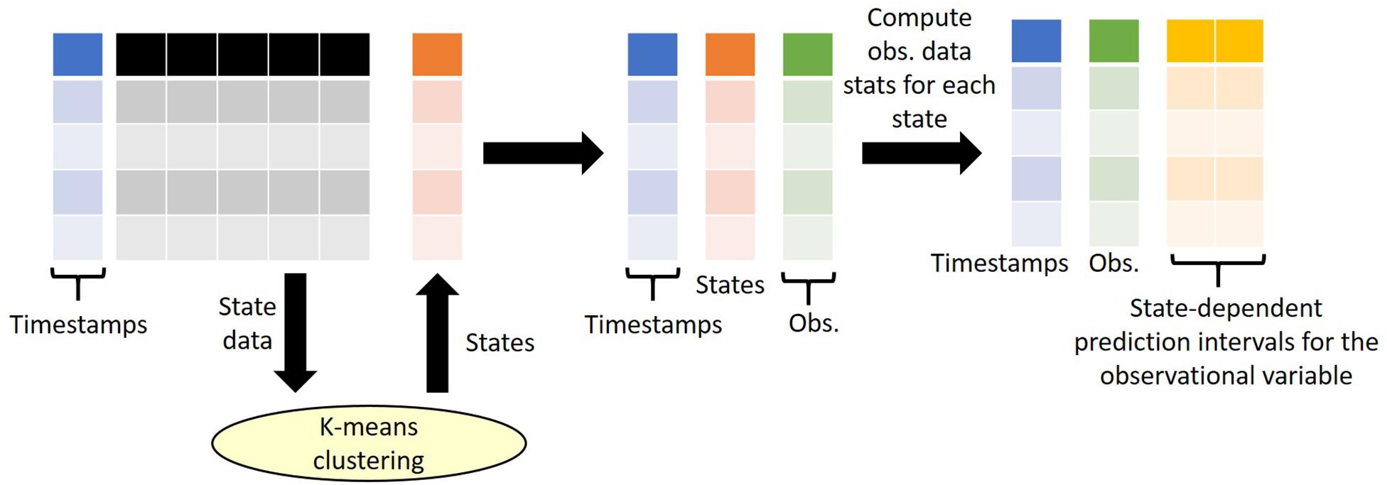
Figure 2. An overview of the state tagging approach. K-means clustering is performed on a selected number of state variables and returns a state number for each row of state data. Note that during the clustering, the timestamps are not considered. Once the states are defined, the states are then attached to the observational data based on matching timestamps (e.g., date). Finally, the statistics of the observational data for each state are computed to derive state-dependent prediction intervals. Observations that fall outside of the prediction intervals are flagged out-of-range.

Implementation as an R Shiny Application

Our state tagging method is implemented as an R Shiny (Chang et al., 2015) application (see Data Availability Statement), which allows user interaction and web hosting on a virtual laboratory environment (see section “Introduction”). The R Shiny framework is highly efficient for creating graphical user interfaces (GUI) and it allows access to many tools (e.g., statistics, machine learning, and plotting) and application programming interfaces (API) relevant to retrieving environmental data that are available in R (Slater et al., 2019). Both R and Python are the most used languages in data science and they have both been used for data visualization and quality control of environmental data (Horsburgh and Reeder, 2014; Horsburgh et al., 2015).

The states are defined by performing k-means clustering using the base R package “stats” on the selected state variables. The data is scaled before clustering. An elbow method, which plots the number of clusters versus data misfit, can be used to determine the optimal number of clusters and avoid over-fitting. Plots are generated to allow interactive visualization of cluster distribution, both as a time series and box and whisker plot of a state variable using the “plotly” framework (Sievert, 2019). Since clustering does not take into account the temporal signature of the state variables, confusion matrix-type plots (i.e., occurrence of state at time t vs. t-1) can be used to assess the temporal behavior of the derived states. Once the states are defined, observational data are associated (or tagged) with the state and prediction interval for the time period (e.g., day, hour). Any data outside of the envelope are flagged.

While we have developed customized versions for the use cases reported here, we make a generalized version of the application available, which allows the user to upload a data file and select state and observational variables from the list of field names available. The R Shiny can accept data in the following formats:

(1) Panel data. The dataset will have a column for date or both date and time. The remaining columns are data values and the column names are field names. NaNs are ignored.

(2) One observation per line. The columns “DATE,” “FIELDNAME,” and “VALUE” are read while other columns are ignored, where “FIELDNAME” is the variable being observed and “VALUE” is the corresponding data value.

Use Cases

We demonstrate the use of the proposed state tagging approach for environmental data using two long-term monitoring datasets in the United Kingdom.

ECN Moth and Butterfly Data

Data

Launched in 1992, ECN collects a broad range of high-frequency environmental data. It includes 12 terrestrial sites that are broadly representative of the environmental conditions in the United Kingdom. These measurements are made in close proximity at each site, using standard protocols incorporating standard quality control procedures (Sykes and Lane, 1996) and great effort has been put to maintain methodology consistency (Beard et al., 1999). ECN data are managed by its dedicated data centre (Rennie, 2016) and can be downloaded from the NERC Environmental Information Data Centre. Protocol documents and supporting documentation are provided alongside the data download. Site managers can assign quality codes to indicate factors that may affect the quality of the data. They can either choose codes from a list of common problems or enter customized texts. These quality data are available within the data download. The informatics approach of the ECN data centre is described in Rennie (2016). ECN is the UK node in a global system of long-term, integrated environmental research networks and is a member of LTER-Europe (the European Long-Term Ecosystem Research Network¹) and ILTER (International Long Term Ecological Research²). Here, we focus the application of our state tagging approach using meteorological, moth, and butterfly data at the ECN site in Wytham, which is encompassed by a loop of the River Thames, 5 km northwest of Oxford. The data used in this section is obtained from the UK Environmental Change Network³ (Rennie et al., 1993–2015).

Light traps are used at ECN sites to sample moths daily (Rennie et al., 2017b). A count of each species trapped is recorded. Butterfly species were recorded on a fixed transect (which was divided into a maximum of 15 sections) (Rennie et al., 2017a). At each site, a co-located weather station is installed to collect hourly weather data (Rennie et al., 2017c). ECN moth and butterfly data have been used in a number of studies, such as developing ecological indicators (i.e., community temperature response, CTR) to predict the phenology response to warming (Martay et al., 2016).

State Tagging

In this example, we have selected four variables: air temperature; rainfall; solar radiation; and wind speed to represent the state variables, all of which are available at daily resolution (specifically, daily mean of hourly observations). The state, therefore, defines the climatological or weather-related context when the measurement was made. The “elbow” curve or L curve, which balances misfit minimisation and avoidance of overfitting of the classification technique, identify the optimal number of clusters to be five. The clustering identifies the five states without supervision. As observed in Figures 3, 4, each of the identified states has distinctive characteristics that describe the system state. A summary of the characteristics of each state is summarized in Table 3. Note that our interpretation here is for illustration purposes only and subject experts may interpret the system states differently. Most days in the time series are represented by states 1, 3, 4, 5, while state 2 represents rainy days (rainfall > 0.2 mm). State 5 represents windy days, while state 3 represents clear, sunny days of high solar radiation. The t vs. (t+1) matrix is helpful to visualize the stability of the states and their potential correlation. For states 1, 3, and 4, there is a probability of more than 70% for the next day to remain in the same state, while that for state 5 is around 50%. Interestingly, there is only a 12% chance for state 2 to remain in the same state, suggesting the system does not tend to have high rainfall (>0.5 mm) for more than a day.

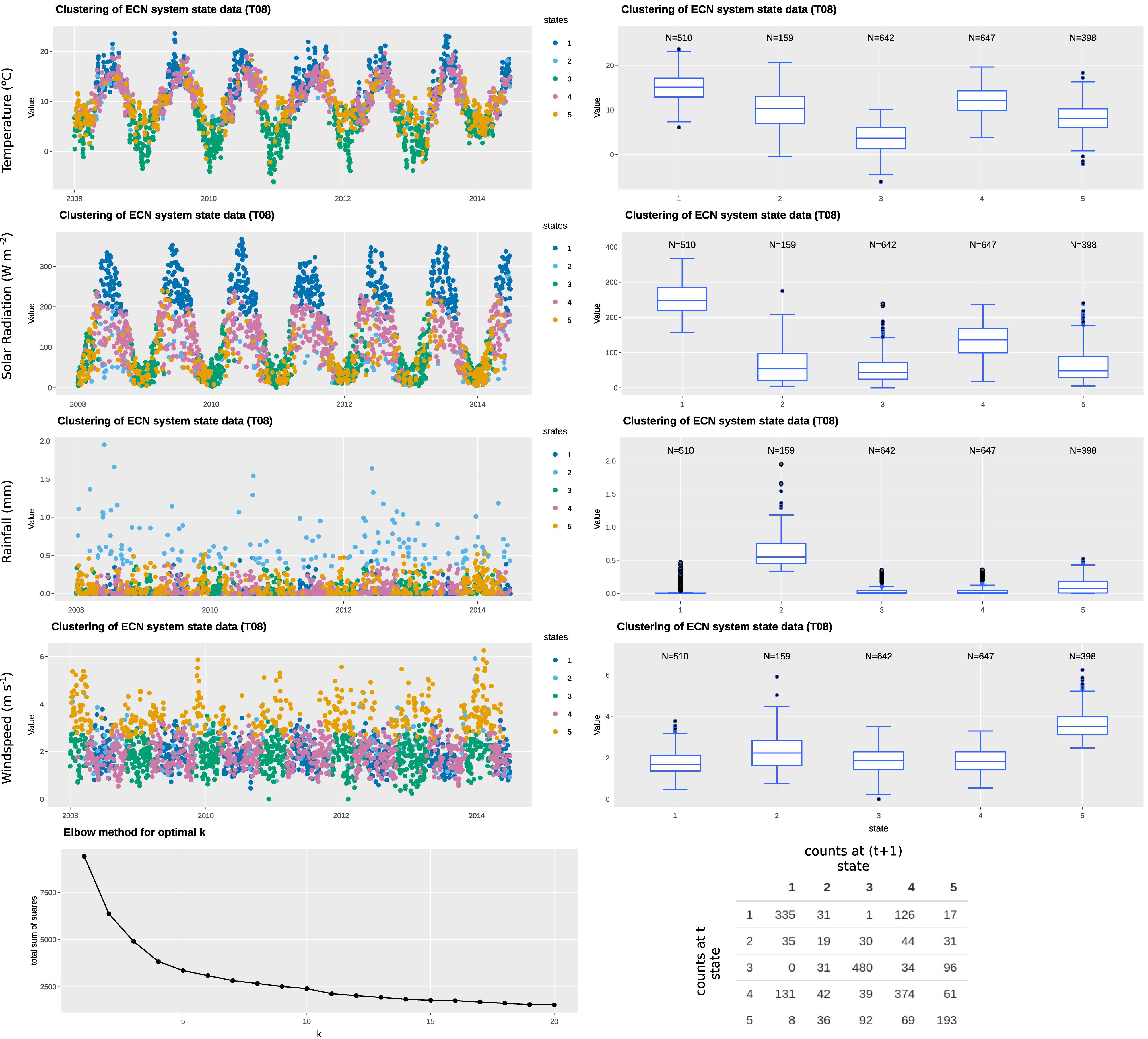
Figure 3. Example of state tagging at the ECN site at Wytham. A box-and-whisker plot is linked to the time series and shows the statistics of the selected state variable for each cluster. An elbow plot is useful to optimize the number of clusters used and avoid overfitting. A t vs. (t+1) matrix is useful to explore the autocorrelation of clusters.

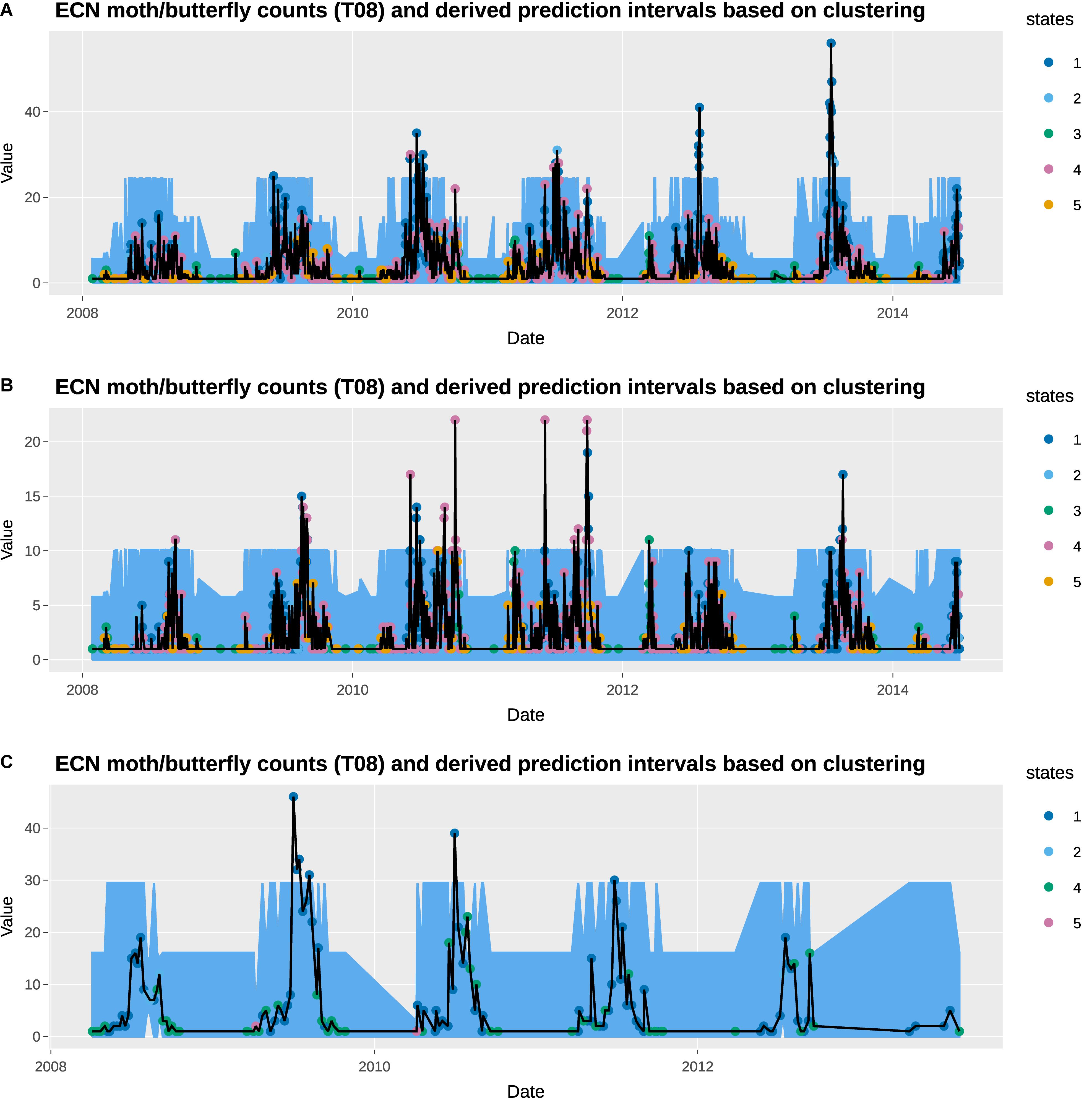
Figure 4. Observed total counts and 95% prediction intervals at Wytham: (A) total moths, (B) total Noctuidae (a moth group), and (C) total butterflies.

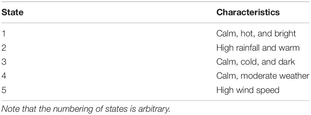
Table 3. Characteristics of the derived state in the example at Wytham.

Prediction Intervals

The empirical prediction intervals obtained from the observation data within consistent states are overlaid on the observed moths and butterflies data, which are also available at daily resolution. The observed data shows high seasonal variability, with high moth counts in the summer, and high butterfly counts in the spring. In general, the prediction intervals capture the general seasonal variability very well. In particular, the change in states captures the increase in moth counts in the summer months. However, the observed moth counts in those moths tend to be much greater than the upper prediction interval, suggesting the 95% threshold used here may be too low. None of the prediction intervals gives a daily total moth count that exceeds 27. A higher threshold, such as 99.5% can be used instead. This is obviously a subjective choice of the user and hence why deploying the method within the R Shiny application has significant benefits.

States 3 and 5 are generally associated with low moth counts days, and all the observations fall within the prediction intervals. States 1 and 4 are associated with the days with the highest and third-highest moth counts, which appears to have a prediction interval that is too narrow. Interestingly, state 2 has the second-highest prediction intervals, although its upper interval for total moth counts is only 17.8. We observe similar trends in the Noctuidae data. One notable difference is that state 4 is associated with the highest Noctuidae counts instead of state 1.

Most butterfly data are recorded on either a state 1 or state 4 day, with the former denoting a high butterfly count day. Under the ECN protocol adopted from the UK Butterfly Monitoring Scheme, butterfly data is only recorded between the 1^st April and 29^th September on days satisfying the following conditions. Sampling took place when the temperature was between 13 and 17°C if sunshine was at least 60%; but if the temperature was above 17°C (15°C at more northerly sites) recording could be carried out in any conditions, providing it was not raining. They generally capture the highs and lows of butterfly counts, but as with the moth data, the high observed butterfly counts are significantly above the prediction intervals. States 2 and 5 only have one or two butterfly counts data points (none of the days with butterfly data available is tagged with state 3), which result in the very narrow prediction intervals.

UK Lake Ecosystem Data

Data

Data from the UK CEH Cumbrian Lakes monitoring scheme is retrieved for this use case. It consists of automatic water monitoring buoy data (Jones and Feuchtmayr, 2017) and long-term manual sampling data (Maberly et al., 2017). The automatic lake monitoring buoy carries a range of meteorological instruments and in-lake temperature sensors. These instruments make measurements every 4 min, with hourly averages provided in the dataset. Data are available from 2008 to 2011. The long-term manual sampling data were collected fortnightly from 1945 to 2013. Surface temperature, surface oxygen, water chemistry, water clarity and phytoplankton chlorophyll a data were collected. We focus our analysis on the data collected at Blelham Tarn, a small lake in the U.K.’s Lake District, from 2008 to 2011.

State Tagging

In this example, we have selected three variables: water temperature; solar radiation; and wind speed as state variables from the automatic monitoring buoy data, all of which are available at hourly resolution. We have aggregated the data to daily resolution for state tagging to match the resolution of the observation variable and to even out any daily effects. The “elbow” curve or L curve, which balances misfit minimisation and avoidance of overfitting, identify the optimal number of clusters to be four. The clustering identifies the four states without supervision. As observed in Figures 5, 6, each of the identified states has distinctive characteristics that describe the system state. A summary of the characteristics of each state is summarized in Table 4. Note that our interpretation here is for illustration purposes and subject experts can interpret the system states differently. States 2 and 4 represent fewer days than others do, possibly because they represent more extreme weather (i.e., warm/high solar radiation and high wind speed, respectively). As observed in the Box-and-whisker plots, long-tail clusters exist for some states. For example, the distribution of solar radiation in states 1 and 4 are highly skewed. This is typical for some meteorological variables such as solar radiation and wind speed, which tend to skew toward zero and are sometimes modeled by zero-inflated models. The t vs. (t+1) matrix is helpful to visualize the stability of states. If we broadly define states 2 and 3 is the main group for warmer months and states 1 and 4 for cooler months, we can see that there are many occurrences where the system fluctuates between within-group states. However, there are also about 10–20 occurrences per year where the system switches from one group to another. Further investigation on these days is of interest because they represent the system is not in a state where it is normally associated with at that time of the year (e.g., windy days in 2008).

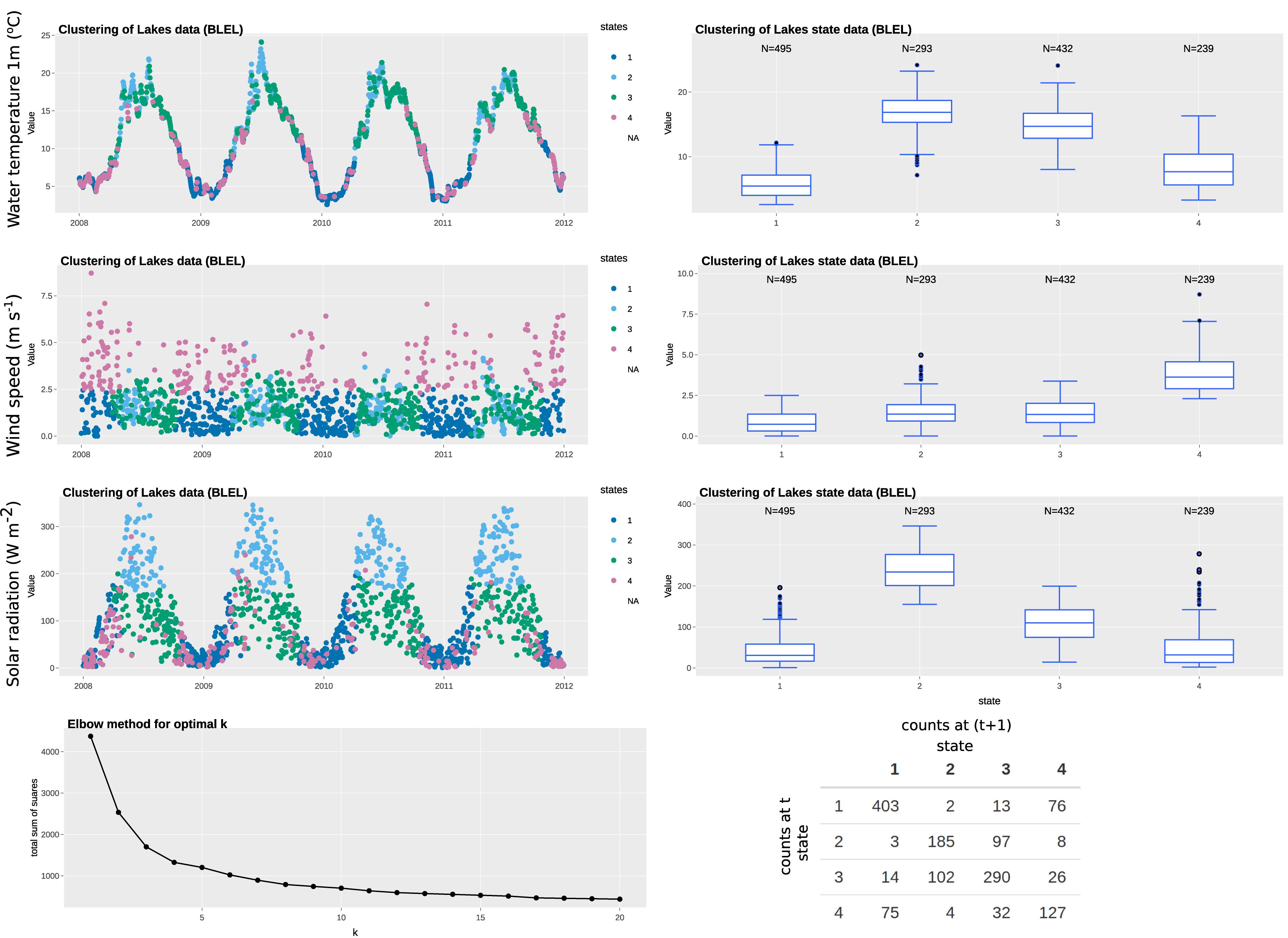
Figure 5. Example of state tagging at the lake ecosystems site of Blelham Tarn. A box-and-whisker plot is linked to the time series and shows the statistics of the selected state variable for each cluster. An elbow plot is useful to optimize the number of clusters used and avoid overfitting. A t vs. (t+1) matrix is useful to explore the autocorrelation of clusters.

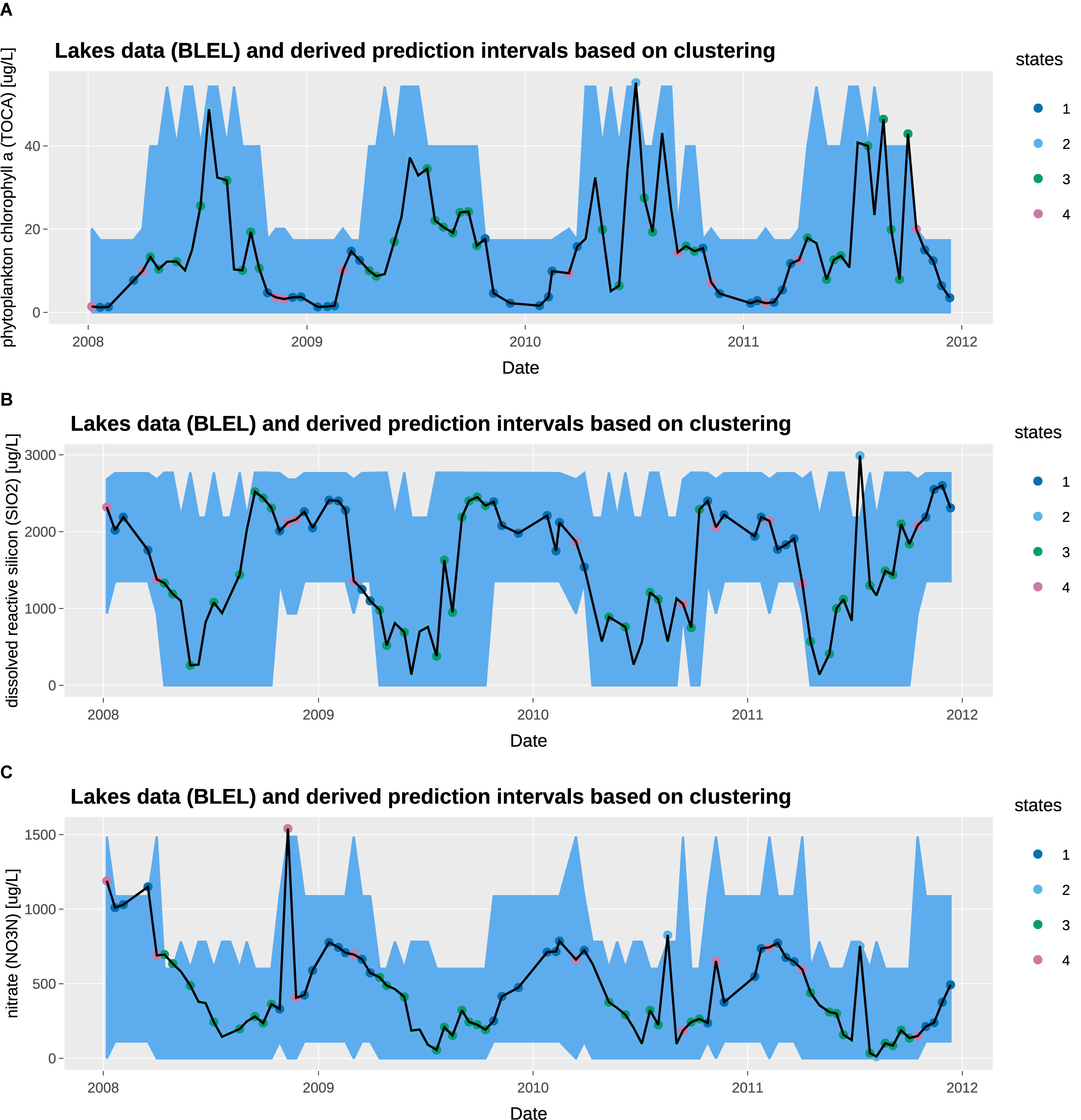
Figure 6. Observed concentration and 95% prediction intervals at Blelham Tarn: (A) total chlorophyll a [μg/L], (B) dissolved reactive silicon [μg/L], (C) nitrate [μg/L].

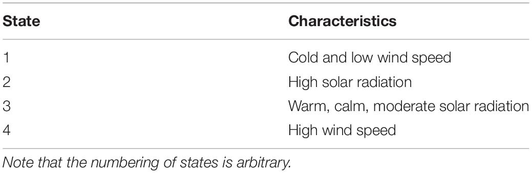
Table 4. Characteristics of the derived state in the example at Blelham Tarn.

Prediction Intervals

We overlay the prediction intervals obtained from state tagging on the observed water chemistry data. The observed data shows high seasonal variability, with high chlorophyll a, low nitrate and low dissolved reactive silicon in the summer; and the inverse in the winter. In general, the prediction intervals capture the high seasonal variability very well. From a QC/QA perspective, the 95% threshold capture most of the observations with only a few exceptions. The prediction intervals for states 1 and 4 are similar, capturing generally the low chlorophyll a, high dissolved reactive silicon, and high nitrate in winter months. Similarly, the prediction intervals for states 2 and 3 are similar, capturing the high chlorophyll a, low dissolved reactive silicon, and low nitrate in summer months. However, state 2 shows a wider prediction interval, which can be attributed to the high solar radiation on clear summer days.

As discussed in the state tagging section, it is possible for states to fluctuate over short periods of time. However, ecological observations may take some time to respond to changes in system state or they represent the averaged system state over a period of time. In these cases, the user may decide to introduce a time lag in the state tagging stage, or averaging the state variables over a rolling time window.

Discussion

Benefits for Users and Managers of Environmental Data

Providing information on quality control is a key requirement for providers and users of environmental data. It allows users to determine whether they can trust a data resource, particularly when they have no contact with the data originators. For a programme like ECN, this state tagging approach should provide a step-change in its ability to provide quality information. Until now ECN quality checking has involved a number of range checks (Rennie et al., 1993–2015) that are usually applied within each protocol. It is worth mentioning that the ECN data used in this paper has already passed range checks before clustering. So any data points outside the prediction interval are anomalies not detected previously. Using state tagging will provide contextual information for the quality flags that are applied – giving confidence to users and enabling them to make more informed decisions when using the data.

It should also improve the efficiency with which the data can be quality checked. State tagging will help differentiate between data that are unusual but can be explained given the contextual information, and those data that are problematic and require greater scrutiny from data managers. The ECN datasets are extensive and cover multiple domains, and therefore quality checking is a time-consuming exercise. Using this state tagging approach to target data that need more detailed quality checking should prove a time saver and improve the quality of data that are made available. We emphasize that the meaning of the states identified by the unsupervised state tagging method is arbitrary and they do not involve specialist interpretation.

Lessons Learned

K-means clustering is an unsupervised machine learning method so the states identified are arbitrary and the clustering result can differ with different record length, the variability of the state variables captured, and the number of clusters. Since the numbering of states is arbitrary and is assigned at random, the random seed is fixed in the shiny app for reproducible results. State variables (especially meteorology data) are commonly available at many monitoring sites or nearby weather stations in hourly resolution. Since most observation variables are recorded at daily or lower resolution and the goal of clustering is to capture primary variability in the state variables, it is sensible to aggregate the sub-daily state variables to daily values before clustering and to tag each day with a state, i.e., the resolution of the state variables should match the resolution of the observation variables. Clustering is computationally very efficient and our approach is suitable for the four “Vs” of Big data (volume, velocity, variety, veracity) because it can handle a large amount of highly variable data at a high speed and produces useful prediction intervals. To accelerate the method, the clustering can be applied to a subset of the state data and apply to the entire dataset (e.g., training using only 5 years out of the 20+ years of ECN data).

Our choice of clustering for state tagging has advantages over black-box artificial intelligence (AI) algorithms, namely the cluster centers and spread can be easily interpretable and its computation time is negligible even for large datasets. However, deep learning can be used for more specific prediction tasks. The state variables used for clustering is not limited to meteorological or chemical variables—they can also be other information related to how the measurement is made. For example, identifiers for the equipment or personnel used can be included. In general, one should use system understanding to guide the choice of variables that are used in clustering, such that the defined states are relevant to the observational variables to which prediction intervals are attached.

Currently, the state tagging method is used as a QA/QC tool. However, it can potentially be used as a tool to identify phenomena of interest. For example, if a researcher is only interested in warm, wet winter, the state tagging approach can identify the states and only a subset of dataset tagged with the state of interest is retrieved. Alternatively, the state tagging approach can be trained using existing data and used in forecasting future observations. Specifically, future data can be tagged to a state defined by pre-existing data and associate observations with prediction intervals. The t vs. (t+1) confusion matrix can be used to predict empirically the probability for the next day to be associated with the various states (sum = 1.0), which in turn can be used as weights for prediction intervals in forecasts.

Limitation of K-Means Clustering

Our clustering-based state tagging method takes no consideration of time. Therefore, the system may fluctuate between two states. Our method has the potential to be reformulated to determine whether there is an abrupt change of system state. For instance, changepoints detection methods (Killick et al., 2012) can be used to identify jumps in the time series. State tagging efforts will benefit from recent advances in multivariate changepoints detection (Bardwell et al., 2019).

Contribution to the Data Science Framework

Clustering is only applicable to rows of data where all fields are available (otherwise, an NA state is returned). This is not an issue if the state variables are meteorological variables obtained from automatic weather stations where measurements are synchronized. However, if other variables are used for state tagging, the measurements may not be synchronized. A nearest-neighbor search may be needed to align measurements taken within a certain time range to the same data entry. Alternatively, gap-filling approaches can be used to fill in missing data, especially for datasets that have large gaps. An approach to accelerate the FAIR use of datasets and models is through the use of online collaborative research platform. Such platforms ensure data, information and forecasting capabilities are accessible, timely and efficient. Since datasets can be easily accessed from within the platform, assessing the quality of datasets using auxiliary datasets can be seamlessly achieved. The state tagging approach fits nicely to the many research initiatives explores the concept of virtual data labs (Blair et al., 2018), which are online collaborative facilities to bring together a wide range of software tools, multiscale simulations and observations, and teams with different levels of technical skills. Since data from these virtual data labs are from a wide variety of data sources, it will be useful to have state tagging tools available so that users do not have to look for the system state elsewhere. Prediction intervals provide contextual information in addition to range checks for users to assess the quality and reliability of data. Such a framework should be applied widely to virtual data labs and it should be implemented in different levels of abstraction, from using the default setup described here to allowing users to customize their state tagging routine in the data.

Future Work

It has been argued recently that the use of machine-learning approaches in the earth and environmental sciences should not simply amend classical machine learning approaches. Rather, contextual cues should be used as part of deep learning to gain further process understanding (Reichstein et al., 2019). The state tagging method contributes to extracting these contextual cues at the data quality assurance stage. Recently, deep learning has also been used to fill gaps in long-term monitoring records (Ren et al., 2019). Future work should consider extending the proposed state tagging approach to gap-filled datasets. Likewise, although methods exist for real-time Bayesian anomaly detection in streaming environmental data (Hill et al., 2009; Hill, 2013), they do not currently account for other contextual information. Using both state tagging and real-time anomaly detection can ensure greatest reliability of environmental data. For live data feeds, we do not recommend reanalyzing the entire dataset whenever new data are received. Instead, the new data should decide whether a new measurement belongs to one of the existing clusters, or a new cluster should be created. At the moment, prediction intervals based on states are calculated for a single variable at a time. Future work should consider prediction for multivariate data. For example, consistency checks for flags for various variables at the same time point can be performed. Finally, our work assumes the data are from traditional sensors or manual sampling. Latest developments in intelligent sensor and internet of things (IoT) (Nundloll et al., 2019) allows sensors to be equipped with its own QA/QC, while mark-up languages for metadata of environmental data have been developed to improve their interoperability (Horsburgh et al., 2008). These advances offer exciting opportunities to expand the idea of state tagging for environmental data.

Conclusion

A clustering-based state tagging framework has been developed for improved quality assurance of long-term earth and environmental data. The proposed approach is highly flexible and efficient that it can be applied to a large volume of virtually any point data in environmental monitoring. It serves as a way to provide additional contextual information for quality assurance of environmental data. Importantly, it will give greater confidence to users and enable them to make more informed decisions when using the data. Such functionality is particularly relevant to virtual research platforms that are linked to a vast number of datasets (e.g., to various data centres) as they provide infrastructure support to facilitate complex, collaborative research in the earth and environmental sciences (Blair et al., 2018) and tackle environmental data science challenges (Blair et al., 2019).

Data Availability Statement

The source code of the R Shiny application for system state tagging (generic version) is available at the NERC Environmental Information Data Centre (EIDC): https://doi.org/10.5285/1de712d3-081e-4b44-b880-b6a1ebf9fcd8 (Tso, 2020). It can be run in any platforms with R and required R packages installed. Users can upload the data file of their choice.

Readers may interact with the customized versions of the R Shiny application for the UK ECN and Cumbrian lakes data, which are currently hosted at the following URLs:

ECN moth and butterfly state tagging app: https://statetag-ecnmoth.datalabs.ceh.ac.uk/.

Lakes state tagging app: https://statetag-lakes.datalabs.ceh.ac.uk/.

Generic version (including source code): https://statetag-generic.datalabs.ceh.ac.uk/.

The datasets analyzed are freely available from the NERC Environmental Information Data Centre (EIDC) under the terms of the Open Government License using the following DOI’s:

ECN data

Butterflies: https://doi.org/10.5285/5aeda581-b4f2-4e51-b1a6-890b6b3403a3 (Rennie et al., 2017a).

Moths: https://doi.org/10.5285/a2a49f47-49b3-46da-a434-bb22e524c5d2 (Rennie et al., 2017b).

UK CEH Cumbrian Lakes monitoring scheme data (Blelham Tarn)

Automatic buoy: https://doi.org/10.5285/38f382d6-e39e-4e6d-9951-1f5aa04a1a8c (Jones and Feuchtmayr, 2017).

Long-term manual sampling data: https://doi.org/10.5285/393a5946-8a22-4350-80f3-a60d753beb00 (Maberly et al., 2017).

Author Contributions

C-HT wrote the manuscript and developed the methods and the R Shiny applications that implement the approach. JW and PH designed the research. SR wrote the manuscript. All co-authors contributed to the editing, discussion, and review of this manuscript.

Funding

This work was part of the UK-SCAPE: UK Status, Change and Projections of the Environment project, a National Capability award funded by the UK Natural Environmental Research Council (NERC: NE/R016429/1). Additional funding was provided by the Data Science of the Natural Environment project awarded to Lancaster University and CEH (EPSRC: EP/R01860X/1).

Conflict of Interest

The authors declare that the research was conducted in the absence of any commercial or financial relationships that could be construed as a potential conflict of interest.

Acknowledgments

We thank Don Monteith, Heidrun Feuchtmayr, and Stephen Thackeray at UKCEH for discussions on the ECN and Cumbrian lakes data. We thank Mike Hollaway and Iain Walmsley for assistance in deploying the R Shiny apps on DataLabs. We would like to acknowledge our colleagues in the Centre of Excellence in Environmental Data Science (CEEDS), a collaboration between Lancaster University and the UK Centre for Ecology & Hydrology.

Footnotes

1. ^ http://www.lter-europe.net/
2. ^ http://www.ilternet.edu/
3. ^ http://www.ecn.ac.uk

References

Bardwell, L., Fearnhead, P., Eckley, I. A., Smith, S., and Spott, M. (2019). Most recent changepoint detection in panel data. Technometrics 61, 88–98. doi: 10.1080/00401706.2018.1438926
Beard, G. R., Scott, W. A., and Adamson, J. K. (1999). The value of consistent methodology in long-term environmental monitoring. Environ. Monit. Assess. 54, 239–258. doi: 10.1023/A:1005917929050
Blair, G. S., Henrys, P., Leeson, A., Watkins, J., Eastoe, E., Jarvis, S., et al. (2019). “Data science of the natural environment: a research roadmap,” in CMWR Conference (Computational Methods in Water Resources, St Malo. doi: 10.3389/fenvs.2019.00121
Blair, G. S., Watkins, J., August, T., Bassett, R., Brown, M., Ciar, D., et al. (2018). Virtual Data Labs: Technological Support for Complex, Collaborative Research in the Environmental Sciences. Available online at: https://www.ensembleprojects.org/wp-content/uploads/2018/04/Virtual -Labs-2-pager-actual-format-FINAL.pdf (accessed January 1, 2020).
Brereton, T. M., Botham, M. S., Middlebrook, I., Randle, Z., Noble, D., Harris, S., et al. (2018). United Kingdom Butterfly Monitoring Scheme Report for 2017. Available online at: http://www.ukbms.org/reportsandpublications.aspx (accessed January 1, 2020).
Burt, T. P. (1994). Long-term study of the natural environment - perceptive science or mindless monitoring? Prog. Phys. Geogr. Earth Environ. 18, 475–496. doi: 10.1177/030913339401800401
Campbell, J. L., Rustad, L. E., Porter, J. H., Taylor, J. R., Dereszynski, E. W., Shanley, J. B., et al. (2013). Quantity is nothing without quality: automated QA/QC for streaming environmental sensor data. Bioscience 63, 574–585. doi: 10.1525/bio.2013.63.7.10
Chang, W., Cheng, J., Allaire, J., and Xie, Y. (2015). Shiny: Web Application Framework for R. Available online at: https://shiny.rstudio.com/ (accessed January 1, 2020).
Desaules, A. (2012a). Measurement instability and temporal bias in chemical soil monitoring: sources and control measures. Environ. Monit. Assess. 184, 487–502. doi: 10.1007/s10661-011-1982-1
Desaules, A. (2012b). The role of metadata and strategies to detect and control temporal data bias in environmental monitoring of soil contamination. Environ. Monit. Assess. 184, 7023–7039. doi: 10.1007/s10661-011-2477-9
Evans, J. G., Ward, H. C., Blake, J. R., Hewitt, E. J., Morrison, R., Fry, M., et al. (2016). Soil water content in southern England derived from a cosmic-ray soil moisture observing system – COSMOS-UK. Hydrol. Process. 30, 4987–4999. doi: 10.1002/hyp.10929
Ferretti, M., and Fischer, R. (eds) (2013). Forest Monitoring – Methods for terrestrial investigations in Europe with an overview of North America and Asia. Amsterdam: Elsevier, doi: 10.1016/B978-0-08-098222-9.00009-1
Gibert, K., Horsburgh, J. S., Athanasiadis, I. N., and Holmes, G. (2018). Environmental data science. Environ. Model. Softw. 106, 4–12. doi: 10.1016/j.envsoft.2018.04.005
Hanson, P. C., Weathers, K. C., Dugan, H. A., and Gries, C. (2018). “The global lake ecological observatory network,” in Ecological Informatics, ed. F. Recknagel (Cham: Springer International Publishing), 415–433. doi: 10.1007/978-3-319-59928-1_19
Hill, D. J. (2013). Automated bayesian quality control of streaming rain gauge data. Environ. Model. Softw. 40, 289–301. doi: 10.1016/j.envsoft.2012.10.006
Hill, D. J., Minsker, B. S., and Amir, E. (2009). Real-time bayesian anomaly detection in streaming environmental data. Water Resour. Res. 45:W00D28. doi: 10.1029/2008WR006956
Horsburgh, J. S., Caraballo, J., Ramírez, M., Aufdenkampe, A. K., Arscott, D. B., and Damiano, S. G. (2019). Low-cost, open-source, and low-power: but what to do with the data? Front. Earth Sci. 7:67. doi: 10.3389/feart.2019.00067
Horsburgh, J. S., and Reeder, S. L. (2014). Data visualization and analysis within a hydrologic information system: integrating with the R statistical computing environment. Environ. Model. Softw. 52, 51–61. doi: 10.1016/j.envsoft.2013.10.016
Horsburgh, J. S., Reeder, S. L., Jones, A. S., and Meline, J. (2015). Open source software for visualization and quality control of continuous hydrologic and water quality sensor data. Environ. Model. Softw. 70, 32–44. doi: 10.1016/j.envsoft.2015.04.002
Horsburgh, J. S., Tarboton, D. G., Maidment, D. R., and Zaslavsky, I. (2008). A relational model for environmental and water resources data. Water Resour. Res. 44:W05406. doi: 10.1029/2007WR006392
Horsburgh, J. S., Tarboton, D. G., Maidment, D. R., and Zaslavsky, I. (2011). Components of an environmental observatory information system. Comput. Geosci. 37, 207–218. doi: 10.1016/j.cageo.2010.07.003
Houston, T. D., and Hiederer, R. (2009). Applying quality assurance procedures to environmental monitoring data: a case study. J. Environ. Monit. 11:774. doi: 10.1039/b818274b
Huang, Z. (1998). Extensions to the k-means algorithm for clustering large data sets with categorical values. Data Min. Knowl. Discov. 2, 283–304. doi: 10.1023/A:1009769707641
Jones, I., and Feuchtmayr, H. (2017). Data from automatic water monitoring buoy from Blelham Tarn, 2008 to 2011. doi: 10.5285/38f382d6-e39e-4e6d-9951-1f5aa04a1a8c
Killick, R., Fearnhead, P., and Eckley, I. A. (2012). Optimal detection of changepoints with a linear computational cost. J. Am. Stat. Assoc. 107, 1590–1598. doi: 10.1080/01621459.2012.737745
Lalor, G. C., and Zhang, C. (2001). Multivariate outlier detection and remediation in geochemical databases. Sci. Total Environ. 281, 99–109. doi: 10.1016/S0048-9697(01)00839-7
Leigh, C., Alsibai, O., Hyndman, R. J., Kandanaarachchi, S., King, O. C., McGree, J. M., et al. (2019). A framework for automated anomaly detection in high frequency water-quality data from in situ sensors. Sci. Total Environ. 664, 885–898. doi: 10.1016/j.scitotenv.2019.02.085
Maberly, S. C., Brierley, B., Carter, H. T., Clarke, M. A., De Ville, M. M., Fletcher, J. M., et al. (2017). Surface Temperature, Surface Oxygen, Water Clarity, Water Chemistry and Phytoplankton Chlorophyll a Data from Blelham Tarn, 1945 to 2013. Bailrigg: Environmental Information Data Centre, doi: 10.5285/393a5946-8a22-4350-80f3-a60d753beb00
Martay, B., Monteith, D. T., Brewer, M. J., Brereton, T., Shortall, C. R., and Pearce-Higgins, J. W. (2016). An indicator highlights seasonal variation in the response of Lepidoptera communities to warming. Ecol. Indic. 68, 126–133. doi: 10.1016/j.ecolind.2016.01.057
Mollenhauer, H., Kasner, M., Haase, P., Peterseil, J., Wohner, C., Frenzel, M., et al. (2018). Long-term environmental monitoring infrastructures in Europe: observations, measurements, scales, and socio-ecological representativeness. Sci. Total Environ. 624, 968–978. doi: 10.1016/j.scitotenv.2017.12.095
Münz, G., Li, S., and Carle, G. (2007). “Traffic anomaly detection using kmeans clustering,” in Proceedings GI/ITG Workshop MMBnet.
Nundloll, V., Porter, B., Blair, G. S., Emmett, B., Cosby, J., Jones, D. L., et al. (2019). The design and deployment of an end-to-end iot infrastructure for the natural environment. Future Internet 11:129. doi: 10.3390/fi11060129
Pescott, O. L., Walker, K. J., Pocock, M. J. O., Jitlal, M., Outhwaite, C. L., Cheffings, C. M., et al. (2015). Ecological monitoring with citizen science: the design and implementation of schemes for recording plants in Britain and Ireland. Biol. J. Linn. Soc. 115, 505–521. doi: 10.1111/bij.12581
Recknagel, F., and Michener, W. K. (2018). Ecological Informatics. Cham: Springer International Publishing, doi: 10.1007/978-3-319-59928-1
Reichstein, M., Camps-Valls, G., Stevens, B., Jung, M., Denzler, J., Carvalhais, N., et al. (2019). Deep learning and process understanding for data-driven Earth system science. Nature 566, 195–204. doi: 10.1038/s41586-019-0912-1
Reis, S., Seto, E., Northcross, A., Quinn, N. W. T., Convertino, M., Jones, R. L., et al. (2015). Integrating modelling and smart sensors for environmental and human health. Environ. Model. Softw. 74, 238–246. doi: 10.1016/j.envsoft.2015.06.003
Ren, H., Cromwell, E., Kravitz, B., and Chen, X. (2019). Using deep learning to fill spatio-temporal data gaps in hydrological monitoring networks. Hydrol. Earth Syst. Sci. Discuss. doi: 10.5194/hess-2019-196
Rennie, S., Adamson, J., Anderson, R., Andrews, C. M., Wood Bater, J., Bayfield, N., et al. (2017a). UK Environmental Change Network (ECN) Butterfly Data: 1993-2015. Bailrigg: Environmental Information Data Centre, doi: 10.5285/5aeda581-b4f2-4e51-b1a6-890b6b3403a3
Rennie, S., Adamson, J., Anderson, R., Wood, C., Bate, J., Bayfield, N., et al. (2017b). UK Environmental Change Network (ECN) Moth Data: 1992-2015. Bailrigg: Environmental Information Data Centre, doi: 10.5285/a2a49f47-49b3-46da-a434-bb22e524c5d2
Rennie, S., Adamson, J. R. A., Andrews, C., Bater, J., Bayfield, N., Beaton, K., et al. (2017c). UK Environmental Change Network (ECN) Meteorology Data: 1991-2015. Bailrigg: Environmental Information Data Centre, doi: 10.5285/fc9bcd1c-e3fc-4c5a-b569-2fe62d40f2f5
Rennie, S., Andrews, C., Atkinson, S., Beaumont, D., Benham, S., Bowmaker, V., et al. (1993–2015). The UK environmental change network datasets – Integrated and co-located data for long-term environmental research (1993–2015). Earth Syst. Sci. Data Discuss. 12, 87–107. doi: 10.5194/essd-2019-74
Rennie, S. C. (2016). Providing information on environmental change: data management, discovery and access in the UK environmental change network data centre. Ecol. Indic. 68, 13–20. doi: 10.1016/j.ecolind.2016.01.060
Rowland, C. S., Morton, R. D., Carrasco, L., McShane, G., O’Neil, A. W., and Wood, C. (2017). Land Cover Map 2015 (1km Percentage Target Class, GB). Bailrigg: Environmental Information Data Centre, doi: 10.5285/505d1e0c-ab60-4a60-b448-68c5bbae403e
Scholefield, P., Morton, D., Rowland, C., Henrys, P., Howard, D., and Norton, L. (2016). A model of the extent and distribution of woody linear features in rural Great Britain. Ecol. Evol. 6, 8893–8902. doi: 10.1002/ece3.2607
Shi, W., and Zeng, W. (2014). Application of k-means clustering to environmental risk zoning of the chemical industrial area. Front. Environ. Sci. Eng. 8:117–127. doi: 10.1007/s11783-013-0581-5
Sievert, C. (2019). Interactive Web-Based Data Visualization with R, Plotly, and Shiny. Available online at: https://plotly-r.com/ (accessed January 1, 2020).
Slater, L. J., Thirel, G., Harrigan, S., Delaigue, O., Hurley, A., Khouakhi, A., et al. (2019). Using R in hydrology: a review of recent developments and future directions. Hydrol. Earth Syst. Sci. 23, 2939–2963. doi: 10.5194/hess-23-29392019
Smith, D., Timms, G., De Souza, P., and D’Este, C. (2012). A bayesian framework for the automated online assessment of sensor data quality. Sensors 12, 9476–9501. doi: 10.3390/s120709476
Stall, S., Yarmey, L., Cutcher-Gershenfeld, J., Hanson, B., Lehnert, K., Nosek, B., et al. (2019). Make scientific data FAIR. Nature 570, 27–29. doi: 10.1038/d41586-019-01720-7
Suci, A. M. Y. A., and Sitanggang, I. S. (2016). Web-based application for outliers detection on hotspot data using k-means algorithm and shiny framework. IOP Conf. Ser. Earth Environ. Sci. 31:012003. doi: 10.1088/1755-1315/31/1/012003
Sykes, J. M., and Lane, A. M. J. eds. (1996). The UK Environmental Change Network: Protocols for Standard Measurements at Terrestrial Sites. London: Stationery Office.
Tso, C.-H. M. (2020). State tagging application for environmental data quality assurance. NERC Environ. Inform. Data Centre. doi: 10.5285/1de712d3-081e-4b44-b880-b6a1ebf9fcd8
Wilkinson, M. D., Dumontier, M., Aalbersberg, J., Appleton, G., Axton, M., Baak, A., et al. (2016). Comment: the FAIR guiding principles for scientific data management and stewardship. Sci. Data 3:160018. doi: 10.1038/sdata.2016.18
Keywords: data science, quality assurance, data analytics, environmental monitoring, environmental informatics, clustering (unsupervised) algorithms
Citation: Tso C-HM, Henrys P, Rennie S and Watkins J (2020) State Tagging for Improved Earth and Environmental Data Quality Assurance. Front. Environ. Sci. 8:46. doi: 10.3389/fenvs.2020.00046
Received: 17 December 2019; Accepted: 06 April 2020;
Published: 06 May 2020.
Edited by:
Peng Liu, Institute of Remote Sensing and Digital Earth (CAS), ChinaReviewed by:
Luis Gomez, University of Las Palmas de Gran Canaria, SpainDavide Moroni, Istituto di Scienza e Tecnologie dell’Informazione “Alessandro Faedo” (ISTI), Italy
Copyright © 2020 Tso, Henrys, Rennie and Watkins. This is an open-access article distributed under the terms of the Creative Commons Attribution License (CC BY). The use, distribution or reproduction in other forums is permitted, provided the original author(s) and the copyright owner(s) are credited and that the original publication in this journal is cited, in accordance with accepted academic practice. No use, distribution or reproduction is permitted which does not comply with these terms.
*Correspondence: Chak-Hau Michael Tso, mtso@ceh.ac.uk