Prediction of Wetland Hydrogeomorphic Type Using Morphometrics and Landscape Characteristics

Introduction

One of the means of categorizing wetlands is according to hydrogeomorphic (HGM) type, which is defined by geomorphic setting (e.g., hillslope or valley-bottom), water source (e.g., surface water dominated or sub-surface water dominated) and pattern of water flow through the wetland unit (diffuse or channeled) (Brinson, 1993; Ollis et al., 2013). Given the fact that HGM types are defined in terms of key driving process that underlie wetlands (Brinson, 1993) they provide a useful means of inferring ecosystem functioning and supply of ecosystem services (Euliss et al., 2013) as well as a means of delimiting broad response units for ecological condition assessments (Kotze et al., 2012). It has been noted further how HGM types differ in terms of degradation patterns (Rivers-Moore and Cowden, 2012) and vulnerabilities (Kotze, 2011). Therefore, classifying wetlands according to HGM type has a potentially useful contribution to make toward assessing and promoting the sustainable use of wetlands, particularly at a broad catchment/landscape scale.

While data on wetland extent, HGM type, and ecological condition are increasingly recognized as important for global- and regional-scale (province, state, county, or catchment) wetland assessments, methods, and studies on these approaches are limited worldwide (Guidugli-Cook et al., 2017). Historically, wetlands have been iteratively mapped and typed using a combination of field assessments and interpretation of aerial photographs. This is not only a labor intensive process, but typically leaves large swathes of landscape under-mapped. Consequently, there is an increasingly widespread application of satellite imagery data for wetland inventory and mapping; although currently used techniques have recognized limitations for detecting some types of wetlands (see for example Davidson et al., 2018). Whereas, national wetland inventories are not available for many parts of the world, where these do exist, there are often concerns about accuracy, or data deficiency such as for cases when wetland polygons have no attributes. Large discrepancies in concurrence between national inventories and field observations of wetlands (Guidugli-Cook et al., 2017) raises concerns about the reliable use of national datasets when scrutinized at a regional or local scale.

In South Africa there are tens of thousands of wetlands covering 2.6 million hectares (van Deventer et al., 2020), and therefore to type all of these wetlands manually would require considerable resources. If reliable automated method/s using model/s can be developed for identifying HGM type, they offer the means of typing wetlands at a fraction of the cost of doing so manually.

However, to date, attempts to automate the identification of HGM type have met with very limited success, and in two test areas in the Western Cape, the automated HGM types yielded a very low level of congruency with the field-verified HGM types (van Deventer et al., 2016). For previous studies on modeling HGM type for South Africa, the analysis was based on a 90 m digital elevation model (DEM) and on the interim step of generating landform classes (van Deventer et al., 2016). While adequate for representing the range of landforms at a country-wide scale, there was an under-estimation of slope and an over-estimation of valley floors, and an overall accuracy of 43% was estimated for prediction of wetland HGM type which is not sufficient for decision making at the local scale (van Deventer et al., 2014). Nevertheless, fundamental to setting conservation targets for landscape features such as wetlands, as well as prioritizing wetland systems, for example, for rehabilitation, is a sound spatial layer of wetland occurrence (location and extent) that includes information on wetland hydrogeomorphic type and ecological condition. Here, we recognize that spatial wetland ancillary data should be developed in a logical sequence, beginning with occurrence and extent, followed by hydrogeomorphic (HGM) type, and then ecological condition. We include ecological condition as the final step based on catchment-scale ecological condition models that showed that different HGM types respond to different predictor variables; for example, elevation was the best predictor of floodplain ecological condition, while population density was a significant predictor of seep ecological condition (Rivers-Moore and Cowden, 2012). Given the variable nature of these wetland parameters within the landscape, it is more pragmatic to assign degrees of probability rather than absolute classifications to mapped wetlands. In other words, ancillary data layers will be able to provide probability values for occurrence, type, and ecological condition, from which wetland practitioners will be able to make statements such as “at this location, there is an 85% probability of a wetland occurring, which is five times more likely to be a seep than a floodplain, and there is a 70% probability that it is in a degraded state.” Here, the ecological condition of a wetland refers to present condition relative to an un-impacted reference condition which shows little or no influence of human actions (Anderson, 1991). In southern Africa, owing to limited availability of data on biological response indicators, the assessment of ecological condition generally requires a strong reliance on stressor-based indicators, in particular relating to land-cover and land-use in the wetland and its influent catchment (Kotze et al., 2012). The assessment method developed by Kotze et al. (2012) provides standardized metrics for assessing ecological condition of wetlands in South Africa, and is designed to account as far as possible for the differential responses of HGM types to specific stressors.

It is therefore logical that landscape-level predictive models, based on “soft” classification techniques, should be used to complement traditional approaches to wetland mapping. In South Africa, logistic regression models in different regions of the country have already indicated that prediction accuracy for both occurrence and ecological condition differ between HGM types (Rivers-Moore and Cowden, 2012; Hiestermann and Rivers-Moore, 2015; Melly et al., 2016). However, in both case studies, these ancillary probability layers were dependent on extensive baseline wetland mapping exercises. The development of such spatial layers requires a complementary process of baseline wetland mapping and predictive model development. Baseline wetland maps provide a testing and verification dataset for model development, while the latter provides ancillary data on wetland occurrence and ecological condition to assist in improving baseline wetland inventories.

For wetland type classifications in South Africa, the Level IV classification (HGM type) by Ollis et al. (2013, 2015) is in standard use by wetland practitioners, and is in line with other global classification systems (Brinson, 1993). The classification of Level IV HGM units, including seep, depression, valley-bottom, and floodplain wetland types, also takes cognizance of inland vs. coastal systems, regional setting, and landscape position. Therefore, there is a great need for the development of refined and more robust models to allow HGM type to be identified more reliably. Here, we develop and test a simple approach for predicting the most likely HGM type for mapped yet unattributed wetland polygons.

Methods

Study Area

Our study area was defined on the basis of having two reliable, adjacent and independent datasets of wetland polygons available (Figure 1). Both datasets describe a range of wetland types in the Western Cape province of South Africa, within the Cape Floristic region. The naturally occurring vegetation in this area is “fynbos” (a distinctive, Mediterranean climate, sclerophyllous vegetation biome only occurring on the southern tip of Africa); despite relatively high levels of land cover transformation, wetland HGM types would be generally unaffected by these changes. This is based on direct observation that climate, geology and landscape position govern occurrence and type (Hiestermann and Rivers-Moore, 2015; Ollis et al., 2015), whereas land cover transformation and degradation underpin ecological condition (Kotze et al., 2012). Underlying geology consists primarily of a mix of sandstones and fractured metasedimentary rock, interspersed with subordinate shales and mudstones; Table Mountain sandstones dominate in the west, while the Cape Fold Mountains fractured metasedimentary rocks occur in the east (Colvin et al., 2007). Topography is highly heterogeneous, with much of the study area characterized by relatively short (50–300 km) rivers in deeply incised valleys.

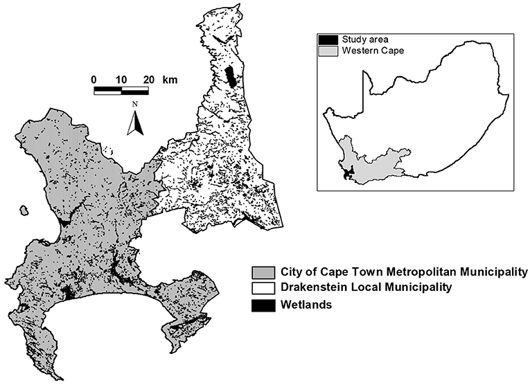
Figure 1. Map of study area, showing City of Cape Town and Drakenstein municipalities and their respective wetlands datasets; inset shows context of study area within the Western Cape Province of South Africa.

Datasets used for this study were the wetlands coverage for the City of Cape Town metropolitan municipality (n = 7,272 polygons; City of Cape Town, 2017), and the Drakenstein local municipality (n = 4,237 polygons; Day et al., 2009). While falling in to the same predominantly winter rainfall region, the two study areas cover a rainfall gradient from relatively wetter in the west to relatively drier in the east (mean annual precipitation gradient of ~600–200 mm; Schulze, 1997), within a Mediterranean climate.

Within the study area, the majority of mapped wetlands have been classified to Level IV HGM type, according to the classification defined by Ollis et al. (2013). Datasets were compiled by wetland specialists, with HGM types assigned through a combination of field assessments and local terrain knowledge.

Analyses

Only inland wetlands were considered, with estuarine HGM types excluded from analyses. The number and area of HGM units per dataset were described using bar and pie charts. HGM polygons for the study area (n = 11,379) were next attributed in terms of their landscape position, shape and likely links to groundwater (Colvin et al., 2007).

• Landscape position included the metrics elevation (90 m digital elevation model; USGS, 2018), from which slope and aspect (both degrees) were derived using appropriate surface analysis algorithms (Clark Labs, 2009). Relief ratio, as an indication of catchment terrain roughness, was also derived from the DEM, using quaternary catchments (fourth order catchments; primary management areas for South Africa, based on a standardized mean annual runoff per unit area; Midgley et al., 1994) as the overlay image, and basin length and change in elevation (maximum minus minimum elevation) for each catchment. Lastly, HGM types were attributed by their association with Strahler stream order and geomorphological zone (upland vs. lowland, based on 1:500,000 scale river longitudinal zones with a breakpoint between upper and lower foothills; Moolman, 2006).

• HGM polygon attributes: Area (m²) and perimeter (m); Log transformation of area and perimeter; shape (area: perimeter ratio—Equation 1); fractal dimension (Equation 2)

• Groundwater depth (m below ground; Colvin et al., 2007).

Wetland HGM data were then screened for differences in the metrics (shape, area, fractal dimension, perimeter: area ratio) between regions using a Principal Components Analysis (McCune and Mefford, 2011; correlation cross-products matrix). The purpose of this analysis was to provide an objective basis for either combining datasets or keeping them separate. HGM types were standardized in the CoCT and Drakenstein datasets to floodplain, seep (hillslope and valleyhead seep types merged), flat, depression (depression, isolated, and depression-linked channel types merged), channeled valley-bottom and unchannelled valley-bottom.

Next, to select variables that were useful in categorizing HGM types, we used a combination of box-and-whisker plots and a second PCA to describe HGM types by morphometric variables (R Development Core Team, 2009; McCune and Mefford, 2011). The box-and-whisker plots were used to visualize differences in median values, and data ranges, for the HGM metrics. The PCA was undertaken to assess relative importance of each metric, and which metrics were correlated to reduce metric redundancy. Thereafter, HGM types were qualitatively categorized in terms of metric traits (high, medium, and low) for eight metrics [elevation, geomorphological zone (upland vs. lowland), Strahler stream order, shape, relief ratio, groundwater depth, slope (Horton, 1932, 1945; Schumn, 1956; Gordon et al., 1992; Frimpong et al., 2005; Colvin et al., 2007)], with HGM “signatures” illustrated using a radar plot. Aspect was considered independently, by calculating the frequency of HGM types for 90° aspect arcs (north = 315–45°, etc.), plotted in a radar plot.

For the development of the Bayesian network (Bn), we excluded wetland shape because it pre-supposes the existence of a reliable wetland occurrence map. Using the optimal list of variables (slope, groundwater, elevation, relief ratio), a Bn model was developed based on four causal nodes, using Netica (Norsys Software Corp., 2010). Node states and thresholds are provided in Table 1. Continuous data were reassigned to node states using logical if/then statements within a spreadsheet, based on the defined thresholds. Each data record constituted a “case instance” (i.e., a unique instance of a result node based on its combination of causal nodes). Data were randomly split into training and test data (75/25% split train n = 8,533; test n = 2,846). Once the Bn had been constructed, conditional probabilities were calculated using the case file of the training data.

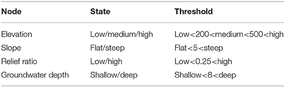
Table 1. Node states and thresholds.

Model Evaluation and Verification

Model sensitivity to findings relative to the HGM node was evaluated, and verification was undertaken by testing cases against two independent case files. In the first validation exercise, we used the case test file described above i.e., the digital data. For the second validation process, we collected field information on confirmed presence and HGM type of wetlands in the study area between March and May 2019. A total of 115 wetland point locations were recorded, and classified by HGM type according to Ollis et al. (2013). These data were attributed with values for the predictor nodes; these values were then converted to node states, and a second test case file developed i.e., a field data case test file. The independent case files were used to verify the training data set used to construct the Bayesian Network. Model performance was evaluated based on four standard outputs provided by Netica: node sensitivity; frequencies of predicted vs. actual HGM types; the number of times the model was “surprised” in predictions; and receiver operating characteristic (ROC) curves for each test case file, based on sensitivity and specificity (quality of test). The ROC graph provided a visual output for assessing model performance (Fawcett, 2006).

Results

In the Drakenstein study region, the dominant HGM type by area was “depression,” and “seep” by number; similarly, depression wetlands dominated by area and number for the CoCT area (Figure 2). There was little distinction between study region for unchannelled and channeled valley-bottom types (Figure 3; Table 2) confirming that both datasets could be combined in the terms of the modeling exercise.

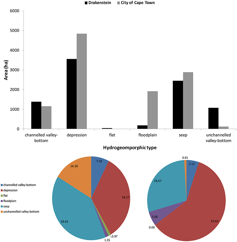
Figure 2. Total area (ha) of wetlands by HGM type (top) and proportion of wetlands by HGM type for the Drakenstein (bottom left) and CoCT (bottom right) regions.

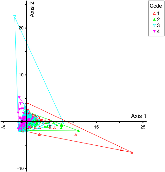
Figure 3. Principal Components Analysis for channeled valley-bottom (VB-C) and unchannelled valley-bottom (VB-U) wetlands based on area, perimeter, shape, and fractal dimension. Convex hull codes: 1, VB-C (Drakenstein); 2, VB-C (CoCT); 3, VB-U (Drakenstein); 4, VB-U (CoCT).

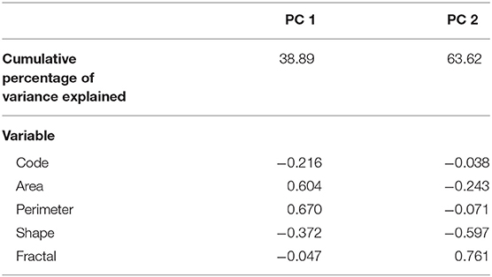
Table 2. Eigenvalues for the principal components analysis for channeled and unchannelled valley-bottom wetlands by municipality based on area, perimeter, shape, and fractal dimension.

A PCA indicated that morphometric variables were useful in distinguishing HGM types (Figure 4; Table 3). Here, variables describing polygon size (shape and area) accounted for the highest amount of variation in axis 1, while landscape characteristics (slope, stream order, and relief ratio) accounted for the highest amount of variation in axis 2. While elevation and groundwater depth did not come out strongly in the PCA, the box-and-whisker plots highlighted five morphometric variables (elevation, groundwater depth, relief ratio, slope, and shape) that provided clear distinctions between HGM group types (Figure 5). HGM types tended to be associated with upland vs. lowland zones to varying degrees (Figure 6). When median HGM type characteristics for morphometric variables that offered a degree of distinguishing power were plotted on a radar diagram, each HGM signature was unique (Figure 7).

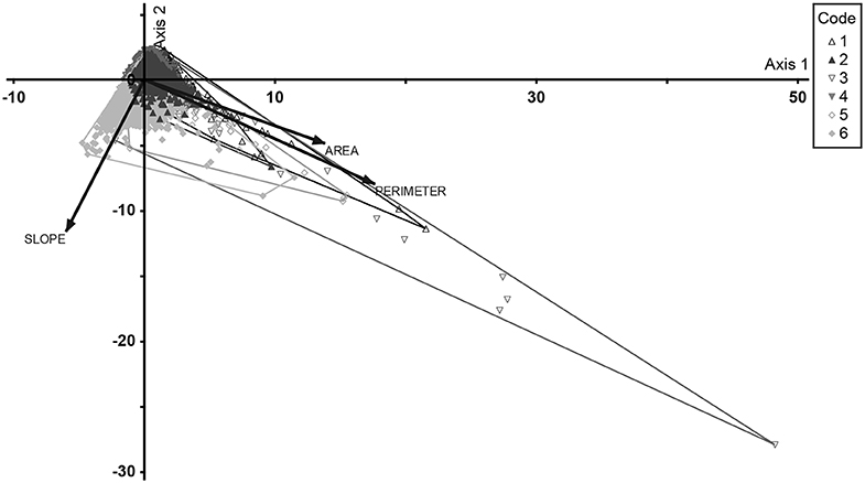
Figure 4. Principal Components Analysis biplot of wetland HGM types based on polygon morphometry; 1, channeled valley-bottom; 2, unchannelled valley-bottom; 3, depression; 4, flat; 5, floodplain; 6, seep. Vectors show variables with r² > 0.4.

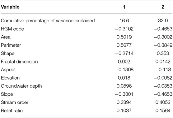
Table 3. Eigenvalues for the principal components analysis for wetland HGM types based on morphometric values of wetland polygons.

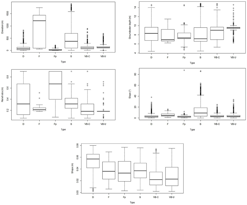
Figure 5. Box-and-whisker plots of HGM type by elevation (top left); groundwater depth (m below ground) (top right); relief ratio (center left); slope (center right); and shape (bottom), where D, depression; F, flat; Fp, floodplain; S, seep; VB-C, channeled valley-bottom; and VB-U, unchanelled valley-bottom. Boxes indicate median values of metrics per HGM type plus 25th/75th percentiles, while whiskers indicate data range.

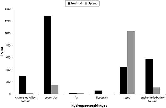
Figure 6. Count of wetlands by HGM type for the Drakenstein municipality for upland vs. lowland catchments.

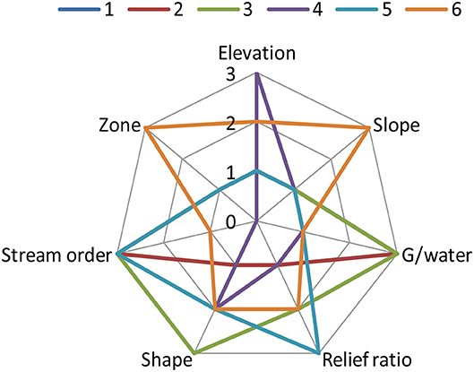
Figure 7. Radar plot of HGM signatures based on qualitative median scores of morphometric variables; 1, channeled valley-bottom; 2, unchannelled valley-bottom; 3, depression; 4, flat; 5, floodplain; 6, seep. Spokes reflect variables relating to each of six HGM types, qualitatively scored according to the categories in Table 1 in conjunction with their median values in Figure 5, where values 1–3 reflect categories as low/medium/high. Two additional variables (zone and stream order: Moolman, 2006) reflect HGM type majority membership for either upland or lowland zone (3, upland; 1, lowland) and Strahler stream order (1:500,000 scale).

The relationship between these variables and HGM type were linked by conditional probabilities in a Bn (Figure 8). By way of examples; at high elevations, there is a 71% probability that a wetland will be a seep, and this increases to an 87.4% probability when slope is steep. Conversely, for flat areas and low elevations, the most likely HGM type is depression at 54%. In our model, HGM type was most sensitive to elevation as a predictor variable (Table 4), with certain HGM types (seeps and flats) being more typically associated with higher elevations, while other HGM types (valley bottom and floodplains) are associated with lower elevations. Overall, prediction accuracy for the model had an error rate of 32.5% (Tables 5, 6). Notably, the HGM types with the poorest predictions were valley-bottom wetlands, which were incorrectly predicted as depressions or seeps. Conversely, prediction accuracies of seeps and depressions were high. The ROC plots further indicated that model predictions were generally good, but that the predictions were more accurate for the digital dataset than for the field-assessed HGM types (Figure 9).

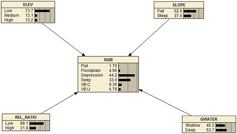
Figure 8. Bayesian network model for predicting wetland HGM type based on node states for elevation, slope, groundwater depth, and catchment relief ratio.

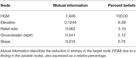
Table 4. Node sensitivity of variable nodes relative to the “HGM” node.

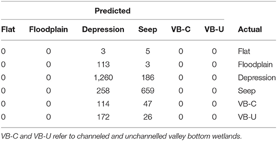
Table 5. Predicted vs. actual assignment of wetland HGM types based on test cases.

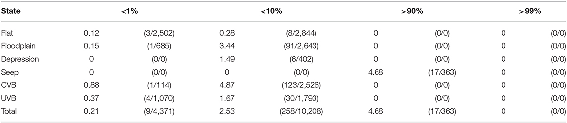
Table 6. Number of times the Bn was “surprised” for different probability values.

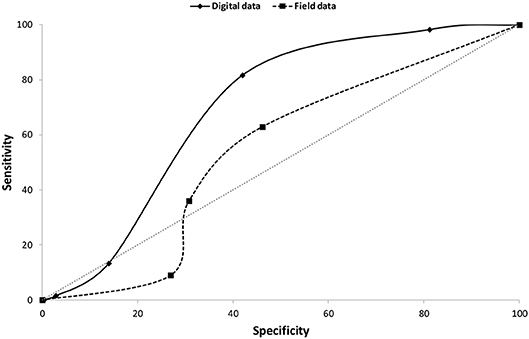
Figure 9. Receiver operating characteristic curves comparing the prediction accuracy of the digital data vs. the field data for HGM type in the study area.

Discussion

There is a growing demand for data on the ecological condition of wetlands, which is central to tracking improvements or deteriorations in the quality of this resource (Jacobs et al., 2010; Driver et al., 2011). This requires information not only on wetland location and extent, but also type. Since ecological condition varies on the basis of landscape context and HGM type (Jacobs et al., 2010; Gutzwiller and Flather, 2011), and wetland function varies by HGM type (Weller et al., 2007), management programmes cannot prioritize wetlands for conservation and rehabilitation without knowing HGM type. Information on total area per HGM type within a region is critical for national monitoring programmes, as well as for predicting loss rates over time. While comprehensive mapping of all three components (location, type, and ecological condition) is probably the most reliable approach, probability mapping provides statistical estimates of these parameters with a high level of repeatability at a fraction of the cost (Stein et al., 2016).

Probabilistic prediction of HGM type is an innovative approach. This is because it makes use of readily available spatial coverages to predict HGM type. Excellent 90 m digital elevation models are available globally, from which slope and relief ratio can be easily derived. Global datasets of groundwater depth are also available at the same resolution (for example, Fan et al., 2013). Our approach has the advantage in that it circumvents the need to use a landform image (i.e., natural features in the landscape: valleys, hills, etc.), which has previously been a problem because of limited availability and cost of sufficiently fine-scaled digital elevation models, such as those based on light detection and ranging (LIDAR) data.

In general terms, our model is a useful generic approach for improving the reliability of prediction for all major HGM types with the exception of valley-bottom wetlands. The poor performance in predicting valley-bottom wetlands may be simply a result of poor learning from the case files, given the relatively low prevalence of valley-bottom types in the chosen study area. It may be the consequence of not including a size metric in the model, since valley-bottom wetlands would typically be larger than depressions. Alternatively, there are encouraging results from other studies to specifically map valley-bottom wetlands (Collins, 2017), such that a HGM typing process could be successfully achieved by using a mix of ancillary data. This would involve an initial process of identifying all valley-bottom wetlands, followed by classifying the remaining wetlands using our model.

We recommend further research and model refinement/verification that improve the quality and resolution of input layers, and secondly in terms of translating the predictions of the Bn model to raster images of probabilities for each HGM type. For the former, consensus from the wetland scientific community on a suitable national elevation map, and an appropriate resolution (20 m: Hiestermann and Rivers-Moore, 2015; Melly et al., 2016; 30 m (USGS 1-arc minute with large voids) and 90 m (USGS 3-arc minutes void filled) will be needed. The higher the resolution of the DEM, the higher the anticipated reliability of the predictions. This would in turn form the basis for refined derived images from this map, including slope and relief ratio. For the latter, classification of the raster classes for each predictor variable into states, and subsequent translation of the HGM type model to a spatial probability product will assist with assigning HGM types to identified and mapped wetlands. This could then act as a hypothesis layer for testing against ongoing ground-truthing wetland surveys.

Data Availability Statement

The datasets generated for this study are available on request to the corresponding author.

Author Contributions

Study conceived, model development, and data analyses undertaken by NR-M. DK helped with writing, structure of manuscript, and conceptual approach. NJ contributed to introduction and discussion. SM undertook field work and contributed field validation dataset.

Conflict of Interest

The authors declare that the research was conducted in the absence of any commercial or financial relationships that could be construed as a potential conflict of interest.

Acknowledgments

We thank the South African Water Research Commission (Project Grant K5/2546) and the South African National Biodiversity Institute for funding and support of this research.

References

Anderson, J. E. (1991). A conceptual framework for evaluating and quantifying naturalness. Conserv. Biol. 5, 347–352. doi: 10.1111/j.1523-1739.1991.tb00148.x
Brinson, M. M. (1993). A Hydrogeomorphic Classification for Wetlands. U.S. Army Corps of Engineers, Technical Report WRP-DE-4, Washington, DC.
City of Cape Town (2017). Wetlands of Cape Town – Aquatic Features of the Biodiversity Network. Available online at: https://web1.capetown.gov.za/web1/OpenDataPortal/DatasetDetail?DatasetName=Wetlands (accessed August 23, 2019).
Clark Labs (2009). Idrisi Taiga v. 16.02. Clark University, Worcester, MA. Available online at: http://www.clarklabs.org
Collins, N. (2017). Mapping Valley-Bottom Wetland Areas. Unpublished Report. Free State Department of Economic Development, Tourism and Environmental Affairs, Bloemfontein, South Africa.
Colvin, C., le Maitre, D., Saayman, I., and Hughes, S. (2007). An Introduction to Aquifer Dependent Ecosystems in South Africa. WRC Report No. TT301/07. Water Research Commission, Pretoria.
Davidson, N. C., Fluet-Chouinard, E., and Finlayson, C. M. (2018). Global extent and distribution of wetlands: trends and issues. Mar. Freshw. Res. 69, 620–627. doi: 10.1071/MF17019
Day, E., Snaddon, K., Ractliffe, S. G., Ollis, D. J., and Murray, I. (2009). Provision of a Wetland GIS Cover for the Drakenstein Municipal Area. Prepared for the Department of Environmental Affairs and Development Planning Provincial Government of the Western Cape, Cape Town.
Driver, A., Nel, J., Snaddon, K., Murray, K., Roux, D., Hill, L., et al. (2011). Implementation Manual for Freshwater Ecosystem Priority Areas. WRC Report Number 1801/1/11. Water Research Commission, Pretoria. Available online at: http://bgis.sanbi.org/nfepa/project.asp
Euliss, N. H., Brinson, M. M., Mushet, D. M., Smith, L. M., Conner, W. H., Burkett, V. R., et al. (2013). Ecosystem services: developing sustainable management paradigms based on Wetland functions and processes, in Wetland Techniques: Volume 3:Applications and Management, eds J. T. Anderson and C. A. Davis (Dordrecht: Springer), 181–227.
Fan, Y., Li, H., and Miguez-Macho, G. (2013). Global patterns of groundwater table depth. Science 339, 940–943. doi: 10.1126/science.1229881
Fawcett, T. (2006). An introduction to ROC analysis. Pattern Recognit. Lett. 27, 861–874. doi: 10.1016/j.patrec.2005.10.010
Frimpong, E. A., Sutton, T. M., Engel, B. A., and Simon, T. P. (2005). Spatial-scale effects on relative importance of physical habitat predictors of stream health. Environ. Manage. 36, 899–917. doi: 10.1007/s00267-004-0357-6
Gordon, N. D., McMahon, T. A., and Finlayson, B. J. (1992). Stream Hydrology: An Introduction for Ecologists. Chichester: Wiley.
Guidugli-Cook, M., Richter, S. C., Scott, B. J., and Brown, D. R. (2017). Field-based assessment of wetland condition, wetland extent, and the National Wetlands Inventory in Kentucky, USA. Wetl. Ecol. Manag. 25, 517–532. doi: 10.1007/s11273-017-9533-3
Gutzwiller, K. J., and Flather, C. H. (2011). Wetland features and landscape context predict the risk of wetland habitat loss. Ecol. Appl. 21, 968–982. doi: 10.1890/10-0202.1
Hiestermann, J., and Rivers-Moore, N. A. (2015). Predictive modeling of wetland occurrence of KwaZulu-Natal, South Africa. S. Afr. J. Sci. 111:10. doi: 10.17159/sajs.2015/20140179
Horton, R. E. (1932). Drainage basin characteristics. Trans. Am. Geophysci. Union 13, 350–361 doi: 10.1029/TR013i001p00350
Horton, R. E. (1945). Erosional development of streams and their drainage basins: Hydrophysical approach to quantitative morphology. Geol. Soc. Am. Bull. 56, 275–370. doi: 10.1130/0016-7606(1945)56[275:EDOSAT]2.0.CO;2
Jacobs, A. D., Kentula, M. E., and Herlihy, A. T. (2010). Developing an index of wetland condition from ecological data: an example using HGM functional variables from the Nanticoke watershed, USA. Ecol. Indic. 10, 703–712. doi: 10.1016/j.ecolind.2009.11.011
Kotze, D. C. (2011). The application of a framework for assessing ecological condition and sustainability of use to three wetlands in Malawi. Wetl. Ecol. Manag. 19, 507–520. doi: 10.1007/s11273-011-9232-4
Kotze, D. C., Ellery, W. N., MacFarlane, D. M., and Jewitt, G. P. W. (2012). A rapid assessment method for coupling anthropogenic stressors and wetland ecological condition. Ecol. Indic. 13, 284–293. doi: 10.1016/j.ecolind.2011.06.023
McCune, B., and Mefford, M. J. (2011). PC-ORD. Multivariate Analysis of Ecological Data. Version 6.16 MjM Software, Gleneden Beach, OR.
Melly, B. L., Schael, D. M., Rivers-Moore, N. A., and Gama, P. T. (2016). Mapping ephemeral wetlands: manual digitisation and logistic regression modelling in Nelson Mandela Bay Municipality, South Africa. J. Environ. Manage. 25, 313–330. doi: 10.1007/s11273-016-9518-7
Midgley, D. C., Pitman, W. V., and Middleton, B. J. (1994). Surface Water Resources of South Africa 1990, Volumes I to VI. Reports No. 298/1.1/94 to 298/6.1/94. Water Research Commission, Pretoria.
Moolman, J. (2006). Slope Classification of Southern African Rivers. Available online at: http://www.dwaf.gov.za/iwqs/gis_data/RHPdata.htm (accessed August 23, 2019).
Norsys Software Corp. (2010). Netica v. 4.16. Available online at: http://www.norsys.com
Ollis, D. J., Ewart-Smith, J. L., Day, J. A., Job, N. M., Macfarlane, D. M., Snaddon, C. D., et al. (2015). The development of a classification system for inland aquatic ecosystems in South Africa. Water SA 41, 727–745. doi: 10.4314/wsa.v41i5.16
Ollis, D. J., Snaddon, C. D., Job, N. M., and Mbona, N. (2013). Classification System for Wetlands and Other Aquatic Ecosystems in South Africa. User Manual: Inland Systems. SANBI Biodiversity Series 22. South African National Biodiversity Institute, Pretoria.
R Development Core Team (2009). R: A Language and Environment for Statistical Computing. Vienna: R Foundation for Statistical Computing. Avaliable online at: http://www.R-project.org
Rivers-Moore, N. A., and Cowden, C. (2012). Regional prediction of wetland degradation in South Africa. Wetl. Ecol. Manag. 20, 491–502. doi: 10.1007/s11273-012-9271-5
Schulze, R. E. (1997). South African Atlas of Agrohydrology and Climatology. Report TT82/96. Water Research Commission, Pretoria.
Schumn, S. A. (1956). Evolution of drainage systems and slopes in badlands, at Perth Amboy, New Jersey. Geol. Soc. Am. Bull. 67, 595–646. doi: 10.1130/0016-7606(1956)67[597:EODSAS]2.0.CO;2
Stein, E. D., Lackey, L. G., and Brown, J. (2016). How accurate are probability-based estimates of wetland extent? results from a California validation study. Wetl. Ecol. Manag. 24, 347–356. doi: 10.1007/s11273-015-9460-0
USGS (2018). SRTM Digital Elevation/SRTM Void Filled 3-Arc. Available online at: https://earthexplorer.usgs.gov/
van Deventer, H., Nel, J., Maherry, A., and Mbona, N. (2014). Using the landform tool to calculate landforms for hydrogeomorphic wetland classification at a country-wide scale. S. Afr. Geogr. J. 98, 138–153. doi: 10.1080/03736245.2014.977812
van Deventer, H., Nel, J. L., Mbona, N., Job, N., Ewart-Smith, J., Snaddon, K., et al. (2016). Desktop classification of inland wetlands for systematic conservation planning in data-scarce countries: mapping wetland ecosystem types, disturbance indices and threatened species associations at country-wide scale using GIS. Aqu. Conserv. Mar. Freshw. Ecosyst. 26, 57–75. doi: 10.1002/aqc.2605
van Deventer, H., Van Niekerk, L., Adams, J., Dinala, M. K., Gangat, R., Lamberth, S. J., et al. (2020). National Wetland Map 5 – An improved spatial extent and representation of inland aquatic and estuarine ecosystems in South Africa. Water SA 46, 66–79. doi: 10.17159/wsa/2020.v46.i1.7887
Keywords: Bayesian network, classification, South Africa, Western Cape, probability, principal components analysis
Citation: Rivers-Moore NA, Kotze DC, Job N and Mohanlal S (2020) Prediction of Wetland Hydrogeomorphic Type Using Morphometrics and Landscape Characteristics. Front. Environ. Sci. 8:58. doi: 10.3389/fenvs.2020.00058
Received: 30 August 2019; Accepted: 28 April 2020;
Published: 22 May 2020.
Edited by:
John Pascal Simaika, IHE Delft Institute for Water Education, NetherlandsReviewed by:
Nick Davidson, Charles Sturt University, AustraliaMatthew Bird, University of Johannesburg, South Africa
Copyright © 2020 Rivers-Moore, Kotze, Job and Mohanlal. This is an open-access article distributed under the terms of the Creative Commons Attribution License (CC BY). The use, distribution or reproduction in other forums is permitted, provided the original author(s) and the copyright owner(s) are credited and that the original publication in this journal is cited, in accordance with accepted academic practice. No use, distribution or reproduction is permitted which does not comply with these terms.
*Correspondence: Nick A. Rivers-Moore, blackfly1@vodamail.co.za