Shear Wave Measurements of a Gelatin’s Young’s Modulus

Introduction

Gelatin is commonly used in experiments as an analog for the Earth’s crust, typically when studying magmatic dike propagation (e.g., Fiske and Jackson, 1972; Takada, 1990; Menand and Tait, 2002; Taisne and Tait, 2009; Kavanagh et al., 2018; Urbani et al., 2018; Derrien and Taisne, 2019; Pansino and Taisne, 2019; Pansino et al., 2019; Sili et al., 2019) or modeling fault slip behaviors (Corbi et al., 2011; Rosenau et al., 2017). It has been shown to scale the upper crust when prepared with a concentration between 2.5 and 5.0 wt% and cured at 5°C (Di Giuseppe et al., 2009; Kavanagh et al., 2013; van Otterloo and Cruden, 2016). At concentrations greater than 3.0 wt%, it can be described by the Maxwell model, so that its elastic and viscous components are in series (van Otterloo and Cruden, 2016).

Gelatin has a viscous component that can become prominent under certain circumstance, not usually associated to analog experiments of liquid-filled cracks. For samples prepared with low concentrations (<2.5 wt%) or cured at high temperatures (>15°C), the resulting gelatin more readily deforms in a viscous way, so that if strain is applied for a prolonged period of time, the material is permanently deformed. The characteristic time over which viscous deformation occurs is quantified by the Maxwell relaxation time, which van Otterloo and Cruden (2016) measure to be on the order of 0.1–1 s. Qualitatively speaking, such estimates are extremely short, considering that the elastic behavior of gelatin can be observed over a time scale of seconds to tens of minutes. For example, in the context of magma transport experiments, Sumita and Ota (2011) identified characteristic intrusion shapes associated to different types of deformation: liquid-filled cracks are associated to elastic deformation, diapir-like structures to ductile deformation, and dike-diapir hybrids in the transitional regime. The degree to which the tail of the intrusion (dike or diapir) shuts, as the liquid passes through the medium, likewise depends on the dominant component of deformation, as well as on the liquid viscosity. In this way, gelatin can be prepared to model a variety of processes associated a wide range of time scales, depending on its strength, the applied strain rate and the duration of strain. In our experiments, the extremely short duration of the applied stress (<1 s) ensures that the medium has a dominantly elastic response.

Knowledge of the material properties is important for scaling analog experiments. For example, the Young’s modulus and shear modulus, which quantify the material’s elastic and shear strength respectively, describe the capacity of the solid medium to deform due to an applied stress (Weertman, 1980; Dahm, 2000; Menand and Tait, 2002; Roper and Lister, 2007). Gelatin’s Young’s modulus is many orders of magnitude lower than that of the Earth’s crust, which enables crack propagation analog investigations. The necessary stress to overcome the fracture toughness can be easily generated in the laboratory and results in structures that are small enough to be contained in an experiment, with a time scale that is only minutes long. The Young’s modulus is also related to the fracture toughness parameter, which quantifies a solid’s resistance to fracture and thereby can be used to scale a dike’s vertical length (Weertman, 1971; Menand and Tait, 2002) and its propagation velocity (Dahm, 2000; Roper and Lister, 2007). Together, the Young’s modulus and fracture toughness control a dike’s aspect ratio by respectively restricting the ability of the dike to open and to propagate. Gelatin has a Young’s modulus 7–8 orders of magnitude lower than the crust (10³ – 10⁴ Pa, compared to 7 × 10⁹ – 6 × 10¹⁰ Pa; Ide, 1936; Menand and Tait, 2002; Kavanagh et al., 2013; Odbert et al., 2014), but a fracture toughness only 4 orders of magnitude lower (∼10² Pa⋅m^1/2, compared to ∼10⁶ Pa⋅m^1/2; Meredith and Atkinson, 1985; Menand and Tait, 2002; Kavanagh et al., 2013). Dikes therefore tend to have a smaller aspect ratio (length/thickness) in gelatin than in the crust, since the ratio of elastic to fracture forces is comparatively smaller; elastic deformation in gelatin requires comparatively less force and dikes are comparatively thicker.

A gelatin’s Young’s modulus is not easy to accurately predict (i.e., estimate without measurement), since it is dependent on many factors related to its preparation, like gelatin concentration, cooling history and water quality. Measurements are therefore important to characterize its strength, preferably in situ and around the time of the experiment (Menand and Tait, 2002; Di Giuseppe et al., 2009; Kavanagh et al., 2013). One method to do so is via rotational tests, which evaluate the viscous and elastic properties of a gelatin sample by relating the torque to the strain and the strain rate of a small gelatin sample (Di Giuseppe et al., 2009; van Otterloo and Cruden, 2016). This is an accurate, but destructive test that cannot be performed in situ on an experiment. In order to make in situ measurements of the Young’s modulus, deflection tests are traditionally employed, in which a load of known mass and diameter is placed onto the surface and the downward deflection is measured (Menand and Tait, 2002; Kavanagh et al., 2013). This method is accurate when many repeat tests are performed, varying the mass and diameter of the load, ensuring that the diameter remains much smaller than the gelatin container (<10% of its size), so that effects due to the gelatin sticking to the container wall are minimized (Kavanagh et al., 2013). For experiments in which part of the gelatin is embedded and inaccessible (e.g., in a layered gelatin), a secondary sample of gelatin from the same batch can be kept apart to measure its strength. For experiments studying fluid-filled fracture propagation, it is also possible to estimate the strength of an underlying layer based on the behavior of the fracture, in that its geometry changes as it enters an overlying layer of different strength (Rivalta et al., 2005). Each measurement methodology has its benefits, however none can directly measure the strength of embedded gelatins in a time-effective way.

We will describe a technique to measure a gelatin’s Young’s modulus, by taking advantage of its photoelastic property. This causes deviatoric stresses (i.e., total stress minus hydrostatic stress) to become apparent using polarizing filters (Figure 1; Taisne et al., 2011; Kavanagh et al., 2018; Pansino and Taisne, 2019), which linearly polarize light to an incidence angle. If there is no stress within the gelatin, light passes through the system and the filters merely dim the magnitude of transmitted light. However, if there is a deviatoric stress field, the light’s velocity retards heterogeneously, depending on the wavelength and stress level (Ramesh, 2000). As a result, it is possible to see the deviatoric stress field in real time, which has the appearance of a repeating rainbow pattern when using polychromatic light (e.g., white light) as a source. Each color band represents a contour along which the deviatoric stress is constant. If the deviatoric stress is defined as half of the maximum principal stress minus the minimum, (σ₁ − σ₃)/2, then it also corresponds to the maximum shear stress (Means, 1976). Indeed, only shear stresses seem to be visible when we place a static load on the surface of a gelatin (Figure 1b). The area just beneath the load has the maximum compressive stress, yet appears dark, as shear stresses are at a minimum at that location.

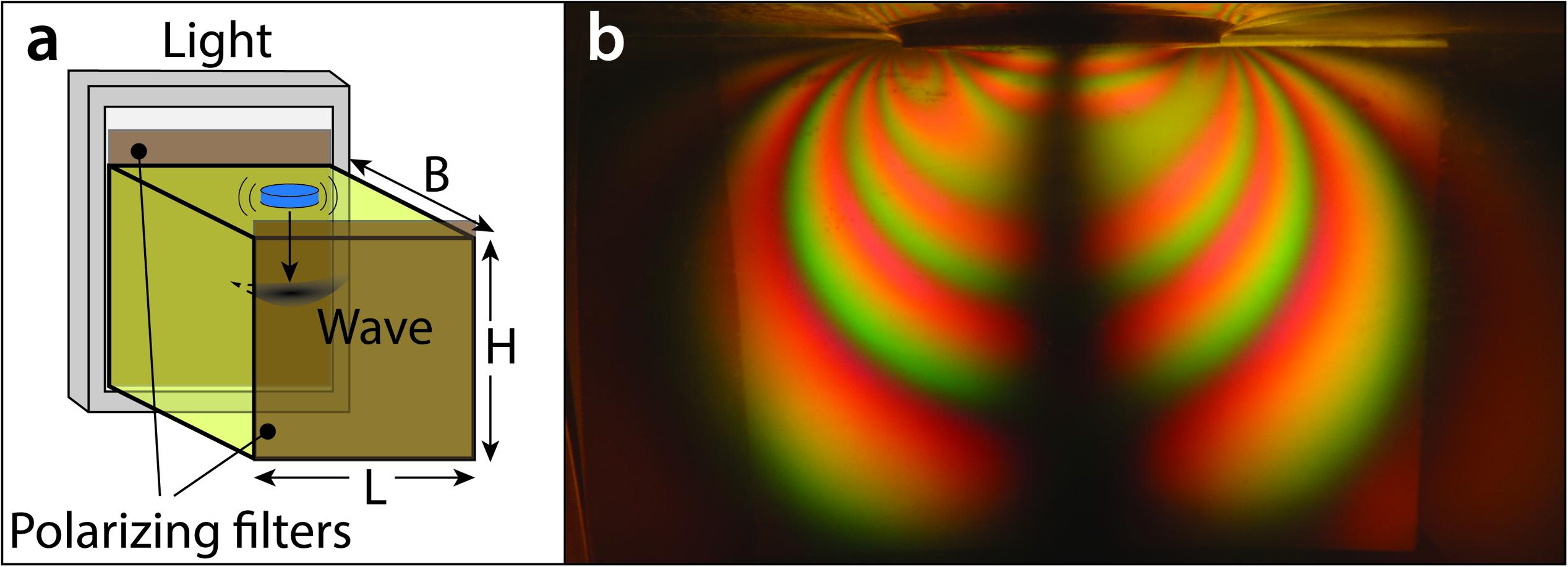
Figure 1. (a) Experimental setup. We arrange a block of gelatin with a set polarizing filters, one in front and one behind the block of gelatin. Light passes through the setup and the deviatoric stresses become apparent. We used tanks of different shapes and dimensions, indicated below in the methodology section. A small plastic disk (blue object) is placed on the surface and struck to generate shear waves from the same location each time. (b) The photoelastic behavior of gelatin. In this example, a surface load generates a deviatoric stress field, which appears as a repeating rainbow pattern. The spacing of these rainbow fringes indicates the stress gradient. This particular visualization of the stress field is for illustration only, and does not correspond to an experiment analyzed in this paper.

Shear waves, which are stress perturbations, similarly become visible using polarizing filters (Pansino and Taisne, 2019). The shear wave velocity, v_s, is related to the shear modulus, G, via

in which ρ is the solid’s density (Mavko, 2009). Since gelatin is very soft, shear waves are slow (∼m/s) and their propagation is visible to the naked eye or basic camera (Figure 2). By comparison, the pressure wave velocity, v_p, is faster and is related to the longitudinal modulus, M, by a similar equation (Parker and Povey, 2012):

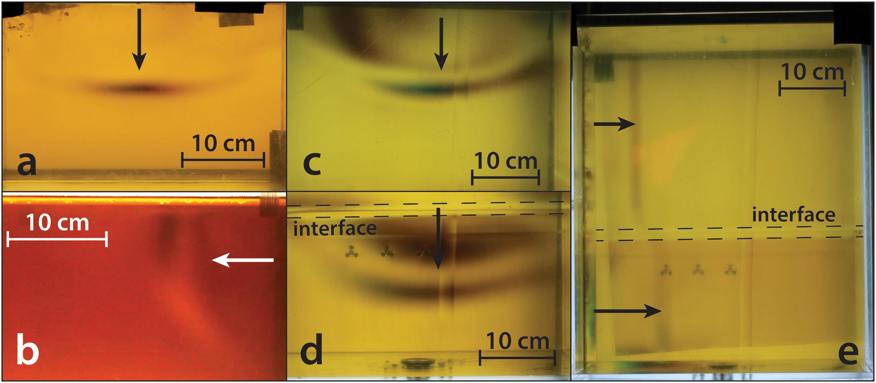
Figure 2. Waves are generated in different directions by strike a small block, placed on the surface, perpendicular to that direction. All images are side views of the experiments. (a,b) Representing vertical and horizontal propagation in a homogenous block (respectively, experiments Ex7 and Ex8 in Table 1). (c,d) Vertical propagation in two different layers (experiments L3a and L3b). The welded interface zone is indicated by the black dashed lines. (e) A broad, horizontally propagating wave in the same gelatin as (c,d). The wave separates due to the strength contrast between the layers. The welded zone shows a smooth velocity transition between the layers.

TABLE 1

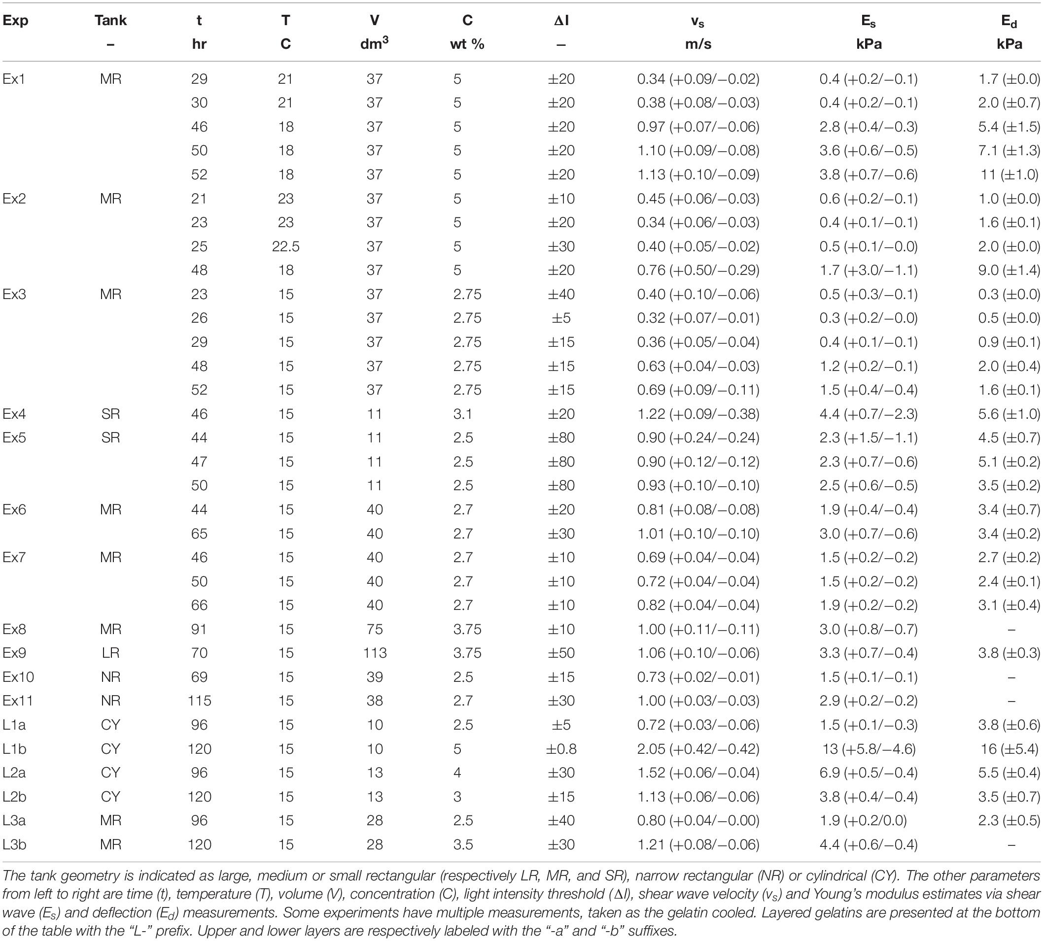
Table 1. Experimental conditions and results.

The G and M can be used to estimate the Poisson’s ratio, ν, of the material (Mavko, 2009),

Gelatin is usually assumed to be incompressible, so that ν = 0.5 (Menand and Tait, 2002; Rivalta et al., 2005; Kavanagh et al., 2013; Pansino and Taisne, 2019), however van Otterloo and Cruden (2016) show that it is a bit compressible, so that ν = 0.45. The Young’s modulus, E, is related to these parameters by,

(Mavko, 2009). The Poisson’s ratio has important implications for the ratio of the pressure wave velocity to shear wave velocity, such that pressure waves can be orders of magnitude faster in a material that has a Poisson’s ratio approaching 0.5. By comparison, crustal rocks have a Poisson’s ratio of 0.25, indicating that they are more compressible (Rubin, 1995; Taisne et al., 2011; Kavanagh et al., 2013). The compressibility of crustal rock causes the shape of the stress distribution due to a load to be different than in gelatin.

In this article, we describe in detail the technique introduced by Pansino and Taisne (2019) on how to use shear waves to measure a gelatin’s Young’s modulus in situ. This involves generating shear waves in a gelatin medium, which are captured in a video recording, and processing the videos to extract the wave velocity. Whereas, Pansino and Taisne (2019) briefly describe the methodology of using shear waves to measure the Young’s modulus, here we will go into more details, describing the experimental procedure, processing techniques that minimize the uncertainty on the results, validation against another measurement method and finally discuss the strengths and limitations of the technique.

Methods

Our basic procedure was to prepare a gelatin, repeatedly tap its surface to generate shear waves (Figure 1a), take a video recording of the waves, and finally processing the video to extract velocity measurements. We test the method on a collection of gelatin samples of varying volumes and concentrations, which were made in tanks of different H × B × L dimensions: 40 × 40 × 30 cm³ (rectangular), 50 × 50 × 50 cm³ (rectangular), and 33 × 19 × 22 cm³ (rectangular). These different tanks allowed us to explore the effect of volume and aspect ratio on shear wave measurements.

We also prepared additional subsets of gelatin for focused experiments. One subset was prepared to examine layered gelatins of varying strength contrasts, in order to assess the potential of the technique to measure the strength of both the overlying, directly accessible layer and the underlying, inaccessible layer. The strength contrasts allowed us to see the response of a wave traveling from a weak layer into a strong layer and vice versa. For these layered experiments, we used two different tank geometries, of dimensions 40 × 30 × 50 cm³ (rectangular) and 10² ×π× 100 cm³ (cylindrical), again to assess the method in tanks of different aspect ratios. Finally, for focused experiments examining wall effects, we prepared gelatins in a narrow, rectangular tank of dimensions 25 × 25 × 80 cm³.

Gelatin Preparation

To prepare each gelatin, we used animal derived Xiamen Yasin brand gelatin (250 bloom, 8–15 mesh) of concentrations between 2.5 and 5.0 wt%. To maximize the clarity of the gelatin, we dissolved the gelatin granules in deionized water with a splash of bleach, to inhibit bacterial growth. We slowly heated the mixture to 60°C while continuously stirring with a motorized, overhead stirrer. When the mixture had finished heating, we placed it in the tank and covered it with a film of oil to prevent evaporation and allowed it to solidify in a cold room at 15°C, the minimum temperature the room can achieve. Note that van Otterloo and Cruden (2016) found that, for long enough time scales, gelatins warmer than 15°C have a non-negligible viscous component, however in our experience, experimental dikes produced in our gelatins do not display any clear sign of plastic deformation (i.e., the gelatin returns to its initial position after the experiment concludes). Furthermore, the time scale associated to the shear wave experiments we describe is very short, so we assume they are dominated by elastic deformation. For layered gelatins, we repeated the process the subsequent day for a different concentration of gelatin and placed it on top of the original gelatin. We poured the fresh, hot liquid gelatin onto the solidified gelatin, which remelted a bit and created a cohesive contact between the two. Prior to pouring the new layer, we removed the oil layer and any oil residue floated to the top when the contact interface remelted. We also poured slowly to avoid the melting much of the lower layer. This produced an ∼2 cm thick, welded transitional region between the layers (marked in Figure 2), which matched the “strong interface” type described by Urbani et al. (2018) and Sili et al. (2019), for studies of sill emplacement. We did not make an experiment of a “weak interface,” such that the interface is sharp and the layers are disconnected, because we expected the wave would not effectively transfer from one layer to the next.

Wave Measurement Technique

We generated shear waves by placing a light, plastic cylindrical (5 cm diameter, 1 cm tall) pedestal on the gelatin surface and repeatedly tapping it perpendicularly to the intended propagation direction, producing sets of 40–50 waves, which radiate away in all directions (Figures 2a–d; Supplementary Videos 1–6). For some experiments, we placed the block on the center of the upper surface to focus on vertical, downward propagation (Figures 2a,c,d), while for other experiments, we placed it at the edge to focus on horizontal movement (Figure 2b). Gelatin is isotropic, so the direction of the wave propagation does not affect its velocity and it takes on a rounded appearance. For some of the layered gelatins, we substituted the block with an embedded, rigid plastic sheet, which we positioned along the wall of the tank. We struck this wall downward to produce a broad, horizontally propagating wave, which clearly demonstrates the velocity difference between the layers (Figure 2e). We recorded each set of waves with a DSLR camera, with 1280 × 800 pixels spatial resolution and 50 Hz temporal resolution.

We processed the videos in Matlab (vers. R2014b, R2019a; Mathworks, 2014, 2019) by tracking the change of light intensity, in the green channel, I, between successive frames, ΔI, in which regions of high change generally correspond to the position of the wave. For a video frame, a, ΔI is simply:

across an interval of b frames. To maximize the number of measurements from a wave, we use an interval of one or two frames; we generally use two to mitigate noisy results. To aid in the processing speed and measurement accuracy, we cropped the image to record the wave propagation along its clearest path. This usually took the form of a narrow vertical or horizontal strip of the video, originating from the location of the wave source and ending at the far wall of the tank (Figure 3a). We used a simple smoothing filter, finding the average value inside a moving cross, to remove any high-frequency variations and make the wave more-distinct from the background noise. This filter has the form of:

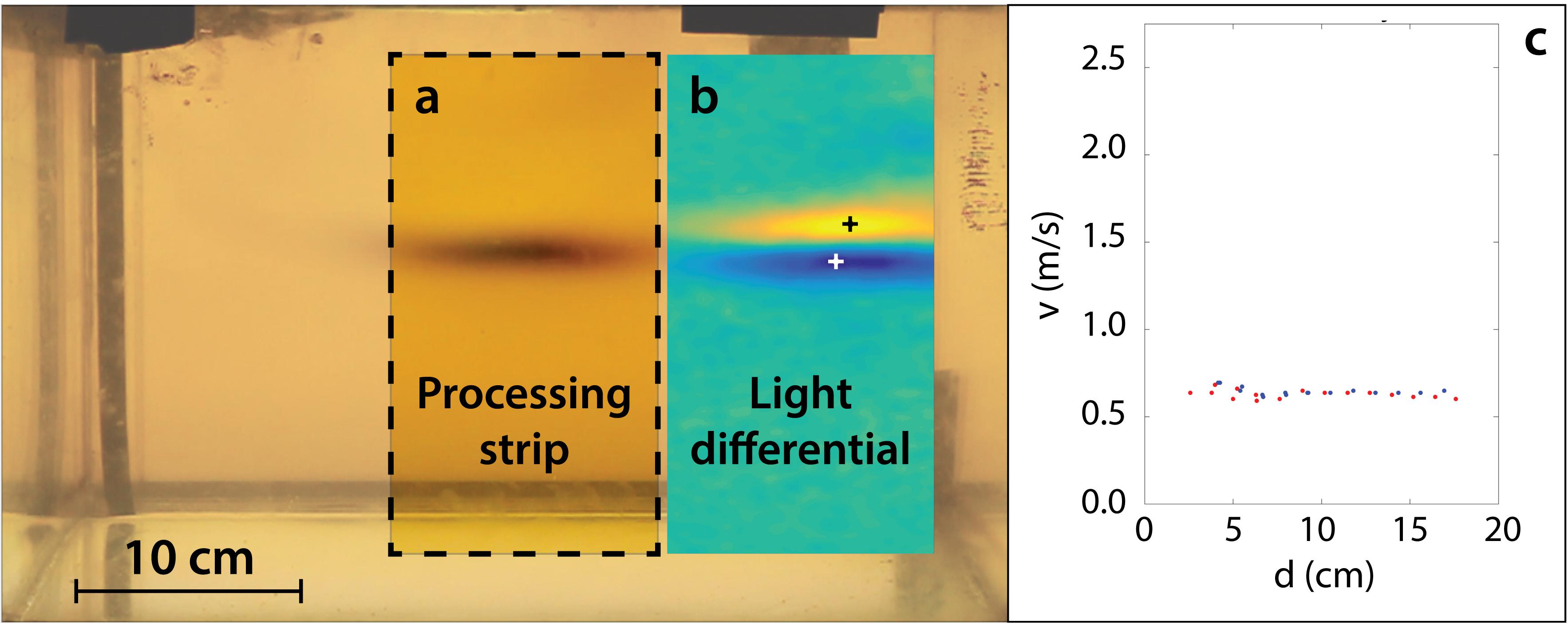
Figure 3. A processing example of experiment Ex7. (a) Frames are cropped to a narrow strip, aligned to the direction of the wave travel. (b) The difference in light intensity, ΔI, allows the wave to be identified. The yellow and blue regions respectively represent the wave’s previous and current location and the waves centers are marked by the “+” symbols. (c) The corresponding velocity is plotted against the travel distance along the processing strip. Red and blue dots correspond to the movement of the yellow and blue regions, respectively.

so that ΔI_s is the smoothed form of ΔI. From this point on, we will refer to ΔI_s as ΔI, for writing simplicity.

We track the wave position in ΔI (Figure 3b) by picking the centers of the regions with the highest and lowest magnitudes, which respectively indicate the waves previous and current locations. The velocity is estimated via the vertical travel distance (or horizontal, for such propagating waves) and the camera frame rate (Figure 3c). Without a size calibration, the velocity is given in pixel/s, however, by measuring an object in the video of known size (e.g., including a ruler in the video or using the tank apparatus as a size scale, measuring along the tank center), the velocity can be converted to SI units. Since a pair of frames generates a single measurement and each wave is captured over a handful of frame-pairs, each group of waves potentially generates hundreds of measurements, depending on how clearly they can be distinguished from the background noise.

Quality Control

To improve the quality of the results, we use criteria to accept or reject velocity measurements. The consistency of these measurements is a function of the magnitude of ΔI, in which measurements with large magnitudes (both positive and negative) tends to produce less-scattered results (Figure 4a). By setting a threshold and omitting smaller magnitudes, we can strongly improve the final velocity estimate (Figures 4b,c).

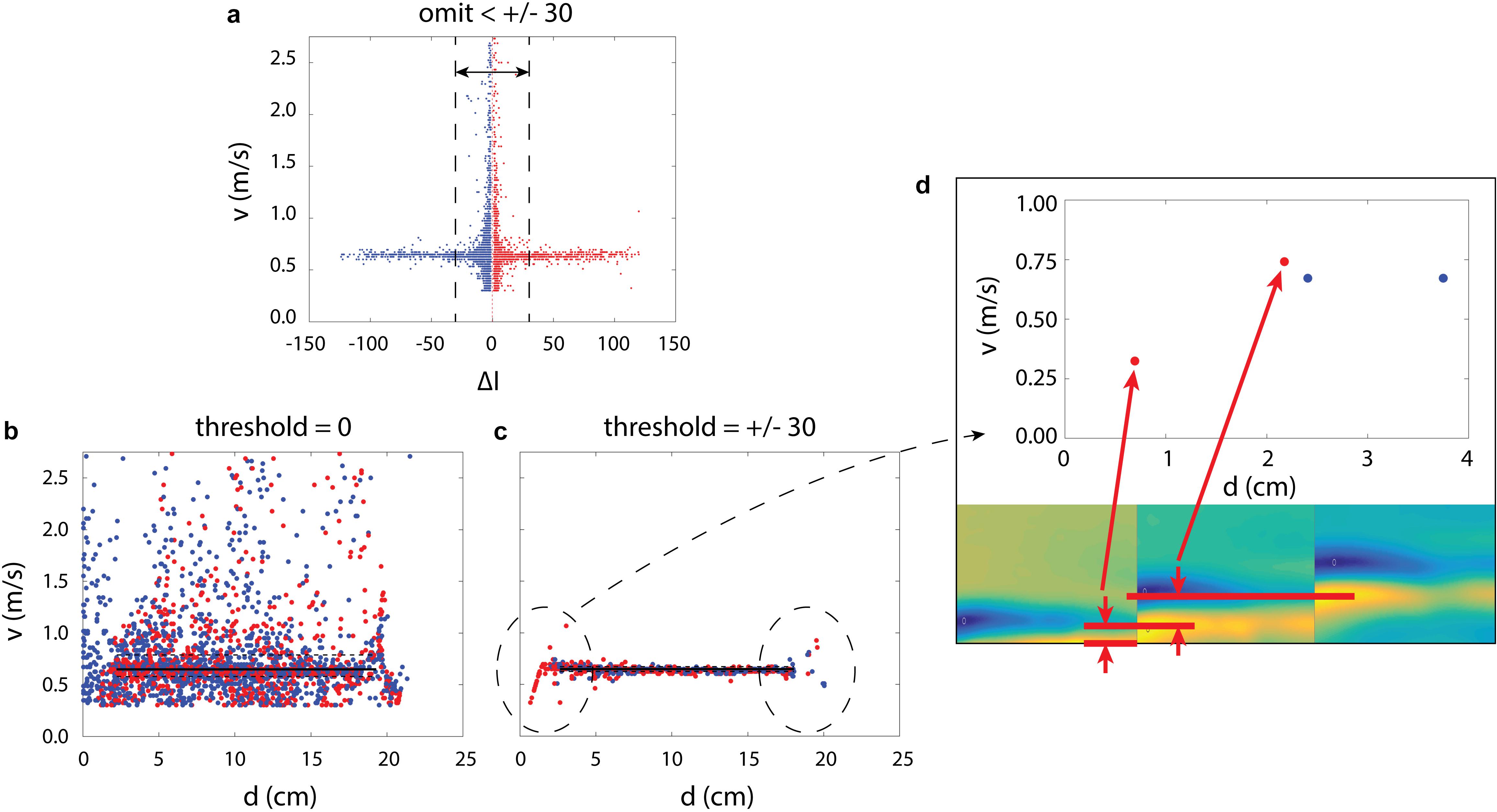
Figure 4. (a) Velocity measurements shown against the difference in light magnitude, ΔI, for experiment Ex7. Blue and red dots respectively represent negative and positive values. The measurements are more consistent at large magnitudes (both positive and negative). (b) With no threshold set, the velocity measurements are scattered. (c) Measurements within the magnitude of ±30, shown by the vertical dashed lines in subplot (a), are thrown out. Boundary artifacts remain in the measurements and are circled. (d) The artifacts appear when a wave enters or leaves the field of view. The red dots here correspond to the velocity of the yellow region and its velocity entering the frame is underestimated.

We also note that this technique produces artifacts in the measurements as a function of position, in which a wave entering or leaving the camera frame produces unreliable velocity results (Figure 4c). This is because a wave that has not fully entered view can still be detected, even though its center is not yet visible (Figure 4d). As the wave becomes fully visible in subsequent frames, the technique misjudges the distance the wave has travelled. We therefore omit measurements taken near the boundary of the video field of view.

Estimating the Young’s Modulus

We statistically estimate the Young’s modulus via the wave velocity distribution. We first estimate the median velocity and quantify the uncertainty using the median absolute deviation. We then estimate the shear modulus, for the median, lower and upper deviations of the wave velocity, via Equation (1) (G = ρv_s²), and the Young’s modulus, via Equation (4) [E = 2G (1 + ν)], where ν is assumed to be 0.45 (van Otterloo and Cruden, 2016). Note the density of gelatin is similar to water; for example, we measured the density of experiment Ex1 (Table 1), a 5.0 wt% gelatin, to be 1017 kg/m³. We have measured other gelatins, not in the study, to be between 1010 and 1030 kg/m³, depending on the concentration. We did not measure the density of each gelatin in this study, so for simplicity we assume all gelatins to have 1020 kg/m³.

Deflection Testing

For comparison with a different method, we also measure the Young’s modulus using a mass deflection test, following Menand and Tait (2002) and Kavanagh et al. (2013). A set of masses, m, were placed on a set of small pedestals of varying diameters, D, which in turn were placed on the gelatin surface. The gelatin deflects downward, in a relationship described by:

where w is the deflection and g is the acceleration of gravity. We performed these measurements directly on the upper free surface of each gelatin. For layered gelatins, in which the bottom layer is buried, we kept aside separate samples of the underlying layer for deflection testing. We estimated the Young’s modulus over 4–10 measurements via the mean and standard deviation of the measurements (taking more measurements in later experiments).

This technique produces its most-accurate results when the deflection is due to a load diameter that is small, relative to the size of the surface (Kavanagh et al., 2013). We note that, in practice, it is helpful for the deflection to be significant enough to be measured with little error; however, large deflections tend to leave the gelatin fractured and damaged, which may contaminate results.

Results

Shear Wave and Deflection Measurements

We compare the results of both the deflection and shear wave measurement methods (Table 1). For some experiments, we had not taken deflection measurements, so wave measurements are shown only to build a fuller dataset. This allows us to better view the strength measurements against various parameters like cooling time and gelatin concentration, both of which have a positive correlation (Figure 5).

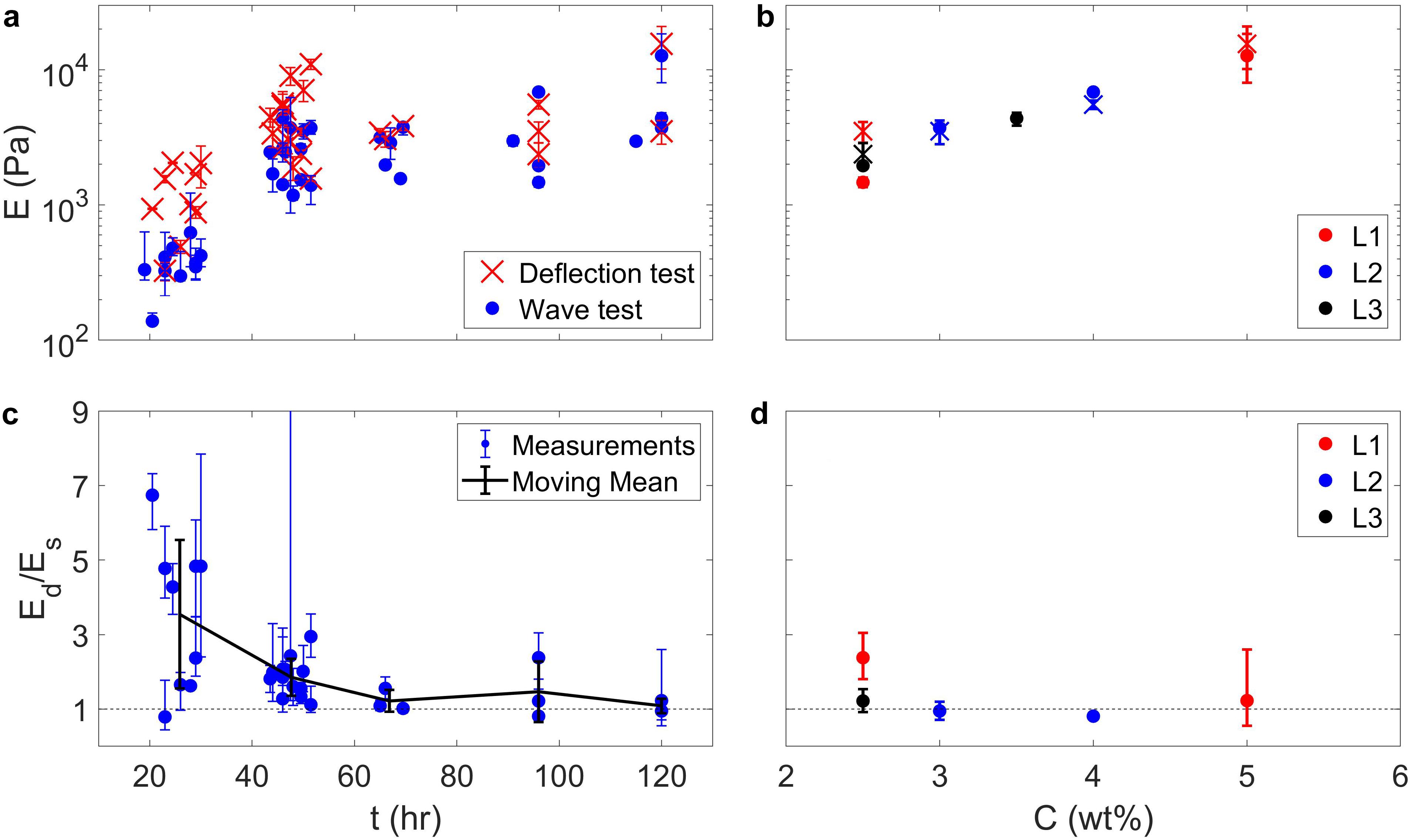
Figure 5. (a) Compiled Young’s modulus measurements, E, from both shear wave (blue ⋅) and deflection (red ×) measurements, shown against cooling time after placing the gelatin into a cold room refrigerator. (b) Measurements for only the layered gelatins, shown against concentration. Red, blue, and black colors respectively represent experiments L1, L2, and L3. The ⋅ and × symbols again represent shear wave and deflection measurements. (c,d) Similar plots, showing the ratio of measurements done by the deflection method to the shear wave method, so that a value of 1 represents a perfect match. Error bars on the individual data points represent the upper bound of one measurement divided by the lower bound of the other, and vice versa. The black line and error bars show the moving mean and standard deviation of these data points. The agreement improves for gelatins that have sufficient time to harden (>48 h). Note that adjacent plots share horizontal or vertical axes.

There is order-of-magnitude agreement between the two methods, which improves as gelatins harden (Figures 5a,c). For gelatins that are still cooling, the deflection method consistently produces higher estimates than the wave method, by a factor of up to 4.8, due to the core of the block being somewhat warmer and softer. This reveals that the waves quantify the strength of the interior region, whereas the deflection test quantifies the strength of the relatively hard surface. This is visible when viewing a propagating wave in such gelatins. We measured the wave velocity in experiment Ex3 along the upper surface of the gelatin and through the center of the block at 23 and 52 h. of cooling time (the first and last measurements described for Ex3 in Table 1). In the earlier recording, the wave propagated much faster horizontally than vertically, by a factor of 2 (Figure 6a), which corresponds to a factor of 4 in shear and Young’s moduli measurements (via Equation 1) and roughly explains the 4.8 factor between the wave and deflection techniques. By contrast, the gelatin had fully hardened in the later recording, so the vertical and horizontal velocity measurements match much more closely, within the measurement error bounds (Figure 6b).

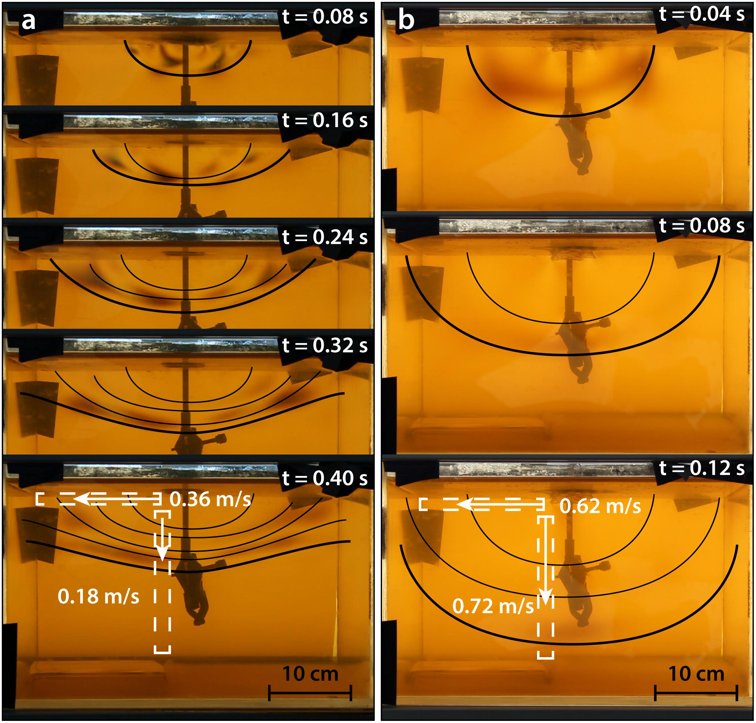
Figure 6. Two sequences of images from experiment Ex3, corresponding to the first and last measurement in Table 1. We highlight the approximate shape of the wave front with a bold line and previous positions with narrow lines. Velocity measurements were taken within windows defined by the white dashed boxes. All velocity measurements have an error of ∼10% of the measured value. (a) After ∼1 day of solidifying, the perimeter of the gelatin had hardened more than the middle. The wave propagates about twice as faster along the upper surface than through the center of the block. (b) The wave propagates at similar velocities along the upper surface and through the center. The measurements match within error bounds.

We also show the results of the layered gelatins (L1, L2, and L3 in Table 1). For experiments L1 and L2, we could not perform the deflection test directly on the gelatin’s upper surface due to the tank’s narrow size, since the gelatin cannot fully deflect and the resulting Young’s modulus is overestimated (Kavanagh et al., 2013). Instead, we measured the strength of separately stored samples, taken from the same batch of gelatin. Deflections tests for the lower layers were similarly done on separated samples taken from the same batch. There is good agreement between the two methods for all of the gelatins, including upper and lower layers (Figures 5b,d). Moreover, the uncertainty associated with shear wave measurements is generally smaller than deflection test, due to the high number of measurements that can be made using the technique.

Pressure Waves in Gelatin

Until now, we have discussed shear wave measurements assuming a 0.45 value for the Poisson’s ratio, following measurements by van Otterloo and Cruden (2016). However, we will explore the possibility to also measure pressure waves and thereby constrain the gelatin’s longitudinal modulus and Poisson’s ratio. While the polarizing filters enable clear shear wave visualization, pressure waves are not detectable in our experiment. This could be due to several factors including the wave velocity, which is too fast to detect. Indeed, Parker and Povey (2012) measured the pressure wave velocity to be between 1450 and 1500 m/s, for concentrations and temperatures associated to our experiments. In comparison with our shear wave measurements, v_s, on the order of 1 m/s, the pressure wave velocity, v_p, is three orders of magnitude faster. The relationship between the wave velocities to Poisson’s ratio, ν, can be shown by combining Equations (1–3):

and

The Poisson’s ratio is therefore expected to be extremely close to 0.5, the value that is commonly cited in published literature (Menand and Tait, 2002; Rivalta et al., 2005; Kavanagh et al., 2013; Urbani et al., 2018; Pansino and Taisne, 2019; Sili et al., 2019). Assuming that pressure waves are even visible using our polarizing filters, we would not be able to record them given our tank dimensions of <1 m and camera recording frequency of 50 Hz, which correspond to a maximum detectable velocity of 50 m/s.

In the example we presented in the introduction (Figure 1b), a static load exerts compressional and shear stresses on the underlying gelatin, but only the shear component is visible. We expect this is true for pressure waves as well, such that the compressional stress perturbation generates a secondary shear stress, which can be visualized. The shear strain, ε_s, due to the pressure wave is smaller than the compressive strain, ε_c, by a factor equal to the Poisson’s ratio, so that ε_s/ε_c = ν (Means, 1976). The shear modulus is similarly smaller than the Young’s modulus by a factor of G/E = 1/(2 + 2ν). For values of Poisson’s ratio discussed in this study, the shear stress, τ, associated to a pressure wave should be smaller than the compressive stresses, σ, by a factor of τ/σ = Gε_s/Eε_c ≈ 1/6, which means they are detectable with our visualization setup in terms of amplitude, assuming that the pressure wave amplitude is similar to that of the shear wave and that we have a high enough recording frequency.

Since the pressure wave velocity is likely too high to be visualized with our setup, we will instead investigate the extent of a static stress field, due to a dropped load, as a proxy for pressure wave velocity. When the load makes contact with a gelatin surface, it generates a pressure wave, a static stress field and a shear wave. The stress field propagates through the gelatin at the pressure wave velocity, after which the shear wave propagates. Although the stress field is due to compressional forces, the shear components are visible using the polarizing filters and we can visualize its extent with our relatively low recording frequency. We assume that the extent of the stress field, before the shear wave passes, sets a lower constraint on the pressure wave velocity.

To test this possibility, we prepared a small test gelatin (not shown in Table 1), with properties indicated in the caption of Figure 7, and dropped a small, 50 g mass onto the surface from a short, ∼1 cm height, to minimize the impact of the mass striking the gelatin and thereby mitigate jiggling. In the first moment after dropping the mass, a stress field was generated that extended several centimeters downward (Figures 7a,b), after which a shear wave propagated to the bottom of the vessel (Figure 7c). The visible extent of the initial stress field was ∼7 cm, so that at 50 Hz recording frequency, the maximum detectable velocity is 3.5 m/s (Figure 7d). Again, it is likely that the pressure wave was far faster than this, since it appeared in between camera frames, presumably at the velocity indicated by Parker and Povey (2012). We tracked the crest of the shear wave in Figure 7c and measured that the velocity was 0.85 m/s (Figure 7e), and via Equation (8) we estimate that the ν> 0.47 (matching the measurements by van Otterloo and Cruden, 2016). Even considering this lower, unrealistic estimate, we have 0.47 < ν < 0.5.

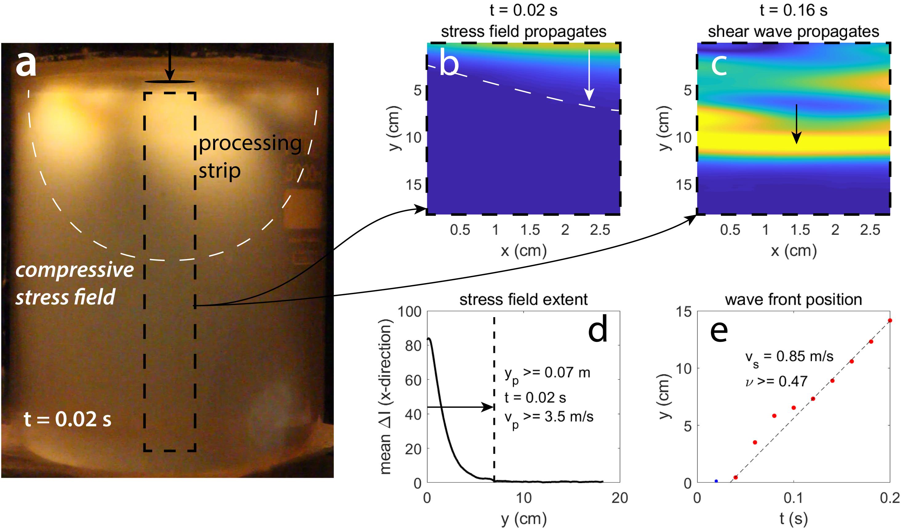
Figure 7. (a) A small gelatin not described in Table 1, 4 L in volume, 2.7 wt%, E = 2.1 kPa, cooled for 48 h. We dropped a 100 g, 2.5 cm diameter cylindrical mass onto the surface from a short height and recorded how the loading stress propagated. The processing strip illustrated by the black dashed box corresponds to the bounds of subfigures (b,c). (b) The ΔI of the stress field, in the first frame after dropping the mass. The white line shows the approximate extent of the stress field. (c) The ΔI of the stress field at t = 0.16 s (subtracting the frame for t = 0.14 s), showing the shear wave, which is indicated by the yellow region. (d) The mean ΔI values along the x-direction, showing the approximate extent of the stress field in the y-direction, which is marked by the vertical dashed line. The associated time interval and velocity are indicated. (e) The position of the shear wave front shown against time. The associated velocity is marked by the dashed line and labeled. The Poisson’s ratio is also labeled.

Discussion

Maximizing the Accuracy of the Technique

As we have shown, this technique can rapidly produce a large number of precise measurements. In section Quality Control we indicated that the quality of the results can be maximized by controlling which measurements are accepted, depending on the threshold light magnitude, ΔI, and by controlling the time interval over which measurements are performed. Increasing the threshold value and increasing the measurement interval both have the effect of increasing the precision at a cost of reducing the total number of results. However, depending on the wave velocity, the wave may only appear in a limited number of frames, so choosing a high interval can result in erroneous measurements.

The measured velocity generally shows lower scatter at large positive and negative values of ΔI (Figure 4a). The results that we presented in Table 1 indicate velocity measurements using a “good” ΔI threshold (also indicated in Table 1), which was manually selected and varies depending on the video (which in turn depends on the lighting conditions, the gelatin strength and the force used to generate waves). We processed the videos again for ΔI thresholds values of 1, 5, 10, 20, 40, and 80, using an interval of 1 frame (maximizing the capability to measure fast waves), to show that the results tend to improve at higher thresholds (Figures 8a,b). We use the median absolute deviation of the velocity measurements, normalized by the median velocity, to quantify the uncertainty (Figure 8b). At higher ΔI thresholds, poor measurements are omitted and the uncertainty decreases, so that the normalized deviation drops from 0.26 (±0.08) at a threshold of 1–0.08 (±0.05) at a threshold of 20. Note that some videos never meet high threshold values, so the number of data points diminishes toward the right end of the plots in Figures 8a,b. When using this technique, the best magnitude for the ΔI threshold needs to be assessed on a case-by-case basis, in order to obtain a maximum number of precise data.

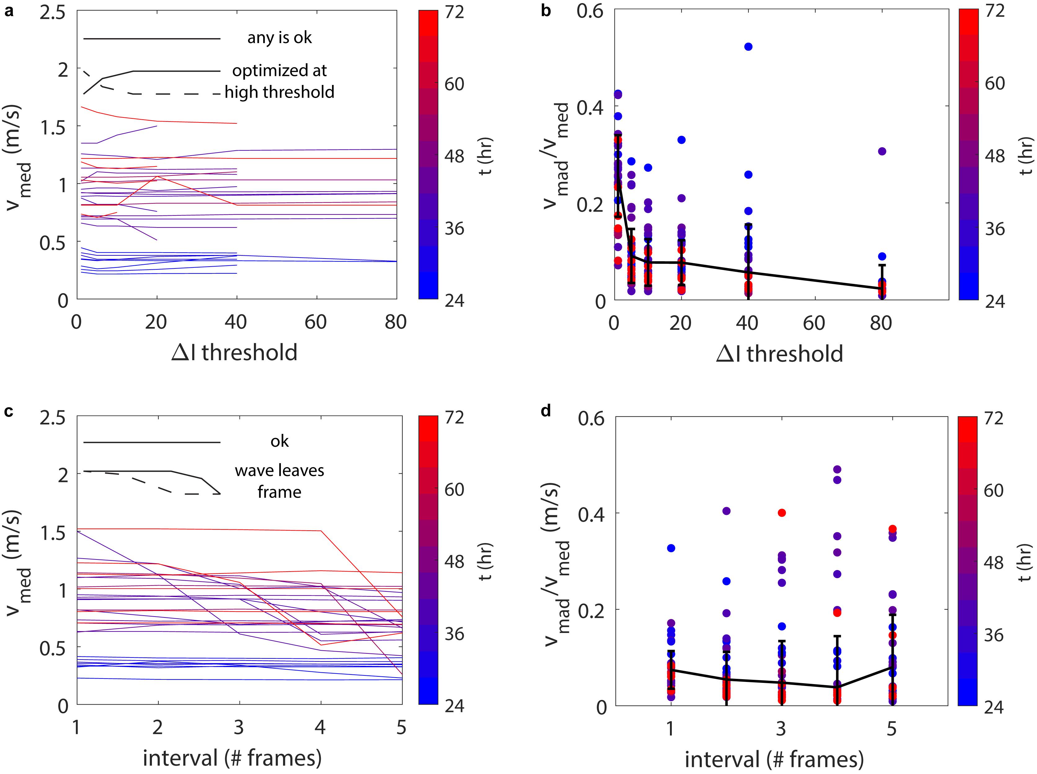
Figure 8. (a) The median velocity measurement of each experiment, v_med, shown against ΔI threshold. The color represents the cooling time in hours and each line represents a single experiment. (b) The median absolute deviation of these velocity measurements, v_mad, normalized by the median velocity. The black line and error bars respectively indicate the median values and the median absolute deviations of these data points for each ΔI threshold. (c) A similar plot to (a), against the measurement interval. (d) A similar plot to (b), against measurement interval. Subfigures (a,b) were done with an interval of 1 and (c,d) with ΔI thresholds indicated in Table 1.

We similarly analyze the effect of the measurement interval, using manually-selected “good” ΔI thresholds (Table 1) and intervals of 1, 2, 3, 4, and 5 frames (recorded at a frequency of 50 Hz). The velocity measurements generally show agreement, regardless of measurement interval, with the exception that some show a lower velocity at high intervals (Figure 8c). This is due to the wave entering, and then leaving, the camera frame during the interval, so that the measurement appears lower. In such cases, the crest of the wave is outside of view for part of the measurement, the nearest side of the wave is instead targeted, and the measurement is poor, appearing slower. In terms of uncertainty, the magnitude slightly decreases for larger intervals (Figure 8d), but as we just discussed, the median measurement can be poor if the wave both enters and leaves frames during the interval. The normalized deviation of the measurements changes from 0.07 (±0.04) at a 1 frame interval to 0.05 (±0.06) at 2 frames to 0.08 (±0.11) at 5 frames. In this sense, the measurements may be less reliable using long intervals, so we consider an interval of 2 frames (0.04 s) to be optimum.

Benefits and Limitations of the Technique

Our general assessment of the technique is that it is quick and simple to use and does not require a complex, nor expensive setup. It has the potential to make precise, repeatable measurements, with a low degree of uncertainty. The results can be trusted, as the velocity is, by definition, dependent on the medium strength.

Benefit: Time Efficiency

This technique is quick to perform. In terms of user time, only a few minutes are necessary to record a video of a sequence of shear waves, to upload it into the computer and adjust the inputs of the Matlab script (such as cropping the video). The processing time depends on the filtering, the extent to which the video is cropped and the total number of frames. For our setup, using a typical mid-range computer, a simple cross filter and a video cropped to ∼200 × 700 px, this corresponded to a few minutes of processing per minute of recorded video (50 Hz).

Benefit: in situ, Non-destructive Measurements

As shown in the results, this technique can be used to estimate the Young’s modulus of multiple gelatins, including those that are embedded and cannot be physically accessed. We note here that when a wave arrives at the interface between gelatin layers, some of its energy is transmitted to the next layer while some is reflected (the behavior that enables seismic reflection imaging; Fehler and Huang, 2002). When a wave arrives to a relatively weak layer, it appears to transmit a distinct wave that can then be measured. However, when a wave arrives to a much harder layer, it does not appear to make a distinct wave. This is possibly due to the stress associated with the wave, which in a soft material is relatively small, so that when it transfers to a harder material, its amplitude drops. For example, using the equation for the seismic reflection coefficient, R, with velocities of the upper and lower layers, v_u and v_l respectively, R = (ρv_l − ρv_u)/(ρv_l + ρv_u) (Onajite, 2014), experiment L1 has R ≈ 0.5. The combined effect of a low amplitude wave moving relatively fast in a hard gelatin challenges the technique to produce good results. As shown in Figure 2e, this can be overcome by generating a wave that propagates parallel to the interface.

We also note that our layered gelatins were prepared to have a strong, welded interface between the layers, which we expect maximizes transfer of the wave from one layer to the next. We did not prepare layered gelatins with a weak, disconnected interface, which we expect would inhibit this transfer.

Benefit: Aspect Ratio

Measurements can be performed on gelatins that are small in the lateral direction, allowing narrow or thin gelatins to be measured. There are potential wall effects, which we will describe below, but they are confined to a narrow region near the walls, so thinner gelatins can be measured more readily than via the mass deflection method. This has the caveat that waves need to be detected over multiple frames, meaning the user has to consider their camera’s frame rate, the expected wave velocity and the length of the gelatin. If a wave is too fast to be captured by a handful of frames, the measurement may not be accurate.

Limitation: Number of Frames Recording a Wave

The shear wave technique is most-effective for waves that can be recorded over many frames, yielding many measurements. When recording video, it is best to prioritize a high frame-rate over a high spatial resolution. Waves are generally wide and easily seen with the naked eye; however they move quickly in hard gelatins. Using a low frame rate reduces the number of measurements that can be made. When using the technique in small containers (<∼20 cm in its longest direction), it can be challenging to make a quality measurement without a high frame rate (≥50 Hz).

Limitation: Background Noise

Striking the gelatin to produce a shear wave may also cause the bulk gelatin to jiggle, producing a very noisy stress field. This is especially true for very hard gelatins (4.5–5.0 wt%; E >∼10⁴ Pa), which have noisier stress fields and exhibit fast wave velocities, so that they are difficult to accurately measure. Conversely, soft gelatins (2.5–3.0 wt%; E ∼ 10³ Pa) tend to attenuate weak movements and therefore exhibit very distinct, slow-moving waves, with little background noise, yielding good quality measurements. For example, the photos shown in Figures 2, 3 are of soft gelatins, displaying clearly distinct waves.

Limitation: Wall Effects

We also note that wave velocity is affected by the tank walls to a small degree. When using the shear wave technique in a narrow rectangular tank (experiment Ex10), we detected a velocity gradient, in which the core of the gelatin displayed slower velocities than close to the wall. The gradient is small and therefore not obvious (Figure 9a). However, by subdividing the video into narrow, parallel strips and processing them independently (i.e., a strip at the tank wall, one slightly inward, and so on to the tank center), the gradient can be quantified (Figure 9b). We find that the velocities are higher near the wall by a factor of ∼1.8 and that this affects the gelatin within the nearest few centimeters to the wall. This is due to the gelatin sticking to the rigid wall, which restricts its ability to displace, in turn reducing the shear strain due to the wave and increasing the effective shear modulus. To show this, we performed a similar experiment (Ex11), in which we first separated the gelatin from the wall, using a long, flat ruler (Figure 9c). We analyzed the video in the same way as Ex10 and the resulting velocity measurements show no obvious sign of the wall effect (Figure 9d). Note that in the images shown in Figure 9c, separating the gelatin from the wall generated a weak, heterogeneous stress field, as the gelatin shifted a bit, however this did not significantly affect the ability of the technique to measure the shear wave velocity, nor did it affect the results. Although it is possible to avoid the wall effects by manually separating the gelatin from the rigid wall, we consider them a limitation to the technique, as it cannot always be easily accomplished without damaging the gelatin (depending on the gelatin strength).

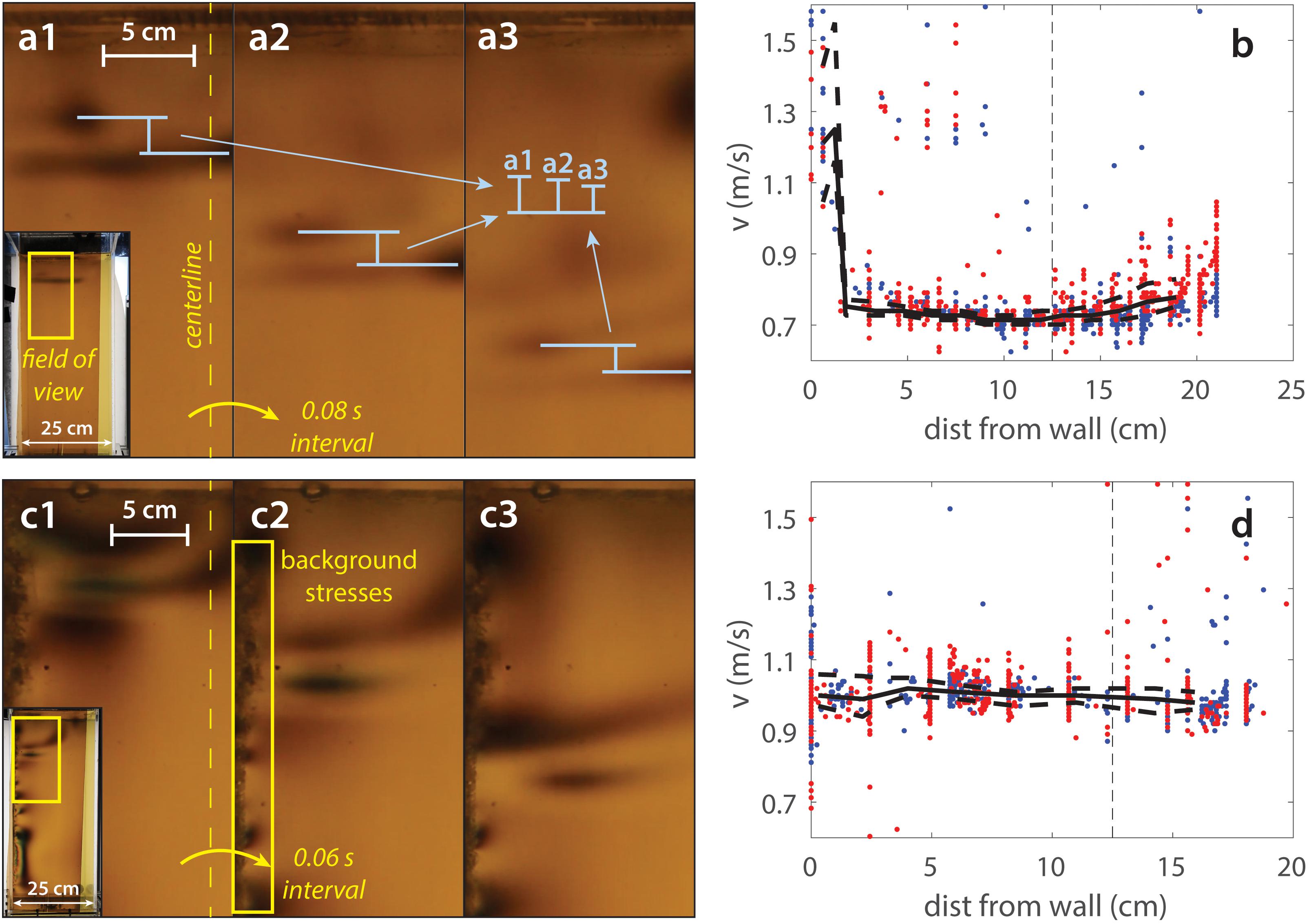
Figure 9. (a) A close-up view of a wave propagating downward (field of view indicated in inset), from Ex10. The wave travels slightly faster near the wall than in the center (yellow dashed line). The relative distance between offset wave crests decreases with time, indicating a higher velocity near the wall. (b) Velocity measurements at different distances from the wall. The wave appears faint near the wall, so measurements there are more scattered. The moving median values (horizontal solid line) and associated median absolute displacements (horizontal dashed lines) are shown, as well as the centerline (vertical dashed line). (c,d) Similar measurements from Ex11. We first separated the gelatin from the wall, causing small stress heterogeneities along the wall. The resulting velocity measurements show no obvious wall effect.

Conclusion

We present a method of measuring the Young’s modulus of gelatin, using shear wave velocity. Our technique has the potential to rapidly assess the Young’s modulus, with a high precision. We show that the measurements via this technique are comparable to the deflection method. The shear wave technique can make in situ, non-destructive measurements and can be used to measure gelatins in a variety of tank geometries and can even measure embedded gelatin layers, provided they are large enough or the camera recording speed is fast enough to track the wave through many frames. The technique is a simple, time-effective tool for researchers who use gelatin as an analog for the crust.

Author’s Note

This work comprises Earth Observatory of Singapore contribution no. 274.

Data Availability Statement

The datasets used for this study can be found in the Dataverse respository (https://doi.org/10.21979/N9/35QSJA).

Author Contributions

This work represents a method proposed by BT. SP and BT conceptualized the experimental design. SP performed and analyzed the experiments. The methodology behind the accompanying Matlab-based code was proposed by BT and SP wrote the code. The original manuscript was written by SP and edited by BT.

Conflict of Interest

The authors declare that the research was conducted in the absence of any commercial or financial relationships that could be construed as a potential conflict of interest.

Funding

This research was supported by the National Research Foundation Singapore (award NRF2015−NRF−ISF001−2437) and the Singapore Ministry of Education under the Research Centres of Excellence initiative.

Supplementary Material

The Supplementary Material for this article can be found online at: https://www.frontiersin.org/articles/10.3389/feart.2020.00171/full#supplementary-material

References

Corbi, F., Funiciello, F., Faccenna, C., Ranalli, G., and Heuret, A. (2011). Seismic variability of subduction thrust faults: insights from laboratory models. J. Geophys. Res. 116:B06304. doi: 10.1029/2010JB007993
Dahm, T. (2000). On the shape and velocity of fluid-filled fractures in the Earth. Geophys. J. Int. 142, 181–192. doi: 10.1046/j.1365-246x.2000.00148.x
Derrien, A., and Taisne, B. (2019). 360 intrusion in a miniature volcano: birth, growth, and evolution of an analog edifice. Front. Earth Sci. 7:19. doi: 10.3389/feart.2019.00019
Di Giuseppe, E., Funiciello, F., Corbi, F., Ranalli, G., and Mojoli, G. (2009). Gelatins as rock analogs: a systematic study of their rheological and physical properties. Tectonophysics 473, 391–403. doi: 10.1016/j.tecto.2009.03.012
Fehler, M. C., and Huang, L. (2002). Modern imaging using seismic reflection data. Ann. Rev. Earth Planet. Sci. 30, 259–284. doi: 10.1146/annurev.earth.30.091201.140909
Fiske, R. S., and Jackson, E. D. (1972). Orientation and growth of Hawaiian volcanic rifts: the effect of regional structure and gravitational stress. Proc. R. Soc. Lond. A 329, 299–326. doi: 10.1098/rspa.1972.0115
Ide, J. T. (1936). Comparison of statistically and dynamically determined Young’s modulus of rocks. Proc. Nat. Acad. Sci. U.S.A. 22, 81–92. doi: 10.1073/pnas.22.2.81
Kavanagh, J. L., Burns, A. J., Hazim, S. H., Wood, E. P., Martin, S. A., Hignett, S., et al. (2018). Challenging dyke ascent models using novel laboratory experiments: implications for reinterpreting evidence of magma ascent and volcanism. J. Volcanol. Geotherm. Res. 354, 87–101. doi: 10.1016/j.jvolgeores.2018.01.002
Kavanagh, J. L., Menand, T., and Daniels, K. A. (2013). Gelatine as a crustal analogue: determining elastic properties for modelling magmatic intrusions. Tectonophysics 582, 101–111. doi: 10.1016/j.tecto.2012.09.032
Mavko, G. (2009). The Rock Physics Handbook: Tools for Seismic Analysis of Porous Media, 2nd Edn. Leiden: Cambridge University Press.
Means, W. D (ed.) (1976). “Mohr circle for stress,” in Stress and Strain (New York, NY: Springer). doi: 10.1007/978-1-4613-9371-9_9
Menand, T., and Tait, S. (2002). The propagation of a buoyant liquid-filled fissure from a source under constant pressure: an experimental approach. J. Geophys. Res. 107:2306. doi: 10.1029/2001JB000589
Meredith, P. G., and Atkinson, B. K. (1985). Fracture toughness and subcritical crack growth during high-temperature tensile deformation of Westerly granite and Black gabbro. Phys. Earth Planet. Int. 39, 33–51. doi: 10.1016/0031-9201(85)90113-X
Odbert, H. M., Ryah, G. A., Mattioli, G. S., Hautmann, S., Gottsmann, J., Fournier, N., et al. (2014). “Volcano geodesy at the Soufrière hills volcano, montserrat: a review,” in The Eruption of Soufrière Hills Volcano, Montserrat from 2000 to 2010, Vol. 39, eds G. Wadge, R. E. A. Robertson, and B. Voight (London: The Geological Society Memoirs), 195–217. doi: 10.1144/M39.11
Onajite, E (ed.) (2014). “Chapter 2 – understanding seismic wave propagation,” in Seismic Data Analysis Techniques in Hydrocarbon Exploration (Amsterdam: Elsevier), 17–32. doi: 10.1016/B978-0-12-420023-4.00002-2
Pansino, S., Emadzadeh, E., and Taisne, B. (2019). Dike channelization and solidification: time scale controls on the geometry and placement of magma migration pathways. J. Geophys. Res. 124, 9580–9599. doi: 10.1029/2009JB018191
Pansino, S., and Taisne, B. (2019). How magma storage regions attract and repel propagating dikes. J. Geophys. Res. 124, 274–290. doi: 10.1029/2018JB016311
Parker, N. C., and Povey, M. J. W. (2012). Ultrasonic study of the gelation of gelatin: phase diagram, hysteresis and kinetics. Food Hydrocoll. 26, 99–107. doi: 10.1016/j.foodhyd.2011.04.016
Ramesh, K. (2000). Digital Photoelasticity – Advanced Techniques and Applications. Heidelberg: Springer-Verlag, doi: 10.1007/978-3-642-59723-7
Rivalta, E., Böttinger, M., and Dahm, T. (2005). Buoyancy-driven fracture ascent: experiments in layered gelatine. J. Volcanol. Geotherm. Res. 144, 273–285. doi: 10.1016/j.jvolgeores.2004.11.030
Roper, S. M., and Lister, J. R. (2007). Buoyancy-driven crack propagation: the limit of large fracture toughness. J. Fluid. Mech. 580, 359–380. doi: 10.1017/S0022112007005472
Rosenau, M., Corbi, F., and Dominguez, S. (2017). Analogue earthquakes and seismic cycles: experimental modelling across timescales. Solid Earth 8, 597–635. doi: 10.5194/se-8-597-2017
Rubin, A. M. (1995). Propagation of magma-filled cracks. Ann. Rev. Earth Planet. Sci. 23, 287–336. doi: 10.1146/annurev.ea.23.050195.001443
Sili, G., Urbani, S., and Acocella, V. (2019). What controls sill formation: an overview from analogue models. J. Geophys. Res. 124, 8205–8222. doi: 10.1029/2018JB017005
Sumita, I., and Ota, Y. (2011). Experiments on buoyancy-driven crack propagation around the brittle–ductile transition. Earth Planet Sci. Lett. 304, 337–346. doi: 10.1016/j.epsl.2011.01.032
Taisne, B., and Tait, S. (2009). Eruption versus intrusion? Arrest of propagation of constant volume, buoyant, liquid-filled cracks in an elastic, brittle host. J. Geophys. Res. 114:B06202. doi: 10.1029/2009JB006298
Taisne, B., Tait, S., and Jaupart, C. (2011). Conditions for the arrest of a vertical propagating dyke. Bull. Volcanol. 73, 191–204. doi: 10.1007/s00445-010-0440-1
Takada, A. (1990). Experimental study on propagation of liquid-filled crack in gelatin: shape and velocity in hydrostatic stress condition. J. Geophys. Res. 95, 8471–8481. doi: 10.1029/JB095iB06p08471
Urbani, S., Acocella, V., and Rivalta, E. (2018). What drives the lateral versus vertical propagation of dikes? Insights from analogue models. J. Geophys. Res. 123, 3680–3697. doi: 10.1029/2017JB015376
van Otterloo, J., and Cruden, A. R. (2016). Rheology of pig skin gelatine: defining the elastic domain and its thermal and mechanical properties for geological analogue experiment applications. Tectonophysics 683, 86–97. doi: 10.1016/j.tecto.2016.06.019
Weertman, J. (1971). Velocity at which liquid-filled cracks move in the Earth’s crust or in glaciers. J. Geophys. Res. 76, 8544–8553. doi: 10.1029/JB076i035p08544
Keywords: shear waves, analog experiments, gelatin, Young’s modulus, polarized light
Citation: Pansino S and Taisne B (2020) Shear Wave Measurements of a Gelatin’s Young’s Modulus. Front. Earth Sci. 8:171. doi: 10.3389/feart.2020.00171
Received: 04 February 2020; Accepted: 04 May 2020;
Published: 29 May 2020.
Edited by:
Yosuke Aoki, The University of Tokyo, JapanReviewed by:
Daniele Trippanera, King Abdullah University of Science and Technology, Saudi ArabiaEleonora Rivalta, GFZ Helmholtz Centre Potsdam, Germany
Copyright © 2020 Pansino and Taisne. This is an open-access article distributed under the terms of the Creative Commons Attribution License (CC BY). The use, distribution or reproduction in other forums is permitted, provided the original author(s) and the copyright owner(s) are credited and that the original publication in this journal is cited, in accordance with accepted academic practice. No use, distribution or reproduction is permitted which does not comply with these terms.
*Correspondence: Stephen Pansino, stepheng001@e.ntu.edu.sg