Development of Seismic Response Simulation Model for Building Structures with Semi-Active Control Devices Using Recurrent Neural Network


Division of Architecture, Sunmoon University, Asan-si 31460, Korea
Appl. Sci. 2020, 10(11), 3915; https://doi.org/10.3390/app10113915
Submission received: 7 May 2020
/
Revised: 29 May 2020
/
Accepted: 2 June 2020
/
Published: 5 June 2020
(This article belongs to the Special Issue Advances on Structural Engineering)
Abstract
:A structural analysis model to represent the dynamic behavior of building structure is required to develop a semi-active seismic response control system. Although the finite element method (FEM) is the most widely used method for seismic response analysis, when the FEM is applied to the dynamic analysis of building structures with nonlinear semi-active control devices, the computational effort required for the simulation for optimal design of the semi-active control system can be considerable. To solve this problem, this paper used recurrent neural network (RNN) to make a time history response simulation model for building structures with a semi-active control system. Example structures were selected of an 11-story building structure with a semi-active tuned mass damper (TMD), and a 27-story building having a semi-active mid-story isolation system. A magnetorheological damper was used as the semi-active control device. Five historical earthquakes and five artificial ground motions were used as ground excitations to train the RNN model. Two artificial ground motions and one historical earthquake, which were not used for training, were used to verify the developed the RNN model. Compared to the FEM model, the developed RNN model could effectively provide very accurate seismic responses, with significantly reduced computational cost.
1. Introduction
Much research on the development of seismic response reduction technologies has been conducted to date. Various types of active, semi-active, and passive control systems have provided good seismic response reduction. Although active control devices can best reduce seismic responses, practicing engineers have yet to fully embrace them, in large part because of the challenges of large power requirements, and concerns about their stability and robustness. Because of these defects of active control systems, research on semi-active control systems is being actively conducted [1,2,3]. Semi-active control devices have been applied to various types of control systems, such as the tuned mass damper [4,5], base or mid-story isolation system [6,7], outrigger damper system [8], coupled building control system [9], and bracing system with dampers [10]. Once the application plan of the semi-active control system for building structures subjected to earthquake loads is decided, a control algorithm is one of the most important factors to affect seismic response reduction performance. Therefore, a number of studies on semi-active control strategies have been carried out by researchers [11,12,13].
Many numerical simulations should be carried out to evaluate the control performance of the semi-active control algorithm. In particular, the soft computing-based control algorithms, such as fuzzy logic controller (FLC), genetic algorithm (GA), and artificial neural network (ANN), require many more time history analysis runs to find the global optimal solution [14,15]. Usually, a state–space model of the building structure is used to obtain the structure’s dynamic responses under various excitations, considering the semi-active control forces [16]. Thanks to this representative state–space model, simulation tests of semi-active control efficiency and robustness can be realized. The state–space model is built according to the finite element (FE) model, namely the mass, damping, and stiffness matrices, exclusively. The differential equations should be solved to obtain the dynamic responses of the building structure using a state–space model. If the number of degrees of freedom (DOF) of the EF model is large, or the time-step of the state–space analysis is small for stable solving of the differential equations, the computational time for simulation tests of the semi-active control system could be considerable. In this case, the solution search area of soft computing techniques including evolutionary algorithm may be narrowed to significantly reduce the optimization time, resulting in failure to find the global optimal solution. To solve this problem, the effective dynamic response simulation model of the building structure with a semi-active control system is developed using deep learning technique.
At present, almost every industry is affected by artificial intelligence (AI). Since an artificial neural network (ANN) has been applied to structural engineering, many studies on various topics have been conducted [17]. Recent rapid advances in deep learning have greatly expanded its application possibility to structural engineering, such as design optimization [18], structural system identification [19], structural assessment and monitoring [20], structural control [21], and finite element generation [22]. Among these topics, this study focused on structural system identification and structural control. Previous studies have successfully used ANN, fuzzy inference system, adaptive neuro fuzzy inference system, etc. to present the dynamic characteristics of the structural control device [23,24]. However, research on the dynamic response prediction of an entire building structure with semi-active control devices has rarely been performed to date.
Several types of neural networks (NNs) are used in various engineering research areas. Feed-forward neural network (FNN) is one of the simplest forms of ANNs. The application of FNNs is found in computer vision and speech recognition. Convolutional neural network (CNN) is a class of deep neural networks and most commonly applied to the analysis of visual imagery. Kohonen self-organizing NN is generally used to recognize patterns in the data. Its application can be found in medical analysis to cluster data into different categories. Recurrent neural network (RNN) works on the principle of saving the output of the layer and feeding this back to the input to help in remembering some information in the previous time-step [25,26]. Because of these characteristics, RNN is known as a type of NN well-suited to time series data such as stock prices. The RNN’s ability to model time series forecasting problems is adequate for the development of the dynamic response prediction model for the buildings with semi-active control devices. The application of any other kind of NNs to time series forecasting problems is rarely found. Among various deep learning techniques, RNN is used to make the time series response prediction model in this research.
This study selected a semi-active tuned mass damper (STMD) and a semi-active mid-story isolation system (SMIS) as semi-active control systems. A magnetorheological damper was used as the semi-active control device. The STMS was applied to the top story of an 11-story building structure, while the SMIS was used for a 27-story building structure. The displacement, acceleration, and inter-story drift of the selected stories were used for output data of the RNN model. Ground motion data, command voltage, and previous step output date were selected for input data. Python was used to program the RNN model generation codes, and Tensorflow was employed as a deep learning library. Ten ground excitations and another three excitations were used for training and verification of the RNN model, respectively. The numerical simulations showed that compared to the FE model, the developed RNN model was effective in providing very accurate seismic responses, with significantly reduced computational cost.
2. Use of the Recurrent Neural Network
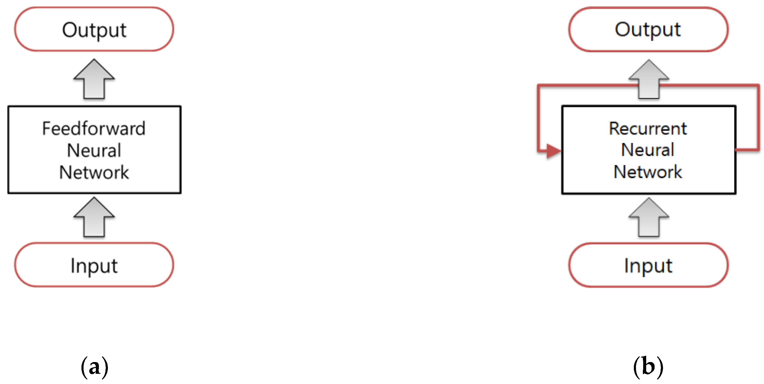
The FNNs tend to be straightforward networks that associate inputs with outputs. They allow signals to travel one way only from input to output, as shown in Figure 1a. FNN has no feedback (loops); i.e., the output of any layer does not affect the same layer. In contrast, recurrent neural networks can have signals traveling in both directions, by introducing loops in the network, as shown in Figure 1b. RNN has been shown to be able to represent any measurable sequence-by-sequence mapping. Thus, RNN is being used nowadays for all kinds of sequential tasks, such as time series prediction, sequence labeling, and sequence classification. The RNN’s ability to model time series forecasting problems is adequate to the development of the dynamic response prediction model of the buildings with semi-active control devices.
If FNN is used for the dynamic response simulation model of a structure subjected to earthquake loads, the output responses of FNN are always equal given the same inputs (excitation and control command data). However, RNN has a mechanism by which it “remembers” the previous inputs, and produces an output based on all of the inputs. This mechanism causes the outputs of RNN to be determined based not only on the instant input values, but also on the trends (e.g., increase, decrease) of inputs. Accordingly, RNN can output different responses even when given the same inputs, resulting in a more accurate dynamic response simulation model.
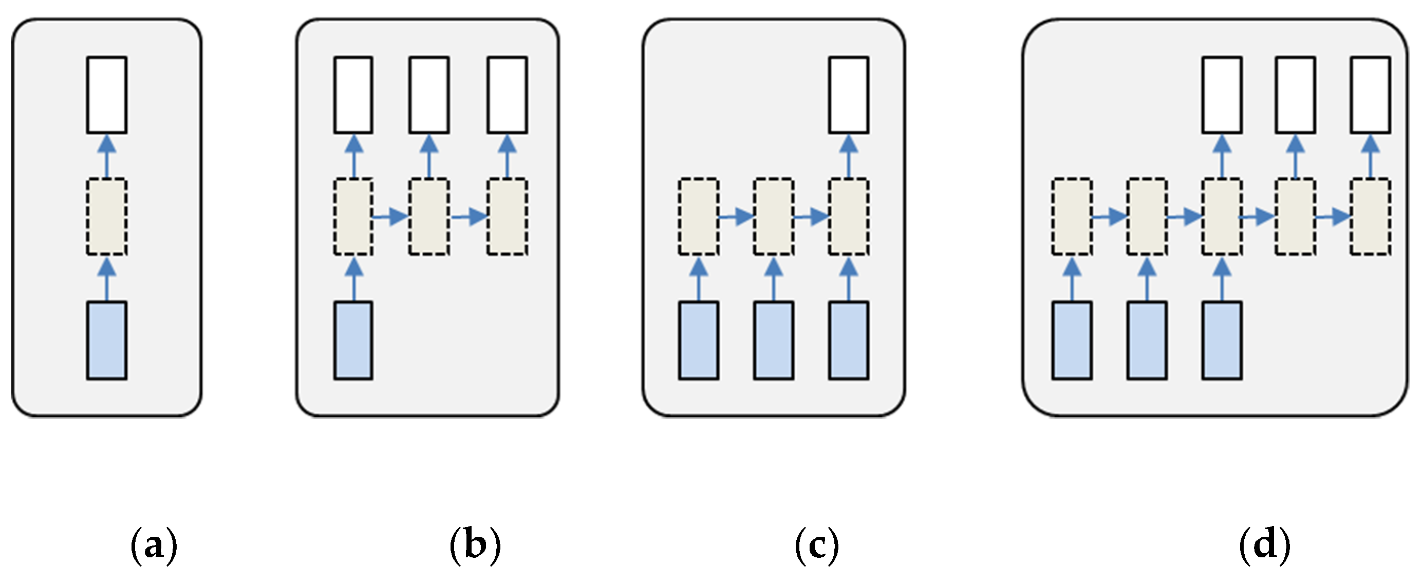
RNN can be structured in multiple ways, as shown in Figure 2. The bottom rectangle is the input, leading to the middle rectangle, which is the hidden layer, leading to the top rectangle, which is the output layer. The one-to-one model is the typical neural network with a hidden layer and does not consider sequential inputs and outputs. This model is frequently used for the image classification. The one-to-many model provides sequential outputs with one input, and thus it is generally applied to the image captioning that takes an image and outputs a sentence of words. The many-to-one model accepts sequential inputs and provides one output. The many-to-many model uses sequential inputs and sequential outputs. This model is suitable for machine translation. For example, an RNN reads a sentence in English and then outputs a sentence in French. Among the four architectures, the many-to-one model is the most suitable for the dynamic response simulation model. Several sequential ground motion and control command data are given as ‘many’ inputs, while the dynamic responses of the specific time-step are provided as ‘one’ output in this study. The input and output variables of the RNN model are described in detail in the following section.
A number of semi-active control devices have been used for the dynamic response reduction of building structures subjected to earthquake loads. One of the most promising semi-active control devices is the magnetorheological (MR) damper, because it offers many advantages, such as force capacity, high stability, robustness, and reliability. Because of their mechanical simplicity, high dynamic range, and low power requirements, MR dampers are considered to be good candidates for reducing structural vibrations, and they have been studied by a number of researchers for the seismic protection of civil structures [27,28,29]. A number of models for dynamic simulation of the MR damper have been proposed by many researchers [30,31,32]. These models can be classified into parametric and non-parametric models. The Bouc–Wen model is the most common parametric model. Most of the non-parametric models are based on soft computing techniques, such as neural networks, fuzzy logic, fuzzy neural network, neuro-fuzzy system, and deep neural networks [23,27,32].
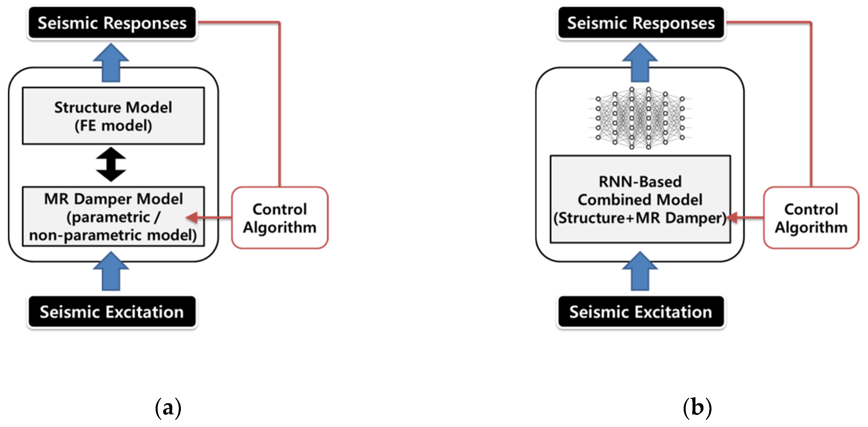
Figure 3a shows a schematic of the conventional simulation model using a parametric or non-parametric model of the MR damper and FE model of a structure. Because parametric or non-parametric models for presenting the nonlinear behavior of an MR damper are not available in conventional finite element analysis software, the control force of the MR damper is considered by using external mathematical programming language, such as Matlab. Bathaei et al.’s study [33] created the structural model of the building in OpenSees, while applying the Bouc–Wen model in Matlab. The connection between the two programs was made through TCP/IP. Otherwise, the simplified FE model and MR damper model are considered together in state–space analysis using a mathematical programming tool. In any case, the FE model of a structure and the nonlinear model of MR damper are separately considered. This comes at the cost of high computing time and complicated simulation process. This fact can render the design process inefficient. In order to defeat this shortcoming, this paper proposes the integrated simulation model considering nonlinear interaction between a structure and semi-active control devices simultaneously using RNN, as shown in Figure 3b.
3. Example Building Structures with Semi-Active Control System
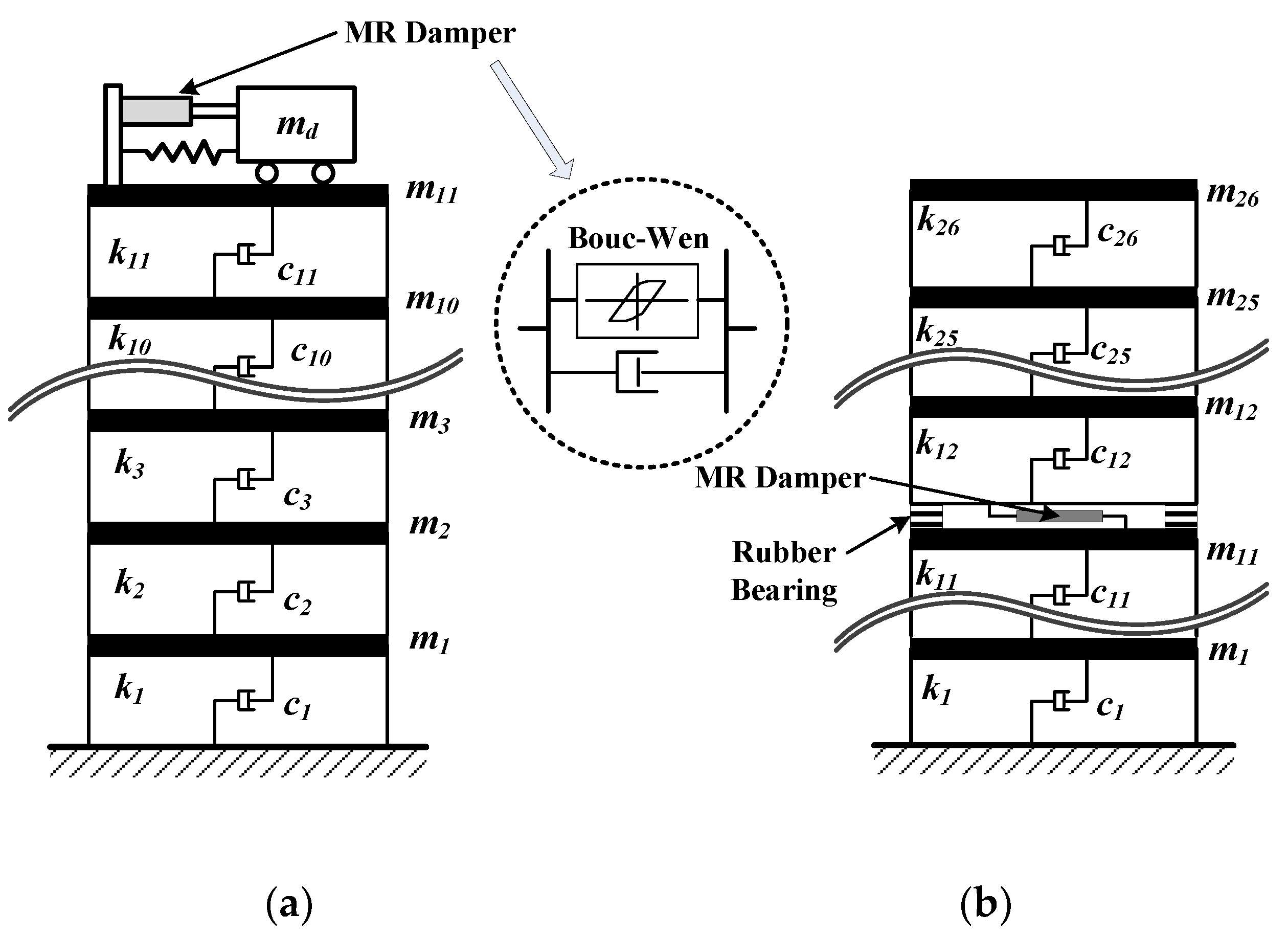
Two structural models with semi-active control systems shown in Figure 4 were used in this study. Figure 4a shows the first model (Example 1), which was an 11-story building with STMD installed on the top story; meanwhile, Figure 4b shows the second model (Example 2), which was a 26-story building with SMIS installed between the 11th and 12th stories. In the two example structures, the MR damper was used as a semi-active control device. The Bouc-Wen model, which is the most commonly used parametric model, was used to present the nonlinear behavior of the MR damper. Table 1 lists the structural properties of the two example buildings, which were obtained from previous studies [33,34].
The horizontal stiffness of each story shown in the table was modeled by the equivalent shear spring. Table 1 shows the mass of each story, which has one DOF without torsion. Structural damping of both models according to Rayleigh assumptions was considered to be 2%. A mass ratio of 2% for STMD was used for vibration control in Example 1. The first mode natural period of Example 1 was equal to 0.89 s. The period of STMD was tuned to that of Example 1. The structural properties of Example 2 were obtained from Shiodome Sumitomo building in Tokyo, Japan [34], which has a mid-story isolation system that is composed of multi-rubber bearing, lead damper, and steel damper. Two hysteresis-type dampers, i.e., lead and steel dampers, were replaced by MR dampers in Example 2.
The Bouc–Wen model parameters for MR dampers were selected from the experiment conducted at Washington State University [35], and these parameters were scaled to have the appropriate maximum MR damper force for each model. A parameter study was performed by changing the maximum capacity of the MR damper force, and the values of 500 and 2750 kN were selected for Examples 1 and 2, respectively. Ten MR dampers were used for the optimal seismic control of Example 2. The voltage sent to the MR damper varied within the range 0–10 V.
4. Training and Verification Data for the RNN Model
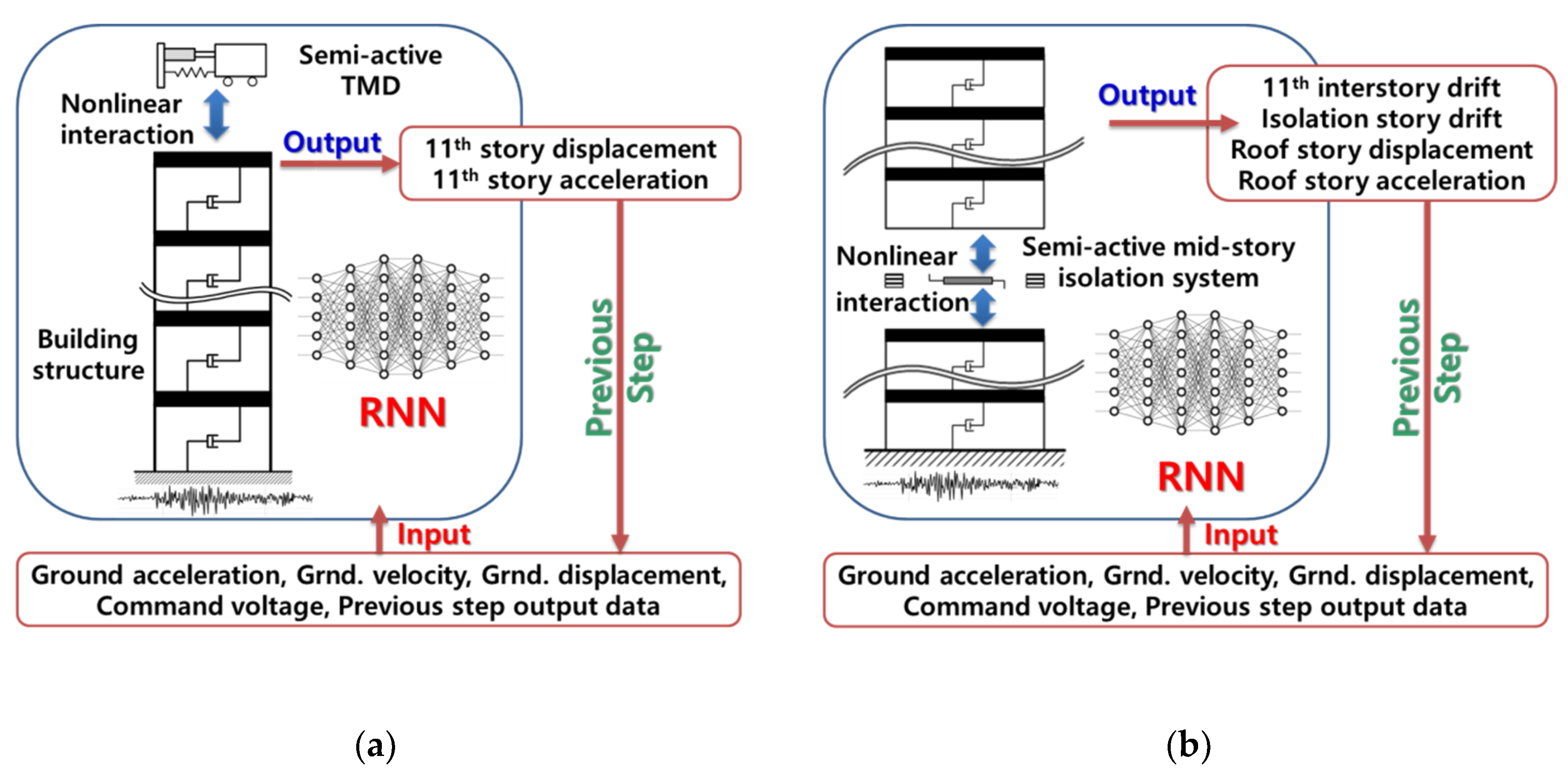
The data required for the development of the RNN model were divided into training and verification data. Training data were used to learn and adjust the weights and biases of neural networks. Verification data were applied to the trained RNN model to substantiate whether or not the model was suitable when unknown input data were applied, and the seismic responses of the structure were to be predicted. Appropriate training and verification datasets should be prepared to develop accurate RNN simulation models for building structures having semi-active control systems. Figure 5 shows that the RNN model presents seismic responses by considering nonlinear interaction between the semi-active control devices and structures as an integrated simulation model. The acceleration, velocity, and displacement of ground motion, and command voltage sent for the MR damper were selected as inputs of the RNN model for both Examples 1 and 2 structures. Because the outputs of the previous time-step could be good reason for the outputs for the next time-step, they were also included in the inputs. In Example 1, the roof story displacement and acceleration were selected as outputs of the RNN model to evaluate the safety and serviceability of the structure, respectively. The RNN model of Example 2 provided four outputs of the 11th inter-story drift, isolation story drift, and the roof story displacement and acceleration. Because the peak inter-story drift of Example 2 occurred at the 11th story that was just below the isolator installed story, it needed to be included in the outputs, and was evaluated to validate the safety requirements. If the damping force of the MR damper is selected as the outputs of the RNN model as required, the control output can be easily provided by the RNN model.
Table 2 shows a list of the seismic excitations used for the training and verification processes of the RNN model. The 10 ground excitations for training consisted of five historical earthquakes, and five artificial ground motions. Two artificial ground motions and one historical earthquake that were not used for training were applied to verification of the trained RNN model. Two types of ground motions, i.e., far-field and near-field, and different levels of P.G.A. were considered to increase the adaptability of the RNN model to diverse ground motions. The ground accelerations of the 13 seismic excitations listed in Table 2 were numerically integrated to generate ground velocity and displacement time histories for inputs of the RNN model.
The ground acceleration is usually modeled as a filtered Gaussian process. The most common model is a Kanai–Tajimi shaping filter that is a viscoelastic Kelvin–Voigt unit (a spring in parallel with a dashpot), carrying a mass that is excited by a white noise [36]. The Kanai–Tajimi shaping filter [37] presented in Equation (1) was used to generate the seven artificial earthquakes in Table 2:
where, rad/s, .
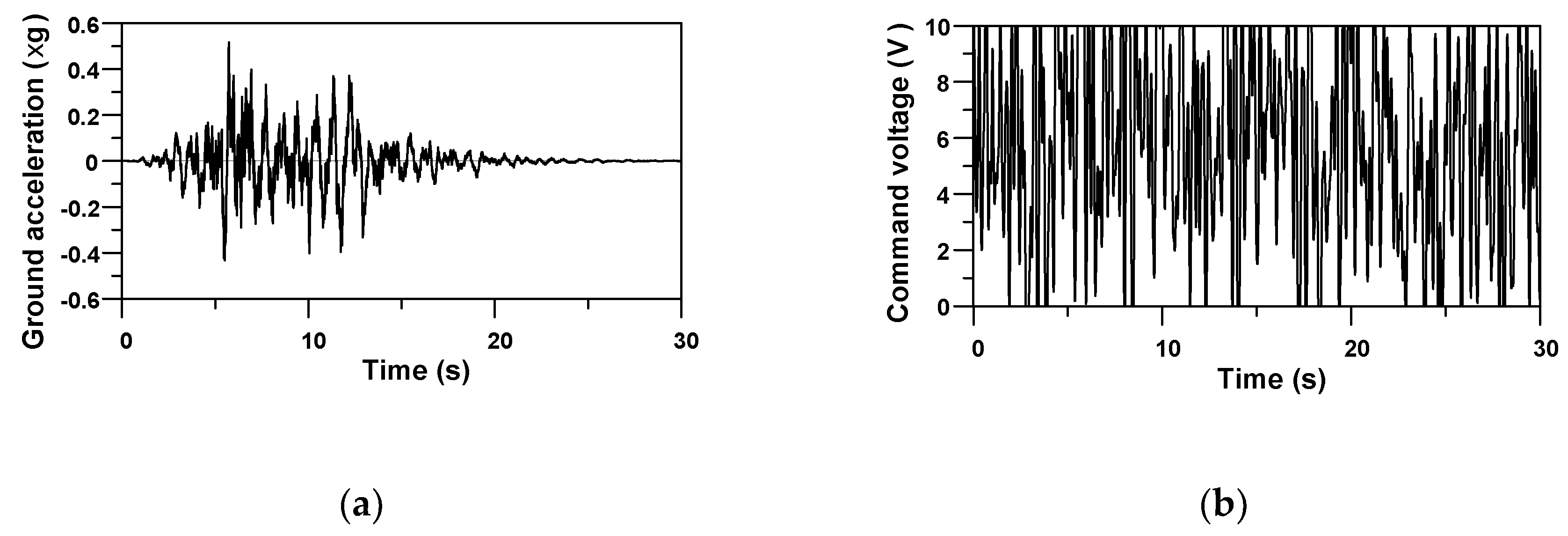
After generating Gaussian white noise with a time-step of 0.005 s and PGA of 0.7× g, the signal was filtered by passing it through the shaping filter, to give the filtered signal the characteristics of realistic earthquakes. The envelope presented in previous study [38] was used to make a more practical ground motion. Figure 6a shows one (EQ No. 6 in Table 2) of the developed seven artificial earthquakes. Inputs of training and verification data included the command voltage for the MR damper, as well as ground motions. For generation of the random command voltage data with the time-step of 0.005 s, a series of 6000 random numbers were generated to have a duration of 30 s between (−1 and 1). The data were shifted and scaled to be within the range (0 to 10), because the saturation limit for the MR damper was set to 10 V. If the identical command voltage data is repeatedly used for training and verification process, the RNN model may overfit the voltage data. Therefore, 13 different voltage time history data were generated for the 10 training data and three verification data, respectively. Figure 6b shows one command voltage time history out of the 13 data. The 13 ground motions in Table 2 and random voltage data were applied to the FE model of the structure and the Bouc–Wen model of the MR damper, and state–space analysis was performed to calculate the seismic responses of Examples 1 and 2. Two calculated responses of Example 1, i.e., the 11th story displacement and acceleration, were used as target output values in the development of the RNN model. Four seismic responses selected as outputs in Figure 5b were used as target values for the Example 2 RNN model.
5. Performance Evaluation of the RNN Simulation Model
The weights and biases of the RNN model were optimized using the training dataset for 1000 epochs in this study. Because each earthquake in Table 2 had 6000 time-steps for a duration of 30 s, one epoch for RNN model training had 60,000 data points. Because the data were too numerous to feed to the computer at once, the training dataset of 60,000 points was divided into batches of 6000, then it took 10 iterations to complete 1 epoch. Each iteration means the training for each earthquake. The weights and biases of the RNN model were updated at the end of every iteration, to fit them to the training data given. All numerical simulations for training the RNN model were implemented using Python 3.5.0 and Tensorflow 1.6.0.
In the context of an optimization algorithm, the function used to evaluate a candidate solution (i.e., in this study, a set of weights and biases for RNN) is referred to as the objective function. In neural networks, the objective function is typically referred to as a loss function, and the value calculated by the loss function is referred to as simply the ‘loss’. The RNN model is trained using an optimization process that requires a loss function to calculate the model error. The model error is usually calculated by matching the target (actual) values and predicted values by the RNN. The target values of the RNN model were the seismic responses of the FE model with the Bouc–Wen model, as explained in the previous section. The two implemented RNN models utilized in this study used the sum of squared errors as the loss function to be minimized for the training process. The root mean squared error (RMSE), which is a commonly used metric to evaluate forecast accuracy, was employed to verify the trained RNN model. The error measures are defined as follows:
where, n is the number of data (i.e., number of time-steps), pi is the predicted responses of the RNN model, and yi is the target responses of the FE model.
Hyperparameter tuning and the selection of a proper function are challenging tasks to develop the accurate RNN model for time series data prediction. Table 3 lists the default hyperparameter values and function used for training and evaluation of the RNN simulation model. Long Short-Term Memory networks (LSTM) [39], which are a special kind of RNN, were used. They work tremendously well on a large variety of problems, due to their capability of learning long-term dependencies, and are now widely used. The hyperbolic tangent (indicated by tanh) was used as the default activation function of the LSTM RNN model. The optimization algorithm employed was the Adam optimizer with a learning rate of 0.01. The Adam optimizer is a popular optimization algorithm in the field of deep learning, because it achieves good results fast compared to the classical stochastic gradient descent procedure.
An issue to be considered with the RNN model is that it can easily overfit training data, resulting in reduction of its predictive capacity. When the RNN model is trained, it can be used to simulate having a large number of different network architectures, by randomly dropping out nodes. This is termed ‘dropout’, and offers a very computationally cheap and remarkably effective regularization method to reduce overfitting and improve the RNN model performance. The dropout rate of 1.0 means no dropout, while 0.0 means no outputs from the layer. A good value for dropout is known to be between (0.5 and 0.8). In this paper, the dropout rate of 0.8 was used in the training process, while 1.0 was used in the verification process. Increasing the number of LSTM cells increases the representational performance of the RNN model, yet makes it prone to overfitting. One LSTM cell was used for the RNN model, because it was sufficient to predict the seismic responses of the examples considered in this study.
The aim of RNN is to detect dependencies in sequential data. This means RNN intends to find correlations between different points within the seismic response time histories. Finding such dependencies makes it possible for RNN to recognize patterns in sequential data and use this information to predict a trend. An appropriate sequence length of the input data needs to be selected to make RNN effectively predict seismic responses. However, there is no rule to determine a feasible sequence length. This value totally depends on the nature of the training and verification data, and the inner correlations. In this paper, in order to find a proper sequence length of input, the RNN model for Example 1 was evaluated by changing the sequence length. The default hyperparameter values in Table 3 except sequence length were used for training and verification of the RNN model. After all the simulations were completed, Table 4 lists the loss and RMSE values to investigate the effect of sequence length on the accuracy of the RNN model. Because there was a deviation in the errors of the RNN model in each epoch, the average of loss and RMSE values of the last 10 epochs are presented. Pearson’s correlation coefficients (CC) are also presented in Table 4 to investigate the relationship between the FEM and RNN models. Pearson’s correlation coefficient is the covariance of the two variables divided by the product of their standard deviations. A correlation coefficient of 1 means that two variables are perfectly positively related. Table 4 shows that as the sequence length increased, both errors of training and verification data decreased until 6, but they increased after that. This means that too long a sequence length actually worsens the prediction performance of the RNN model. This is probably because it is difficult for the RNN model to find the correlations between different points in sequential data that are too lengthy. This phenomenon can be found in the correlation coefficients. The correlation coefficients between the FEM and RNN models increased until the sequence length of 6, but they decreased after that.
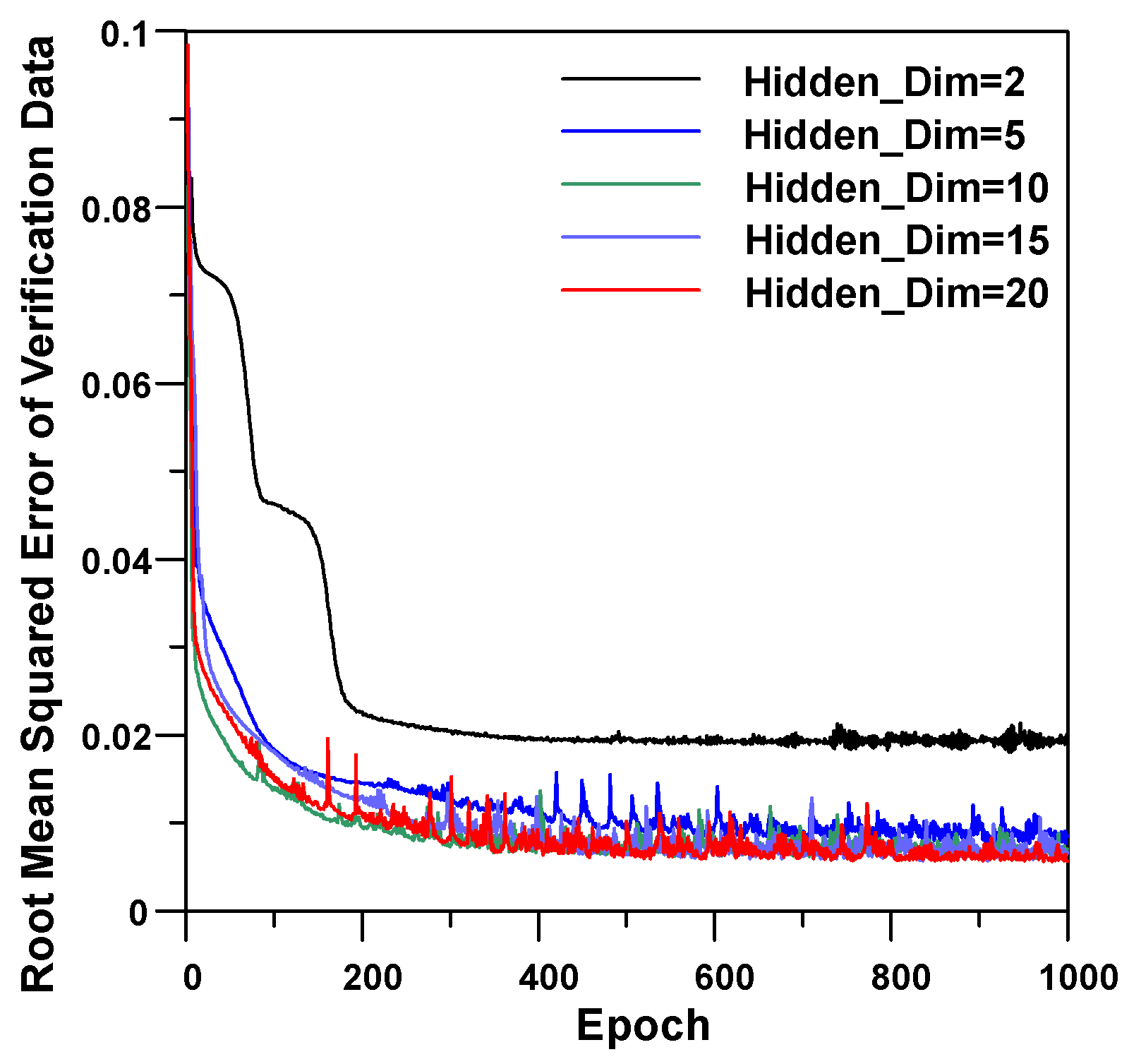
The hidden layer size is a very important hyperparameter that affects the prediction performance of the RNN model. However, optimization of the number of hidden layers remains one of the difficult tasks in the design of the RNN model. Setting too few or too many hidden layers causes high training errors or high generalization errors, respectively. Table 5 lists the average loss and RMSE values of the last 10 epochs, by changing the number of hidden layers. The value of average loss of the training process was consistently reduced as the hidden layer size increased. The value of the average RMSE of the verification process decreased until the hidden layer size of 20, but after that it increased as the hidden layer size increased. If the RNN model size is too large, the model may become overtrained on the training data, and begin to memorize it. This is also termed ‘overfitting’, which is defined as the ability to produce correct results for the training data, while being unable to generalize data that has not been seen before. Table 5 shows that overfitting occurred when the hidden layer size of the RNN model for Example 1 was greater than 20. Therefore, the hidden layer size of 20 was selected for the RNN model of Example 1. Despite the value of the average RMSE having increased after the hidden layer size of 20, the correlation coefficients between the FEM and RNN models continuously increased. However, the increment of the average correlation coefficients gradually decreased with the increment of the hidden layer size.
The simulation results show that compared to the sequence length, the size of the hidden layer had a greater effect on the accuracy of the RNN prediction model. Figure 7 presents the RMSE variation of the verification data according to epoch. When the size of the hidden layer was greater than 10, similar results could be seen in the figure. After about 500 training epochs, the RMSE values of the RNN model with more than 10 hidden layers were hardly changed.
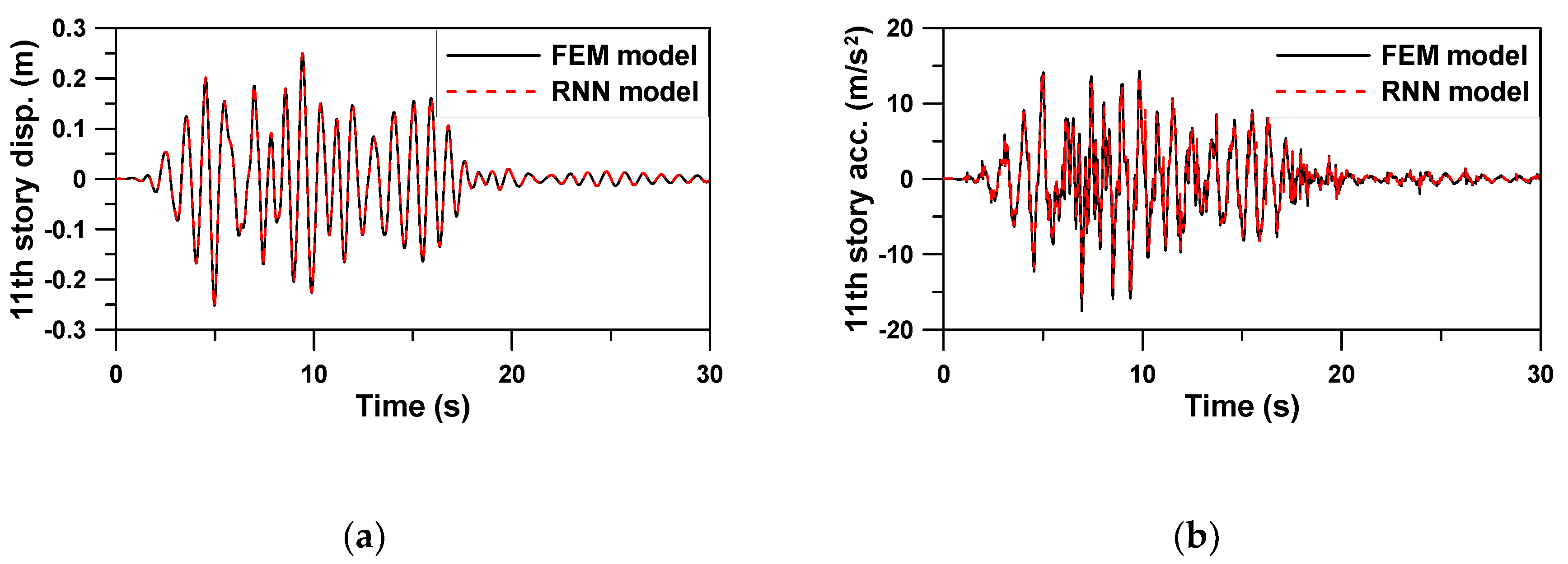
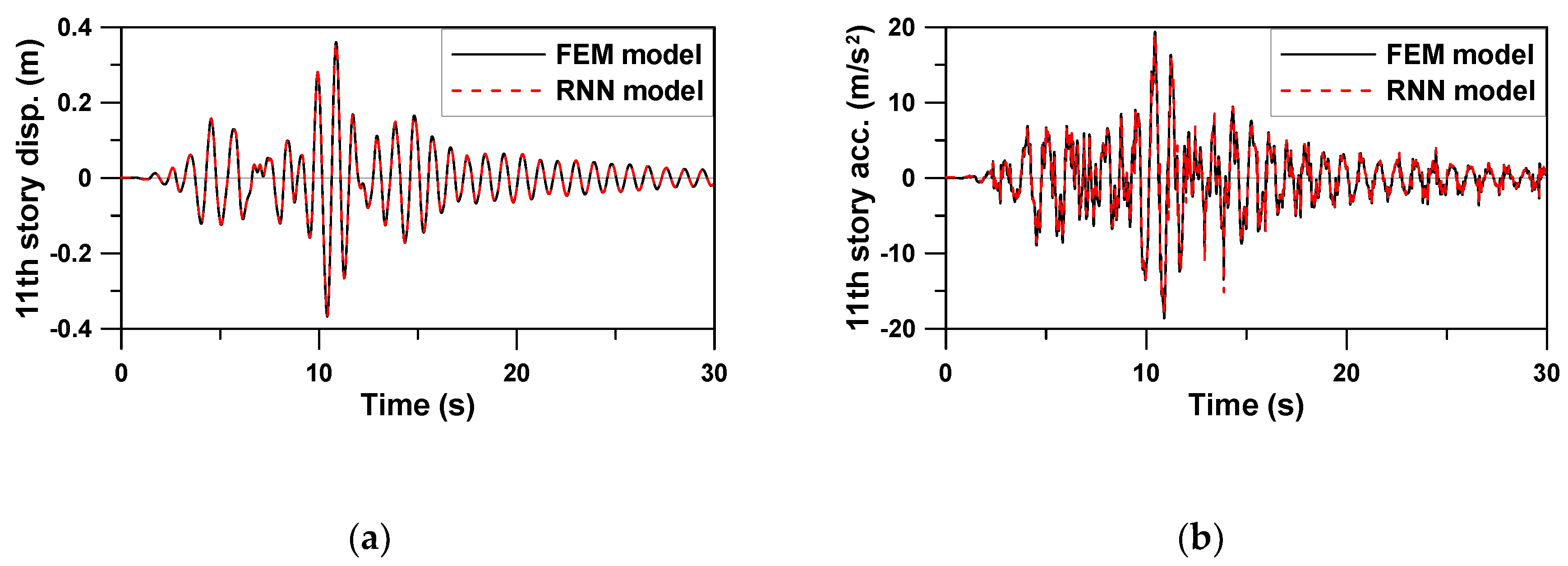
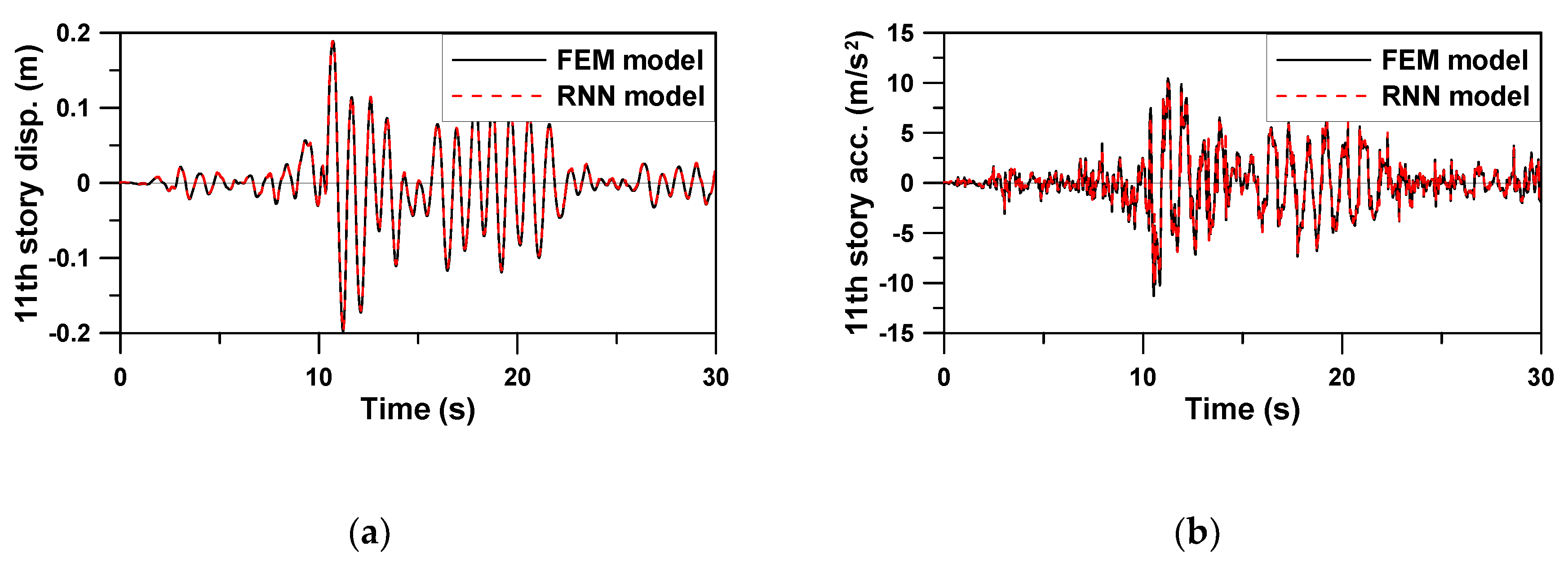
The three most common types of recurrent neural networks are vanilla RNN, LSTM, and gated recurrent units (GRU) [30]. The simulation results of Example 1 show that the errors of the LSTM and GRU RNN models were almost similar, presenting an accuracy that was improved by about 6% compared to Vanilla RNN. In order to evaluate the prediction performance of the trained RNN model, Figure 8, Figure 9 and Figure 10 compare the predicted seismic response time histories of verification data with those of the FE model. The hyperparameter values and functions in Table 3 were used to evaluate the RNN model, except the hidden layer size of 20. Three earthquake loads and command voltages that were not used for training were applied to the trained RNN model. The average RMSE value for all the six seismic responses, i.e., displacement and acceleration responses due to three earthquakes, was calculated to be the very small value of 6.053 × 10⁻³. It can be seen from the time history graphs that the RNN model could very accurately predict not only the displacement response in a relatively smooth curve, but also the rapidly changing acceleration response.
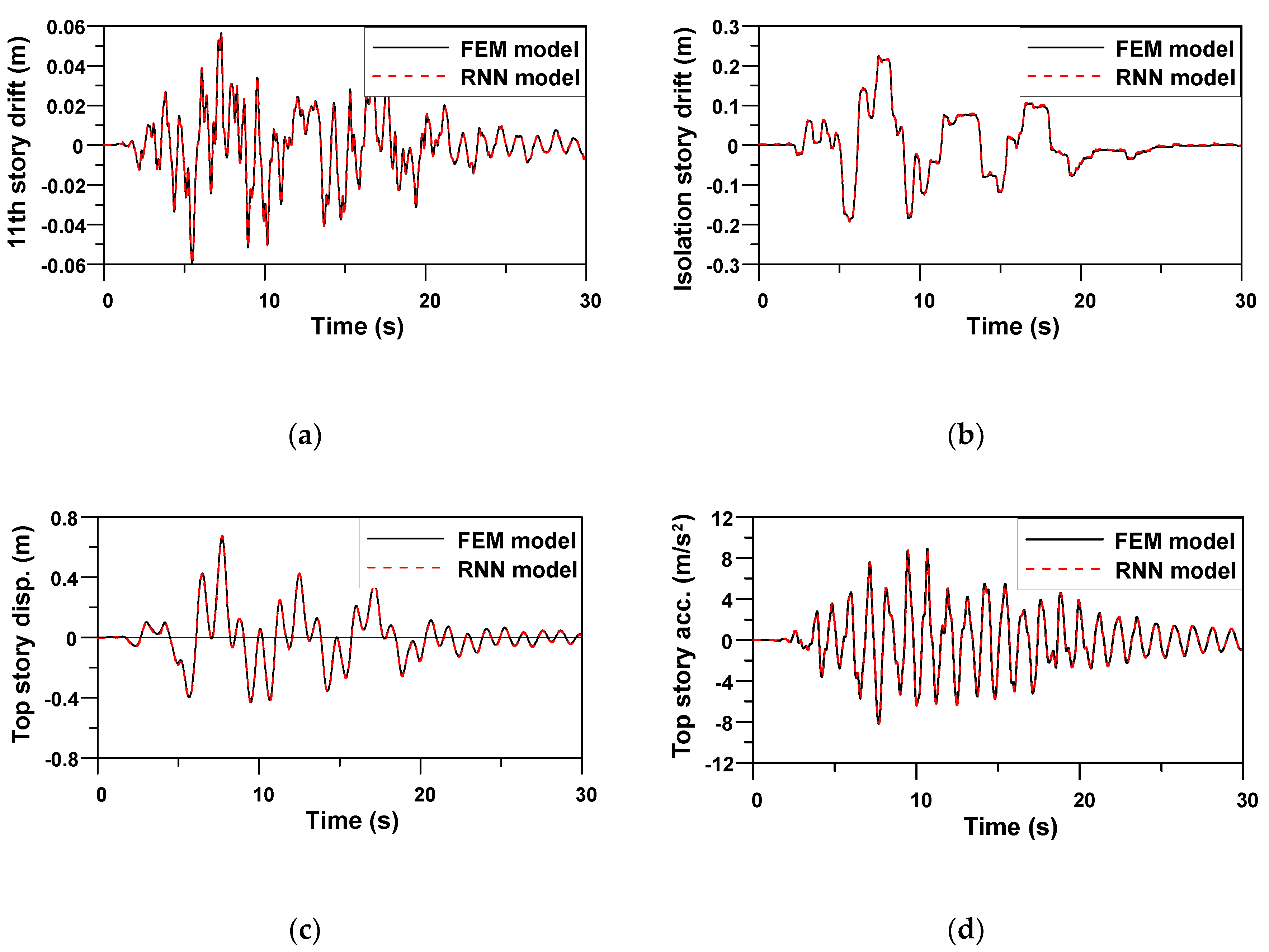
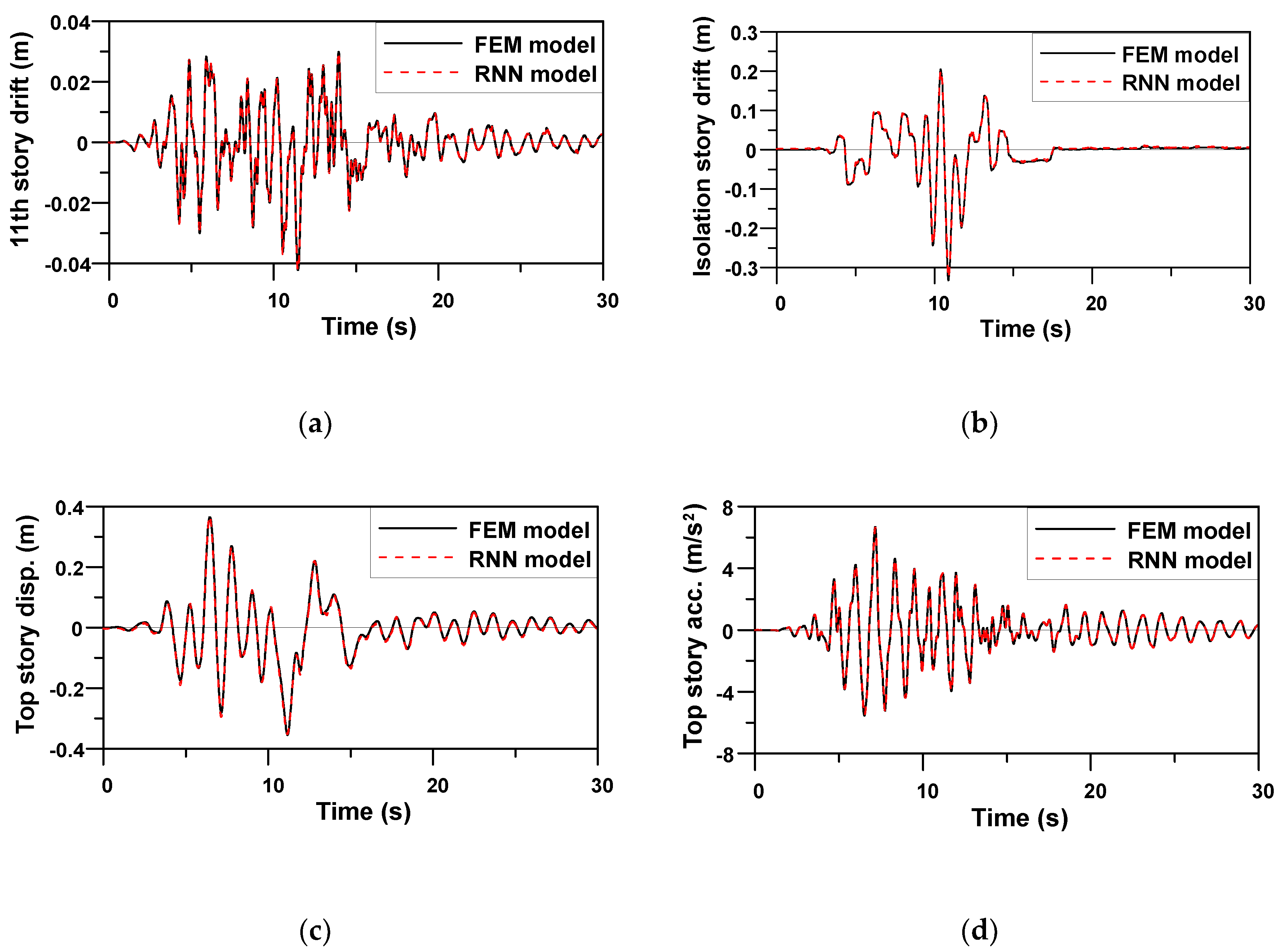
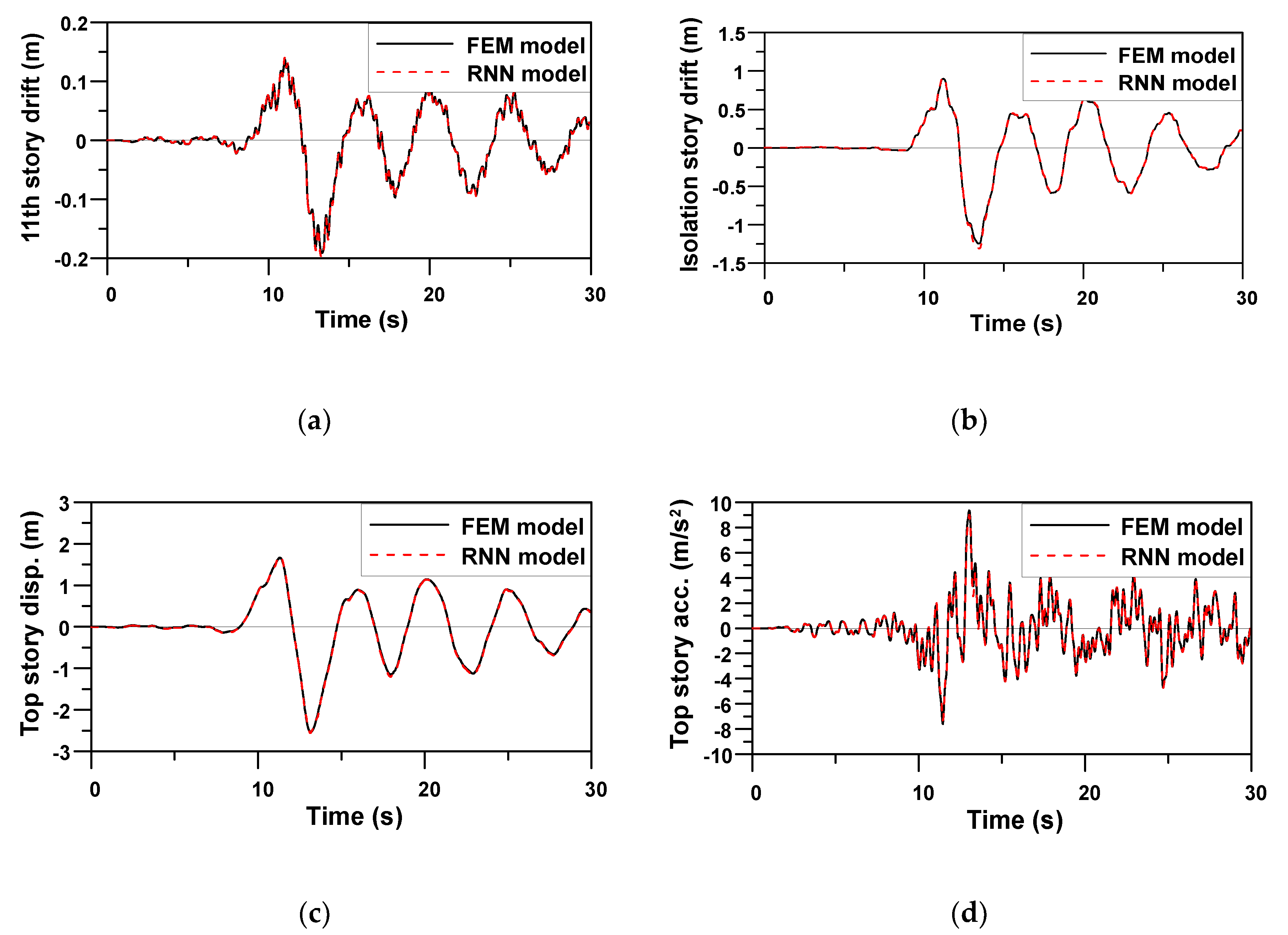
The same hyperparameter values and functions applied to Example 1 were used to evaluate the prediction performance of the RNN model trained for Example 2. Because the outputs of the RNN model for Example 2 were four seismic responses, Figure 11, Figure 12 and Figure 13 compare four response time histories predicted by the RNN model with those of the FE model. It is evident that the predicted responses were very close to the target responses of the FE model. Note that the trained RNN model shows a stable prediction performance for ground motions having different characteristics, despite the peak top story displacement of Jiji earthquake (1999), i.e., the verification earthquake No. 13, being almost 10 times greater than that of the other two artificial earthquakes, i.e., the verification earthquakes Nos. 11 and 12. The average RMSE values for four seismic responses of three verification data from EQ No. 11–13 in Table 2 were 1.232 × 10⁻³, 1.103 × 10⁻³ and 5.249 × 10⁻³, respectively.
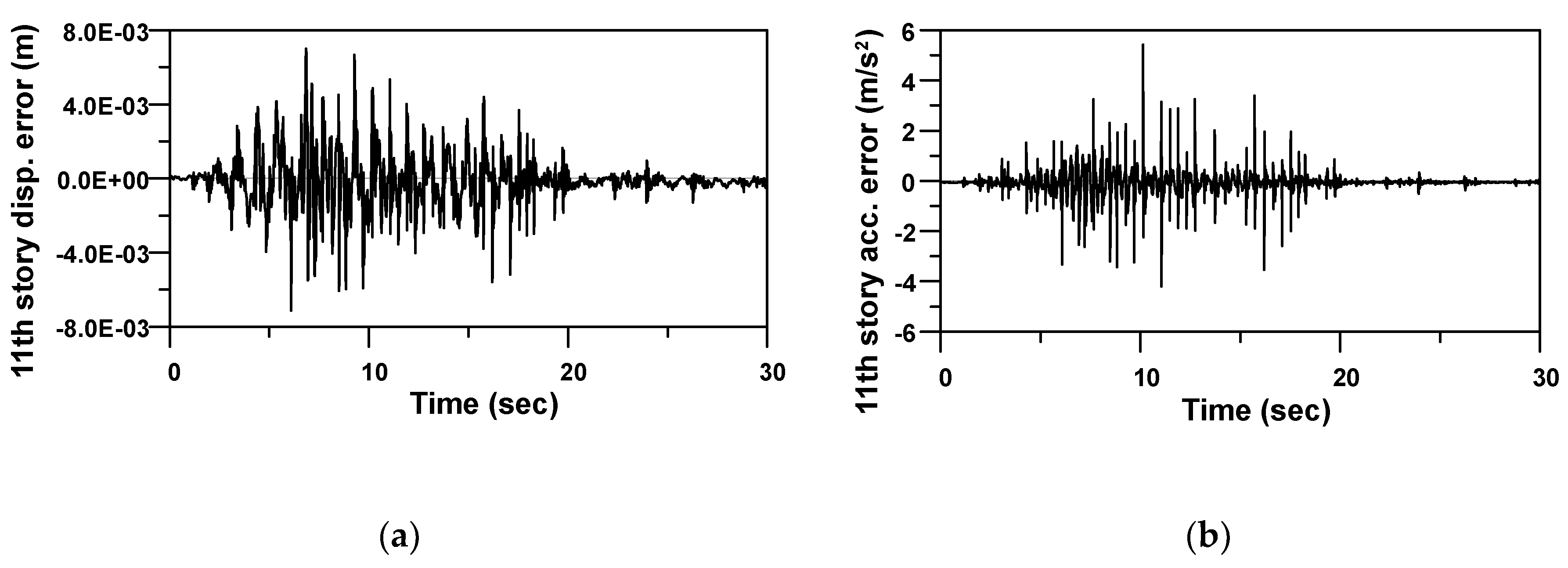
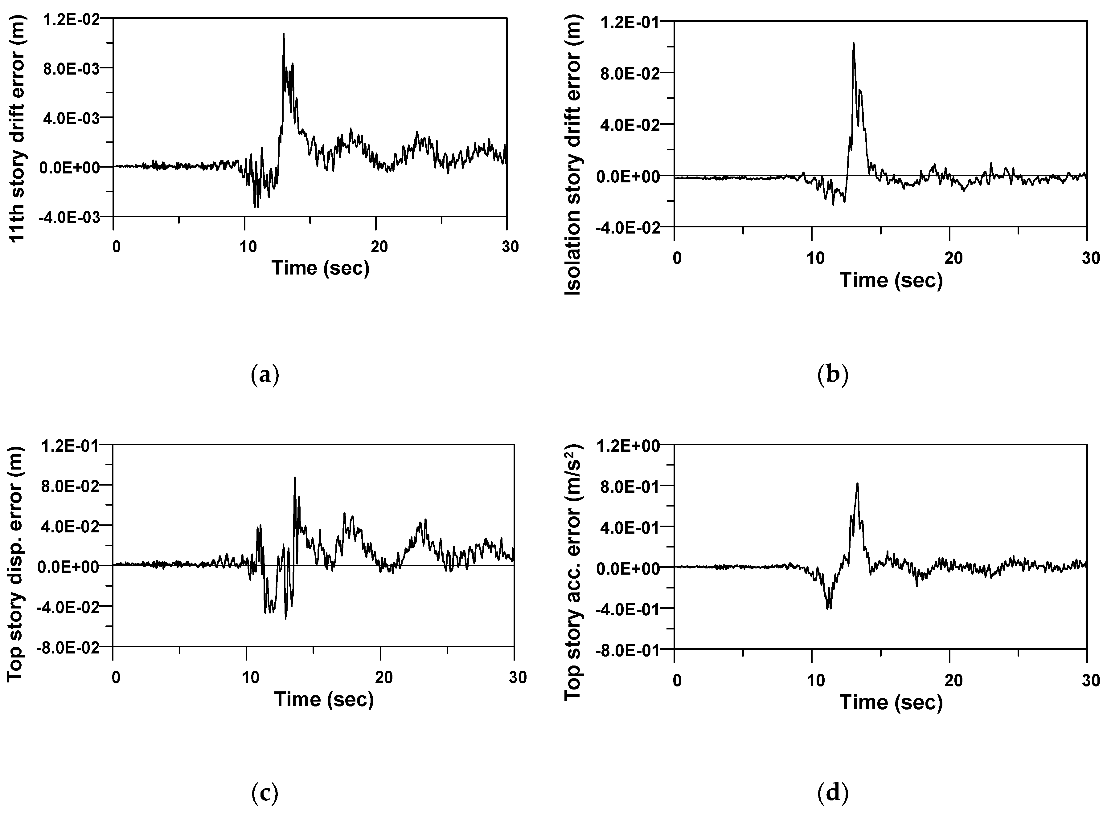
In order to grasp the difference between the FE model and the RNN model more closely, the response errors between two models, namely the FE model responses minus the RNN model responses, were calculated. The response difference time histories between the FE model and the RNN model for Example 1 subjected to an artificial ground motion are presented in Figure 14. Figure 15 shows the different time histories of four outputs of Example 2 subjected to a historical earthquake. It can be seen from the figures that the differences between the FE model and the RNN model increase when the seismic responses of the structure increase. Root Mean Square Error (RMSE) is the standard deviation of the prediction errors. Because the peak responses in the seismic analysis are very important values for the structural design process, it would be desirable that the objective function for optimization of the RNN model should consider not only the commonly used RMSE but also the maximum prediction errors.
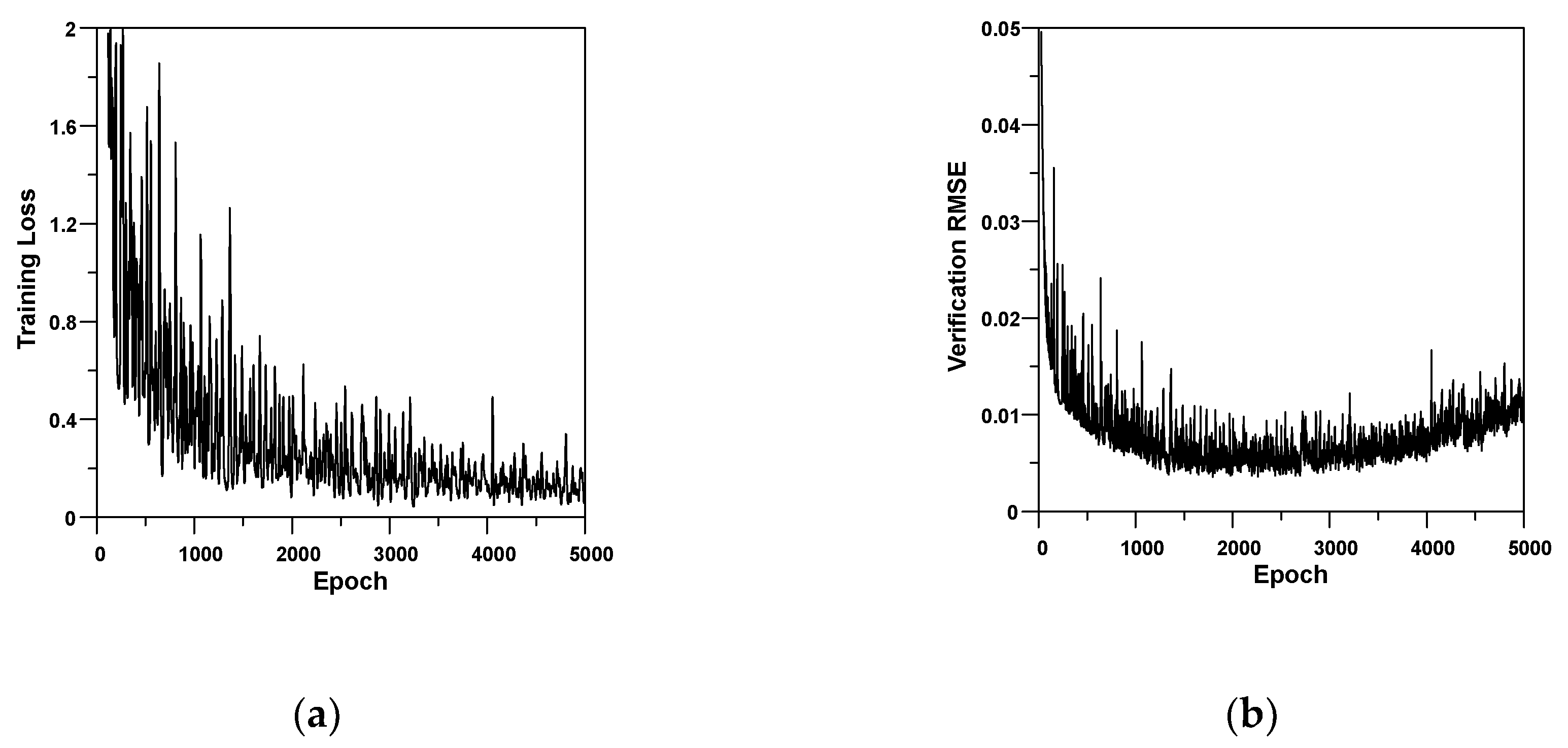
Figure 16 shows the variation of loss and RMSE values according to epoch for Example 2. The wiggle shown in the loss and RMSE graphs is usually related to the batch size. When the batch size is the full dataset, the wiggle will be minimal. The figure represents that the loss of training process consistently decreased. On the other hand, the RMSE value decreased until about 2000 epochs, but increased after that. This means that overfitting started at around 2000 epochs. Therefore, variation of the verification error should be monitored to avoid overfitting of the RNN model.
The averages of computational times for 10 simulation runs of the FE model were 23.38 and 45.87 s for Examples 1 and 2, respectively. If the time-step of numerical integration is too large, the nonlinear equation solver fails to converge. Therefore, the time-step of 0.001 s, which was the maximum time-step for stable analyses of all the ground motions, was employed for FE model analysis using Matlab. The computational times of 0.0130 and 0.0142 s for Examples 1 and 2, respectively, were calculated from the average of 10 simulation runs for the RNN model. The ratios of simulation time of the RNN model to the FE model were 0.06 and 0.03% for Examples 1 and 2, respectively. Compared to the FE model, the RNN model could greatly reduce simulation time, and provide very accurate results. Because the computational time difference between the RNN models was trivial, the larger the FE model, the more effective the RNN model. When designing a control algorithm for a semi-active control system, it is necessary to perform many numerical simulations. Using the RNN model, the simulation runs of 1798 and 3230 for Examples 1 and 2, respectively, could be carried out; while using the FE model, only one simulation could be executed. This means that when a soft computing-based optimization algorithm is applied to the design of a semi-active control system, the RNN model can allow a far larger search area to be explored. Therefore, the proposed RNN model can be an efficient means for the numerical simulation of a building structure with a semi-active control system. A personal computer with Intel® Core™ i7-7500U CPU and 8 GB RAM was employed in this study.
6. Conclusions
This study developed an RNN model for the seismic response simulation of a building structure with a semi-active control system. An 11-story building with a semi-active TMD and a 26-story building with a semi-active mid-story isolation system were used as example structures. A magnetorheological damper was used as the semi-active control devices for both example structures. Training and verification dataset were generated using historical and artificial earthquakes. A series of numerical simulations were performed to investigate the effect of hyperparameters on the prediction accuracy of the RNN model. It was found that the sequence length and the hidden layer size mainly influenced the accuracy of the RNN model, especially the hidden layer size, which turned out to be the most important hyperparameter. The other hyperparameters and functions did not considerably affect the prediction performance of the RNN model. In general, a longer sequence length increases the accuracy of the RNN model. However, too long a sequence length worsens the prediction performance of the RNN model, because it makes the RNN model confuse the correlations between different points in too lengthy time series data. A too large hidden layer size may result in overfitting; thus, attention needs to be paid to appropriately adjusting the hidden layer size. Compared to the FE model, the well trained RNN model very accurately predicted the seismic responses of the building with a semi-active control system. As the simulation time of the RNN model was extremely reduced, thousands of simulation runs of the RNN model could be conducted during only one simulation run of the FE model. The simulation results show that the size of the example structure has little effect on the accuracy of the RNN prediction model. Because the computational time of the RNN models is trivial compared to the FE model, the larger the size of the structure is, the more effective the RNN model is. The author believes that the RNN model developed in this study can be very useful for the numerical simulation and development of a building structure with a semi-active control system. Moreover, future studies are expected to apply the proposed RNN model to the optimal design of control algorithms for a semi-active control system.
Author Contributions
The author has read and agreed to the published version of the manuscript.
Funding
This research was supported by a National Research Foundation of Korea (NRF) grant, funded by the Korea government (MEST), grant number NRF-2019R1A2C1002385.
Conflicts of Interest
The author declares no conflict of interest.
References
- Bitaraf, M.; Ozbulut, O.E.; Hurlebaus, S.; Barroso, L. Application of semi-active control strategies for seismic protection of buildings with MR dampers. Eng. Struct. 2010, 32, 3040–3047. [Google Scholar] [CrossRef]
- Karami, K.; Manie, S.; Ghafouri, K.; Nagarajaiah, S. Nonlinear structural control using integrated DDA/ISMP and semi-active tuned mass damper. Eng. Struct. 2019, 181, 589–604. [Google Scholar] [CrossRef]
- Soto, M.G.; Adeli, H. Semi-active vibration control of smart isolated highway bridge structures using replicator dynamics. Eng. Struct. 2019, 186, 536–552. [Google Scholar] [CrossRef]
- Chey, M.H.; Chase, J.G.; Mander, J.B.; Carr, A.J. Semi-active tuned mass damper building systems: Application. Earthq. Eng. Struct. Dyn. 2010, 39, 69–89. [Google Scholar] [CrossRef]
- Kang, J.W.; Kim, H.S.; Lee, D.G. Mitigation of wind response of a tall building using semi-active tuned mass dampers. Struct. Des. Tall Spec. 2011, 20, 552–565. [Google Scholar] [CrossRef]
- Kim, H.S.; Kang, J.W. Optimal design of smart mid-story isolated control system for a high-rise building. Int. J. Steel Struct. 2019, 19, 1988–1995. [Google Scholar] [CrossRef]
- Bani-Hani, K.A.; Sheban, M.A. Semi-active neuro-control for base-isolation system using magnetorheological (MR) dampers. Earthq. Eng. Struct. Dyn. 2006, 35, 1119–1144. [Google Scholar] [CrossRef]
- Kim, H.S.; Kang, J.W. Smart outrigger damper system for response reduction of tall buildings subjected to wind and seismic excitations. Int. J. Steel Struct. 2017, 17, 1263–1272. [Google Scholar] [CrossRef]
- Christenson, R.E.; Spencer, B.F.; Johnson, E.A. Semiactive connected control method for adjacent multidegree-of-freedom buildings. J. Eng. Mech. 2007, 133, 290–298. [Google Scholar] [CrossRef]
- Bhaiya, V.; Shrimali, M.K.; Bharti, S.D.; Datta, T.K. Modified semiactive control with MR dampers for partially observed systems. Eng. Struct. 2019, 191, 129–147. [Google Scholar] [CrossRef]
- Symans, M.D.; Constantinou, M.C. Semi-active control systems for seismic protection of structures: A state-of-the-art review. Eng. Struct. 1999, 21, 469–487. [Google Scholar] [CrossRef]
- Jansen, L.M.; Dyke, S.J. Semi-active control strategies for MR dampers: A comparative study. J. Eng. Mech. 2000, 126, 795–803. [Google Scholar] [CrossRef] [Green Version]
- Oliveira, F.; Morais, P.; Suleman, A. A comparative study of semi-active control strategies for base isolated buildings. Earthq. Eng. Eng. Vib. 2015, 14, 487–502. [Google Scholar] [CrossRef]
- Kim, H.S.; Kang, J.W. Semi-active fuzzy control of a wind-excited tall building using multi-objective genetic algorithm. Eng. Struct. 2012, 41, 242–257. [Google Scholar] [CrossRef]
- Uz, M.E.; Hadi, M.N.S. Optimal design of semi active control for adjacent buildings connected by MR damper based on integrated fuzzy logic and multi-objective genetic algorithm. Eng. Struct. 2014, 69, 135–148. [Google Scholar] [CrossRef] [Green Version]
- Ohtori, Y.; Christenson, R.E.; Spencer, B.F.; Dyke, S.J. Benchmark control problems for seismically excited nonlinear buildings. J. Eng. Mech. 2004, 130, 366–385. [Google Scholar] [CrossRef] [Green Version]
- Salehi, H.; Burgueño, R. Emerging artificial intelligence methods in structural engineering. Eng. Struct. 2018, 171, 170–189. [Google Scholar] [CrossRef]
- Saka, M.P.; Geem, Z.W. Mathematical and metaheuristic applications in design optimization of steel frame structures: An extensive review. Math. Probl. Eng. 2013, 2013, 271031. [Google Scholar] [CrossRef] [Green Version]
- Karimi, I.; Khaji, N.; Ahmadi, M.; Mirzayee, M. System identification of concrete gravity dams using artificial neural networks based on a hybrid finite element–boundary element approach. Eng. Struct. 2010, 32, 3583–3591. [Google Scholar] [CrossRef]
- Alves, V.; Cury, A.; Roitman, N.; Magluta, C.; Cremona, C. Structural modification assessment using supervised learning methods applied to vibration data. Eng. Struct. 2015, 99, 439–448. [Google Scholar] [CrossRef]
- Wang, Q.; Wang, J.; Huang, X.; Zhang, L. Semiactive nonsmooth control for building structure with deep learning. Complexity 2017, 2017, 6406179. [Google Scholar] [CrossRef] [Green Version]
- Manevitz, L.M.; Yousef, M.; Givoli, D. Finite–element mesh generation using self–organizing neural networks. Comput. Aided Civ. Inf. 2002, 12, 233–250. [Google Scholar] [CrossRef]
- Kim, H.S.; Roschke, P.N.; Lin, P.Y.; Loh, C.H. Neuro-fuzzy model of hybrid semi-active base isolation system with FPS bearings and an MR damper. Eng. Struct. 2006, 28, 947–958. [Google Scholar] [CrossRef]
- Xia, P.Q. An inverse model of MR damper using optimal neural network and system identification. J. Sound Vib. 2003, 266, 1009–1023. [Google Scholar] [CrossRef]
- The Unreasonable Effectiveness of Recurrent Neural Networks. Available online: http://karpathy.github.io/2015/05/21/rnn-effectiveness/ (accessed on 3 April 2020).
- Understanding LSTM Networks. Available online: https://colah.github.io/posts/2015-08-Understanding-LSTMs/ (accessed on 3 April 2020).
- Kim, H.S.; Roschke, P.N. Design of fuzzy logic controller for smart base isolation system using genetic algorithm. Eng. Struct. 2006, 28, 84–96. [Google Scholar] [CrossRef]
- Ok, S.Y.; Kim, D.S.; Park, K.S.; Koh, H.M. Semi-active fuzzy control of cable-stayed bridges using magneto-rheological dampers. Eng. Struct. 2007, 29, 776–788. [Google Scholar] [CrossRef]
- Kim, H.S.; Kang, J.W. Multi-objective fuzzy control of smart base isolated spatial structure. Int. J. Steel Struct. 2014, 14, 547–556. [Google Scholar] [CrossRef]
- Zalewski, R.; Nachman, J.; Shillor, M.; Bajkowski, J. Dynamic model for a magnetorheological damper. Appl. Math. Model. 2014, 38, 2366–2376. [Google Scholar] [CrossRef]
- Spencer, B.F.; Dyke, S.J.; Sain, M.K.; Carlson, J.D. Phenomenological model of a magnetorheological damper. J. Eng. Mech. 1997, 123, 230–238. [Google Scholar] [CrossRef]
- Duchanoy, C.A.; Moreno-Armendáriz, M.A.; Moreno-Torres, J.C.; Cruz-Villar, C.A. A deep neural network based model for a kind of magnetorheological dampers. Sensors 2019, 19, 1333. [Google Scholar] [CrossRef] [Green Version]
- Bathaei, A.; Zahrai, S.M.; Ramezani, M. Semi-active seismic control of an 11-DOF building model with TMDþMR damper using type-1 and -2 fuzzy algorithms. J. Vib. Cotrol 2018, 24, 2938–2953. [Google Scholar] [CrossRef]
- Sueoka, T.; Torii, S.; Tsuneki, Y. The application of response control design using middle-story isolation system to high-rise building. In Proceedings of the 13th World Conference on Earthquake Engineering, Vancouver, BC, Canada, 1–6 August 2004. [Google Scholar]
- Yi, F.; Dyke, S.J.; Caicedo, J.M.; Carlson, J.D. Experimental verification of multi-input seismic control strategies for smart dampers. J. Eng. Mech. 2001, 127, 1152–1164. [Google Scholar] [CrossRef] [Green Version]
- Alotta, G.; Paola, M.D.; Pirrotta, A. Fractional Tajimi–Kanai model for simulating earthquake ground motion. Bull. Earthq. Eng. 2014, 12, 2495–2506. [Google Scholar] [CrossRef]
- Ramallo, J.C.; Johnson, E.A.; Spencer, B.F. “Smart” base isolation systems. J. Eng. Mech. 2002, 128, 1088–1100. [Google Scholar] [CrossRef] [Green Version]
- Kim, H.S.; Roschke, P.N. GA-fuzzy control of smart base isolated benchmark building using supervisory control technique. Adv. Eng. Softw. 2007, 38, 453–465. [Google Scholar] [CrossRef]
- Hochreiter, S.; Schmidhuber, J. Long short term memory. Neural Comput. 1997, 9, 1735–1780. [Google Scholar] [CrossRef] [PubMed]
Figure 1.
Difference between feedforward and recurrent neural networks: (a) Feedforward neural network; (b) Recurrent neural network.
Figure 1.
Difference between feedforward and recurrent neural networks: (a) Feedforward neural network; (b) Recurrent neural network.

Figure 2.
Various architecture of RNN models: (a) one-to-one; (b) one-to-many; (c) many-to-one; (d) many-to-many.
Figure 2.
Various architecture of RNN models: (a) one-to-one; (b) one-to-many; (c) many-to-one; (d) many-to-many.

Figure 3.
Outline of the seismic response simulation model of a seismic-excited structure with semi-active control system: (a) Conventional model; (b) RNN-based model.
Figure 3.
Outline of the seismic response simulation model of a seismic-excited structure with semi-active control system: (a) Conventional model; (b) RNN-based model.

Figure 4.
Analytical models of example structures: (a) Model with a semi-active tuned mass damper (Example 1); (b) Model with a semi-active mid-story isolation system (Example 2).
Figure 4.
Analytical models of example structures: (a) Model with a semi-active tuned mass damper (Example 1); (b) Model with a semi-active mid-story isolation system (Example 2).

Figure 5.
Input and output data of the RNN model: (a) RNN model for a building with semi-active TMD (Example 1); (b) RNN model for a building with SMIS (Example 2).
Figure 5.
Input and output data of the RNN model: (a) RNN model for a building with semi-active TMD (Example 1); (b) RNN model for a building with SMIS (Example 2).

Figure 6.
Time histories of input data for RNN: (a) Ground acceleration time history of artificial earthquake 1 (EQ No. 6); (b) Command voltage time history.
Figure 6.
Time histories of input data for RNN: (a) Ground acceleration time history of artificial earthquake 1 (EQ No. 6); (b) Command voltage time history.

Figure 7.
RMSE variation versus epoch of RNN model for Example 1.

Figure 8.
Comparison of the time history responses of Example 1 between FEM and RNN models (EQ No. 11): (a) Displacement time history; (b) Acceleration time history.
Figure 8.
Comparison of the time history responses of Example 1 between FEM and RNN models (EQ No. 11): (a) Displacement time history; (b) Acceleration time history.

Figure 9.
Comparison of time history responses of Example 1 between FEM and RNN models (EQ No. 12): (a) Displacement time history; (b) Acceleration time history.
Figure 9.
Comparison of time history responses of Example 1 between FEM and RNN models (EQ No. 12): (a) Displacement time history; (b) Acceleration time history.

Figure 10.
Comparison of time history responses of Example 1 between FEM and RNN models (EQ No. 13): (a) Displacement time history; (b) Acceleration time history.
Figure 10.
Comparison of time history responses of Example 1 between FEM and RNN models (EQ No. 13): (a) Displacement time history; (b) Acceleration time history.

Figure 11.
Comparison of the time history responses of Example 2 between FEM and RNN models (EQ No. 11): (a) 11th story drift time history; (b) Isolation story drift time history; (c) Top story displacement time history; (d) Top story acceleration time history.
Figure 11.
Comparison of the time history responses of Example 2 between FEM and RNN models (EQ No. 11): (a) 11th story drift time history; (b) Isolation story drift time history; (c) Top story displacement time history; (d) Top story acceleration time history.

Figure 12.
Comparison of the time history responses of Example 2 between FEM and RNN models (EQ No. 12): (a) 11th story drift time history; (b) Isolation story drift time history; (c) Top story displacement time history; (d) Top story acceleration time history.
Figure 12.
Comparison of the time history responses of Example 2 between FEM and RNN models (EQ No. 12): (a) 11th story drift time history; (b) Isolation story drift time history; (c) Top story displacement time history; (d) Top story acceleration time history.

Figure 13.
Comparison of the time history responses of Example 2 between FEM and RNN models (EQ No. 13): (a) 11th story drift time history; (b) Isolation story drift time history; (c) Top story displacement time history; (d) Top story acceleration time history.
Figure 13.
Comparison of the time history responses of Example 2 between FEM and RNN models (EQ No. 13): (a) 11th story drift time history; (b) Isolation story drift time history; (c) Top story displacement time history; (d) Top story acceleration time history.

Figure 14.
Response error time histories of Example 1 (EQ No. 11): (a) Displacement error time history; (b) Acceleration error time history.
Figure 14.
Response error time histories of Example 1 (EQ No. 11): (a) Displacement error time history; (b) Acceleration error time history.

Figure 15.
Response error time histories of Example 2 (EQ No. 13): (a) 11th story drift error time history; (b) Isolation story drift error time history; (c) Top story displacement error time history; (d) Top story acceleration error time history.
Figure 15.
Response error time histories of Example 2 (EQ No. 13): (a) 11th story drift error time history; (b) Isolation story drift error time history; (c) Top story displacement error time history; (d) Top story acceleration error time history.

Figure 16.
Error variation versus epoch: (a) Loss variation in training; (b) RMSE variation in verification.
Figure 16.
Error variation versus epoch: (a) Loss variation in training; (b) RMSE variation in verification.


Table 1.
Story mass and stiffness of the example structures.
| 26-Story Model w/SMIS | 11-Story Model w/STMD | |||||||
|---|---|---|---|---|---|---|---|---|
| Story | Mass (kg) | Stiffness (kN/m) | Story | Mass (kg) | Stiffness (kN/m) | Story | Mass (kg) | Stiffness (kN/m) |
| 1 | 3,080,514 | 3.18 × 10⁶ | 14 | 3,186,563 | 2.32 × 10⁶ | 1 | 215,370 | 4.68 × 10⁵ |
| 2 | 2,582,900 | 2.68 × 10⁶ | 15 | 3,140,676 | 2.63 × 10⁶ | 2 | 201,750 | 4.76 × 10⁵ |
| 3 | 1,726,352 | 6.34 × 10⁶ | 16 | 3,132,518 | 2.65 × 10⁶ | 3 | 201,750 | 4.68 × 10⁵ |
| 4 | 1,733,490 | 5.92 × 10⁶ | 17 | 3,125,381 | 2.59 × 10⁶ | 4 | 200,930 | 4.50 × 10⁵ |
| 5 | 1,716,155 | 5.71 × 10⁶ | 18 | 3,170,247 | 2.59 × 10⁶ | 5 | 200,930 | 4.50 × 10⁵ |
| 6 | 1,715,135 | 5.36 × 10⁶ | 19 | 3,168,208 | 2.48 × 10⁶ | 6 | 200,930 | 4.50 × 10⁵ |
| 7 | 1,718,195 | 5.20 × 10⁶ | 20 | 3,117,223 | 2.49 × 10⁶ | 7 | 203,180 | 4.50 × 10⁵ |
| 8 | 1,697,801 | 4.95 × 10⁶ | 21 | 3,094,790 | 2.34 × 10⁶ | 8 | 202,910 | 4.37 × 10⁵ |
| 9 | 1,721,254 | 4.79 × 10⁶ | 22 | 3,084,593 | 2.24 × 10⁶ | 9 | 202,910 | 4.37 × 10⁵ |
| 10 | 3,127,420 | 4.45 × 10⁶ | 23 | 3,076,435 | 2.17 × 10⁶ | 10 | 176,100 | 4.37 × 10⁵ |
| 11 | 3,128,440 | 1.08 × 10⁶ | 24 | 3,447,606 | 2.11 × 10⁶ | 11 | 66,230 | 3.12 × 10⁵ |
| 12 | 4,030,874 | 8.07 × 10⁵ | 25 | 3,461,882 | 1.73 × 10⁶ | - | - | - |
| 13 | 3,567,930 | 3.11 × 10⁶ | 26 | 5,769,463 | 1.51 × 10⁶ | - | - | - |
Table 2.
Earthquakes for the training and verification of RNN.
| No. | EQ Name | PGA 1 | Type | Purpose |
|---|---|---|---|---|
| 1 | El Centro (1940) | 0.313× g | Far-field | Training |
| 2 | Taft (1952) | 0.156× g | Far-field | Training |
| 3 | Northridge (1994) | 0.603× g | Near-field | Training |
| 4 | Loma Prieta (1989) | 0.220× g | Near-field | Training |
| 5 | Kobe (1995) | 0.686× g | Near-field | Training |
| 6 | Artificial EQ1 | 0.517× g | - | Training |
| 7 | Artificial EQ2 | 0.537× g | - | Training |
| 8 | Artificial EQ3 | 0.576× g | - | Training |
| 9 | Artificial EQ4 | 0.566× g | - | Training |
| 10 | Artificial EQ5 | 0.385× g | - | Training |
| 11 | Artificial EQ6 | 0.562× g | - | Verification |
| 12 | Artificial EQ7 | 0.615× g | - | Verification |
| 13 | Jiji (1999) | 0.512× g | Near-field | Verification |
1 Peak ground acceleration (× g).
Table 3.
Default hyperparameter values and function.
| Item | Value |
|---|---|
| Sequence length | 5 |
| RNN cell number | 1 |
| Dropout rate | 0.8 |
| Hidden layer dimension | 5 |
| Learning rate | 0.01 |
| RNN type | LSTM |
| Activation function | tanh |
| Optimizer | Adam |
Table 4.
Effect of sequence length on accuracy.
| Sequence Length | Average Loss | Average RMSE | Average CC |
|---|---|---|---|
| 1 | 2.648 | 11.490 × 10⁻³ | 0.988597 |
| 2 | 2.317 | 9.408 × 10⁻³ | 0.995088 |
| 5 | 2.273 | 8.623 × 10⁻³ | 0.995840 |
| 6 | 2.248 | 8.141 × 10⁻³ | 0.995981 |
| 7 | 2.496 | 8.925 × 10⁻³ | 0.995625 |
| 10 | 2.535 | 9.279 × 10⁻³ | 0.995115 |
Table 5.
Effect of the hidden layer size on accuracy.
| Hidden Layer Size | Average Loss | Average RMSE | Average CC |
|---|---|---|---|
| 2 | 6.207 | 19.516 × 10⁻³ | 0.974948 |
| 5 | 2.263 | 8.509 × 10⁻³ | 0.995678 |
| 10 | 1.278 | 6.733 × 10⁻³ | 0.996786 |
| 15 | 1.004 | 6.561 × 10⁻³ | 0.996964 |
| 20 | 0.769 | 6.053 × 10⁻³ | 0.997070 |
| 30 | 0.618 | 6.341 × 10⁻³ | 0.997119 |
| 40 | 0.539 | 6.757 × 10⁻³ | 0.997185 |
© 2020 by the author. Licensee MDPI, Basel, Switzerland. This article is an open access article distributed under the terms and conditions of the Creative Commons Attribution (CC BY) license (http://creativecommons.org/licenses/by/4.0/).
Share and Cite
MDPI and ACS Style
Kim, H.-S. Development of Seismic Response Simulation Model for Building Structures with Semi-Active Control Devices Using Recurrent Neural Network. Appl. Sci. 2020, 10, 3915. https://doi.org/10.3390/app10113915
AMA Style
Kim H-S. Development of Seismic Response Simulation Model for Building Structures with Semi-Active Control Devices Using Recurrent Neural Network. Applied Sciences. 2020; 10(11):3915. https://doi.org/10.3390/app10113915
Chicago/Turabian StyleKim, Hyun-Su. 2020. "Development of Seismic Response Simulation Model for Building Structures with Semi-Active Control Devices Using Recurrent Neural Network" Applied Sciences 10, no. 11: 3915. https://doi.org/10.3390/app10113915
Note that from the first issue of 2016, this journal uses article numbers instead of page numbers. See further details here.