Optimizing Replaced Nozzle Diameter of Abrasive Blasting Systems Using Experiment Technique Design

Abstract

The blasting technique has been broadly utilized to prepare new surfaces for painting, engraving, etc., in industry. In fact, the minimization of the cleaning cost system is essential. However, the knowledge of this technique in terms of optimization has been poor so far. The aim of this study is to find the optimum replaced boron carbide nozzle diameter for the abrasive blasting system. The basis of the study is to find the replaced nozzle diameter to minimize the cost of the blasting system. Seven main parameters are adopted for examining their influences on the response and the optimum replaced nozzle diameter. The design of experiment (DOE) technique is utilized by using Minitab^@19. The results reveal that the initial nozzle diameter has the strongest impact on the optimum replaced nozzle diameter. Furthermore, the proposed regression model has been found to be entirely insistent to the experiments. The utilization of this model can provide an effective way to simplify the calculation of the optimum initial nozzle diameter for boron carbide.

1. Introduction

Abrasive blasting systems have been widely utilized for cleaning surfaces which could be needed for the further steps such as repairing, painting, welding, engraving, coating, etc. In addition, they are extensively used with various types of abrasive materials such as copper slag, steel shot, sand, etc. Although the blasting technology exhibits weaknesses like the emission of dust which can be inhaled by the operators [1], it is still used in industry due to its huge advantages. According to [2], the world’s demand for abrasives increased from $8.6 billion in 2014 to $11.4 billion in 2019. This proves that the demand for abrasive blasting is huge. Accordingly, the reduction of the blasting cost is crucially important. However, there has been little research related to this topic. Vu et al. [3] investigated the influences of six parameters (the initial nozzle diameter, the changing time of the nozzle, the fixed cost, the abrasive cost, the nozzle cost, and the nozzle wear rate) on the cleaning cost of the sand blasting system. It was observed that the cleaning time and the cleaning cost can be strongly reduced when applying this method. The same author [4] documented a study on optimizing the profit of sand blasting systems, in which the authors presented the effects of some parameters such as the initial nozzle diameter, the air pressure, the nozzle wear, etc., on the objective function. The results showed that both the profit rate and the blasting time could be crucially decreased. Vu et al. [5] adopted some input parameters such as the maximum nozzle diameter, the nozzle wear and the cost component to inspect their impacts on the optimum replaced diameter of boron carbide nozzles based on the multi-objective function. In addition, a regression model was established to determine the optimum initial nozzle diameter. Regarding the steel shot blasting system, Vu et al. [6] studied the cost optimization of steel shot blasting systems in which the influences of the blasting process parameters on the cleaning cost were investigated. These parameters included the air pressure, the nozzle diameter, the cost components, and the nozzle wear. Moreover, a proposed model for calculating the optimum initial nozzle diameter was introduced. Their results revealed that the cleaning time and the cleaning cost which were resulting from the proposed model greatly decreased.

Based on the above analyses, it is realized that the previously mentioned studies have not utilized the design of experiment technique to investigate the influences of the blasting process parameters on the optimum responses. The application of a main effects plot may be able to compute the higher influent input process parameters in any manufacturing process [7,8]. It was found that regression analysis could provide better predictions about the empirical relationships between input and response parameters in the electrical discharge machining process [9,10]. The optimization and prediction of the influence of process parameters could enhance the process mechanism followed by improvement of performance measures in electro chemical micro machining process [11,12] or determination of the optimum replaced grinding wheel diameter in grinding process [13,14,15]. It could be proposed that the regression analysis and main effects plot could provide better predictions of empirical relations among the factors through the machining experiments in the wire electrical discharge machining process [16,17]. Hence it is necessary to implement regression analysis and main effects plot-based analysis in the manufacturing processes.

In this study, seven blasting process parameters (the initial nozzle diameter, the nozzle wear rate per hour, the time for changing a nozzle, the compressor power, the machine cost per hour, the nozzle cost per piece, and the cost of sand) have been selected to investigate their impact on the optimum nozzle diameter based on the cost objective function. The optimum problem is solved by a computer program. In addition, the DOE technique is performed using Minitab^@19. In addition, a regression model to find the optimum replaced nozzle diameter is proposed.

2. Methodology

In sand blasting, the cost for cleaning one square meter, ${\mathit{C}}_{\mathit{c}\mathit{l}}$, (USD/m²) can be calculated as

$${\mathit{C}}_{\mathit{c}\mathit{l}}=\left({\mathit{C}}_{\mathit{m},\mathit{h}}+{\mathit{C}}_{\mathit{a},\mathit{h}}+{\mathit{C}}_{\mathit{n},\mathit{h}}\right)/{\mathit{v}}_{\mathit{c}\mathit{l}}$$

(1)

where ${\mathit{C}}_{\mathit{m},\mathit{h}}$, ${\mathit{C}}_{\mathit{a},\mathit{h}}$ and ${\mathit{C}}_{\mathit{n},\mathit{h}}$ are the cleaning system cost, abrasive cost, and nozzle cost per hour (USD/h), respectively; ${\mathit{v}}_{\mathit{c}\mathit{l}}$ is the cleaning rate (m²/h).

The abrasive cost is determined by

$${\mathit{C}}_{\mathit{a},\mathit{h}}=\mathbf{3600}·{\dot{\mathit{m}}}_{\mathit{a}}·{\mathit{C}}_{\mathit{a},\mathit{m}}$$

(2)

in which ${\mathit{C}}_{\mathit{a},\mathit{m}}$ is the abrasive cost per kilogram (USD/kg); ${\dot{\mathit{m}}}_{\mathit{a}}$ is the abrasive mass flow rate (kg/h). From data in [18], the following regression equation (with the determination coefficient ${\mathit{R}}^{\mathbf{2}}=\mathbf{0.998}$) was found to determine ${\dot{\mathit{m}}}_{\mathit{a}}$:

$${\dot{\mathit{m}}}_{\mathit{a}}=\mathbf{15.14}·{\mathit{d}}_{\mathit{n}}^{-\mathbf{0.0214}}·{\mathit{P}}^{\mathbf{1.0359}}$$

(3)

The nozzle cost per hour, ${\mathit{C}}_{\mathit{n},\mathit{h}}$ can be established by:

$${\mathit{C}}_{\mathit{n},\mathit{h}}={\mathit{C}}_{\mathit{n},\mathit{p}}/{\mathit{L}}_{\mathit{n}}$$

(4)

where ${\mathit{C}}_{\mathit{n},\mathit{p}}$ is the noozle cost per piece (USD/piece); ${\mathit{L}}_{\mathit{n}}$ is the nozzle lifetime (h).

Regarding the nozzle lifetime, the lifetime of a nozzle made of boron carbide is from 750 to 1500 h [18]. A nozzle can be replaced when the absolute wear reaches 1/16” (1.59 mm) beyond its original size [19]. As a result, the wear rate, $\mathit{W}\mathit{R}$, can be found by

$$\mathit{W}\mathit{R}=\mathbf{1.59}/{\mathit{L}}_{\mathit{n}}=\mathbf{1.59}/\left(\mathbf{1500}÷\mathbf{750}\right)\approx \mathbf{0.001}÷\mathbf{0.002} (\mathrm{mm}/\mathrm{h})$$

(5)

Based on the data in [15], the following regression equation (with the determination coefficient ${\mathit{R}}^{\mathbf{2}}=\mathbf{0.9984}$) is found to determine the cleaning rate ${\mathit{v}}_{\mathit{c}\mathit{l}}$:

$${\mathit{v}}_{\mathit{c}\mathit{l}}=\mathbf{6.6101}·{\mathbf{10}}^{-\mathbf{6}}·{\mathit{d}}_{\mathit{n}}^{\mathbf{2.0121}}·{\mathit{p}}^{\mathbf{1.5988}}$$

(6)

In this case, $\mathit{p}$ is the air pressure (kPa); The data analysis in [18] also gives that the following regression equation (with the determination coefficient ${\mathit{R}}^{\mathbf{2}}=\mathbf{0.9774}$) is identified to calculate the air pressure:

$$\mathit{p}=\mathbf{3854.7}·{\mathit{d}}_{\mathit{n}}^{-\mathbf{2.5783}}·{\mathit{P}}^{\mathbf{1.1801}}$$

(7)

in which $\mathit{P}$ is the power (kW); ${\mathit{d}}_{\mathit{n}}$ is the nozzle diameter (cf. Figure 1). The air pressure evolution as a function of the nozzle diameter can be graphically expressed in Figure 2. It is observed that the air pressure strongly depends on the nozzle diameter. When the nozzle diameter increases (or the nozzle lifetime grows), the air pressure decreases.

Furthermore, the cleaning rate depends on the nozzle diameter and air pressure (cf. Equation (6)), i.e., an increase in the replaced nozzle diameter leads to a significant decrease in cleaning rate (cf. Figure 3).

From the above analyses, the cleaning cost equals the cost of machine and abrasive per one cleaned square meter $\left({\mathit{C}}_{\mathit{m},\mathit{s}}+{\mathit{C}}_{\mathit{a},\mathit{s}}\right)$ and the cost of nozzle per one cleaned square meter ${\mathit{C}}_{\mathit{n},\mathit{s}}$ strongly depends on the nozzle diameter. This performance is displayed in Figure 4 where the cleaning cost (Ccl) can be obtained as the combination of the machine cost and abrasive per one cleaned square meter $\left({\mathit{C}}_{\mathit{m},\mathit{s}}+{\mathit{C}}_{\mathit{a},\mathit{s}}\right)$ and the cost of nozzle per one cleaned square meter ${\mathit{C}}_{\mathit{n},\mathit{s}}$. It is noticed that when the nozzle diameter progressively increases, corresponding to the augmentation of nozzle lifetime, the nozzle cost per one cleaned square meter ${\mathit{C}}_{\mathit{n},\mathit{s}}$ descends according to the 2-axis asymptotic rule (cf. Figure 4). The nozzle cost becomes huge if the nozzle lifetime decreases. On the contrary, if the nozzle lifetime grows, the nozzle cost will be minor. In addition, when the nozzle or its lifetime increases, the machine and sand cost linearly grow, as seen in Figure 4. Hence, the cleaning cost ${\mathit{C}}_{\mathit{c}\mathit{l}}$ will be minimized at the optimum nozzle diameter, d0p. This conclusion can be more clearly expressed in Figure 4, which is plotted by some given parameters such as ${\mathit{C}}_{\mathit{m},\mathit{h}}$ = 10 USD/h; ${\mathit{C}}_{\mathit{a},\mathit{h}}$ = 0.1 USD/kg; ${\mathit{C}}_{\mathit{n},\mathit{p}}$ = 200 USD/piece; WR = 0.002 mm/h; the power P = 30 kW. We can see that the cleaning cost is crucially dependent on the nozzle exchange diameter. Additionally, an optimum nozzle diameter, d_op, might exist which can minimize the cleaning cost. Interestingly, the result in Figure 5 also reveals that at the optimum replaced nozzle diameter (${\mathit{d}}_{\mathit{o}\mathit{p}}$ = 12.2 mm), the cleaning cost reduces by 22.56% when compared with the one given by the traditional nozzle diameter, 13.9 mm.

Based on the above analyses, a computer program has been built for solving the cost optimization problem. Seven input parameters are selected and investigated for finding the optimum replaced nozzle diameter. The chosen data are the initial nozzle diameter, the average of the nozzle wear rate per hour, the time for changing a nozzle, the compressor power, the machine cost per hour the machine cost including the labor cost and the overhead cost, the nozzle cost per piece, and the cost of sand. The optimal problem can be expressed as the following objective function and constraints:

$$\mathbf{min}{\mathit{C}}_{\mathit{l}}=\mathit{f}\left({\mathit{d}}_{\mathit{n}}\right)$$

(8)

with the following constraints:

$$\mathbf{5}\le {\mathit{d}}_{\mathit{n}\mathbf{0}}\le \mathbf{12.5}$$

$$\mathbf{0.001}\le \mathit{W}\mathit{R}\le \mathbf{0.002}$$

$$\mathbf{4}\le {\mathit{P}}_{\mathit{c}}\le \mathbf{80}$$

$$\mathbf{1}\le {\mathit{t}}_{\mathit{c}\mathit{n}}\le \mathbf{15}$$

(9)

$$\mathbf{5}\le {\mathit{C}}_{\mathit{m},\mathit{h}}\le \mathbf{100}$$

$$\mathbf{50}\le {\mathit{C}}_{\mathit{n},\mathit{p}}\le \mathbf{300}$$

$$\mathbf{0.4}\le {\mathit{C}}_{\mathit{s}}\le \mathbf{4.5}$$

3. Experimental Work

In this part, the influences of input parameters on the response, the optimum initial nozzle diameter d_op, are investigated. Seven input parameters are selected for the investigation, which is planned and carried out using Minitap^®19. The simulation experiment, a screening experiment, is purposely utilized due to the fact that the full factorial design is expectedly performed. For that reason, the typical method, like the Taguchi technique, is not accepted herein because of the reduction in the possible test number. Moreover, the screening design can offer the mathematical models while it is impossible in the case of the Taguchi method. Consequently, 2⁷ = 128 tests are performed. Each parameter listed in

Table 1. Input parameters.

Real Factor	Minitab®19	Name	Unit	Low	High
Initial nozzle diameter	A	$d_{N0}$	mm	5	12.5
Nozzle wear rate per hour	B	$WR$	10−3 mm/h	1	2
Time for changing a nozzle	C	$t_{cn}$	min	1	15
Compressor power	D	$P_c$	kW	4	80
Machine cost per hour	E	$C_{m,h}$	USD/h	5	30
Nozzle cost per piece	F	$C_{n,p}$	USD/piece	20	120
Cost of sand	K	$C_s$	USD/kg	0.06	0.3

, denoted as a capitalized letter, is considered by two levels, i.e., the low and the high ones. The values of the output response (d_op) are quoted in

Table 2. Experimental plans and output response.

Run Order	CenterPt	Blocks	dN0	$\mathit{W}\mathit{R}$	${\mathit{t}}_{\mathit{c}\mathit{n}}$	${\mathit{P}}_{\mathit{c}}$	${\mathit{C}}_{\mathit{m},\mathit{h}}$	${\mathit{C}}_{\mathit{n},\mathit{p}}$	${\mathit{C}}_{\mathit{s}}$	${\mathit{d}}_{\mathit{o}\mathit{p}}$
1	1	1	5	1	15	80	100	50	0.4	5.03
2	1	1	12.5	1	15	4	100	300	4.5	12.58
3	1	1	5	1	15	4	5	50	4.5	5.03
4	1	1	5	2	1	4	5	300	0.4	5.22
5	1	1	5	1	15	4	100	300	0.4	5.08
6	1	1	12.5	1	15	4	5	300	0.4	12.75
127	1	1	5	2	15	80	100	50	4.5	5.04
128	1	1	12.5	1	15	4	5	50	4.5	12.55

.

4. Results and Discussions

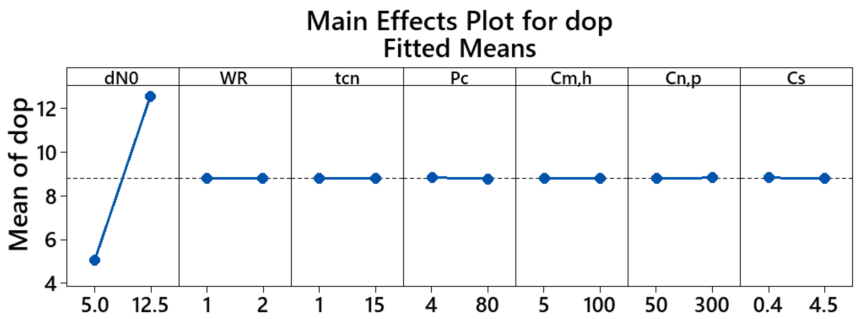
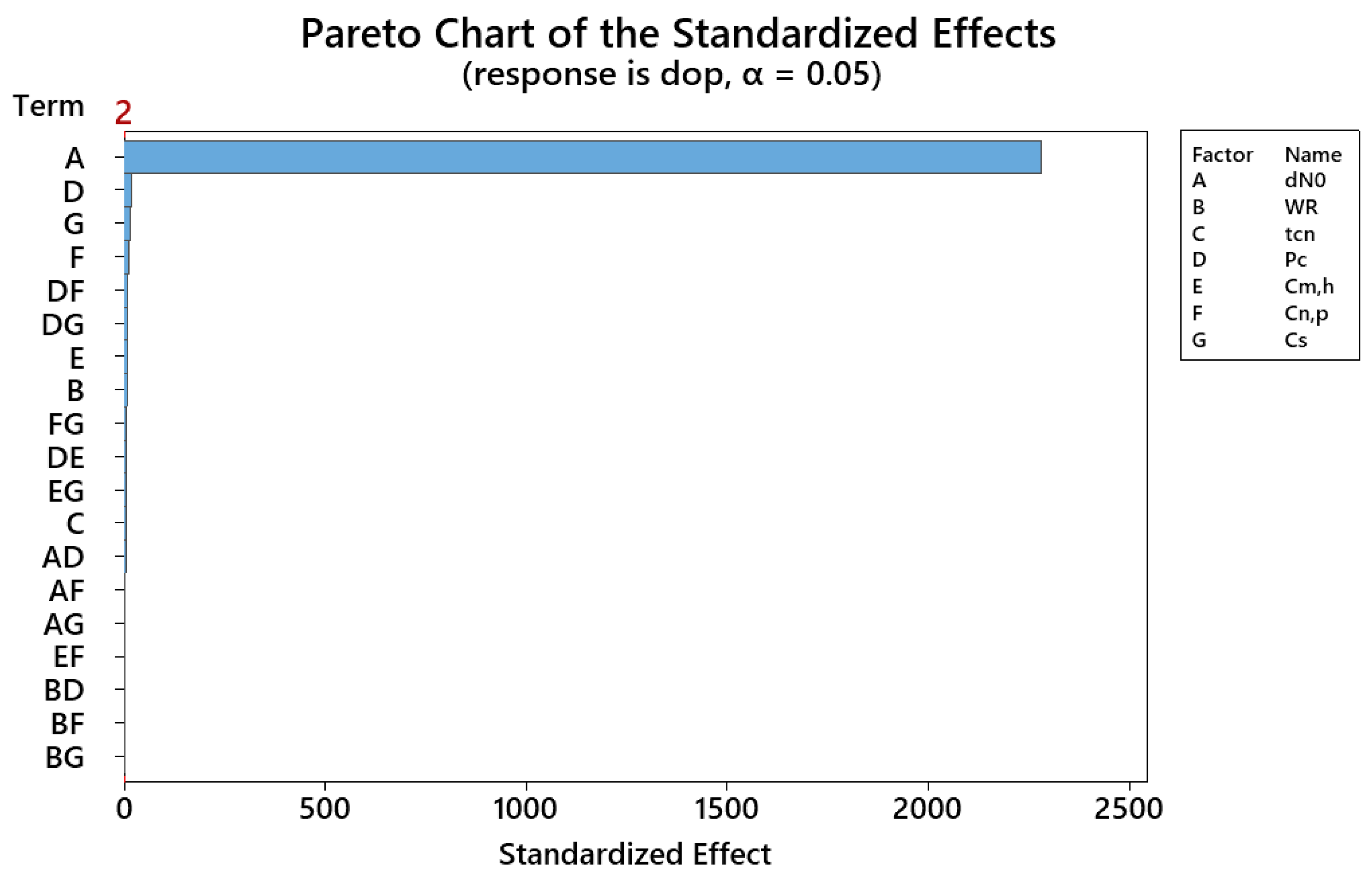
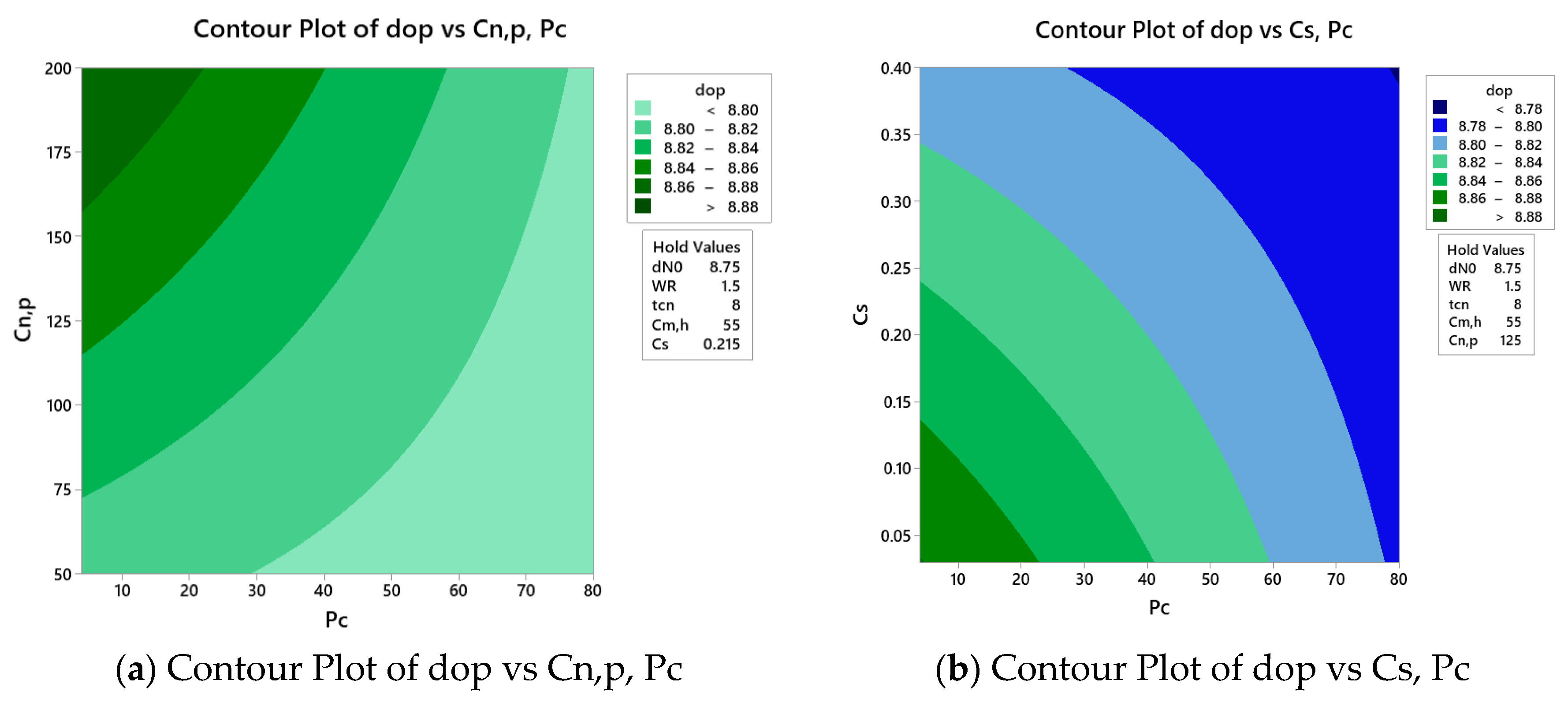
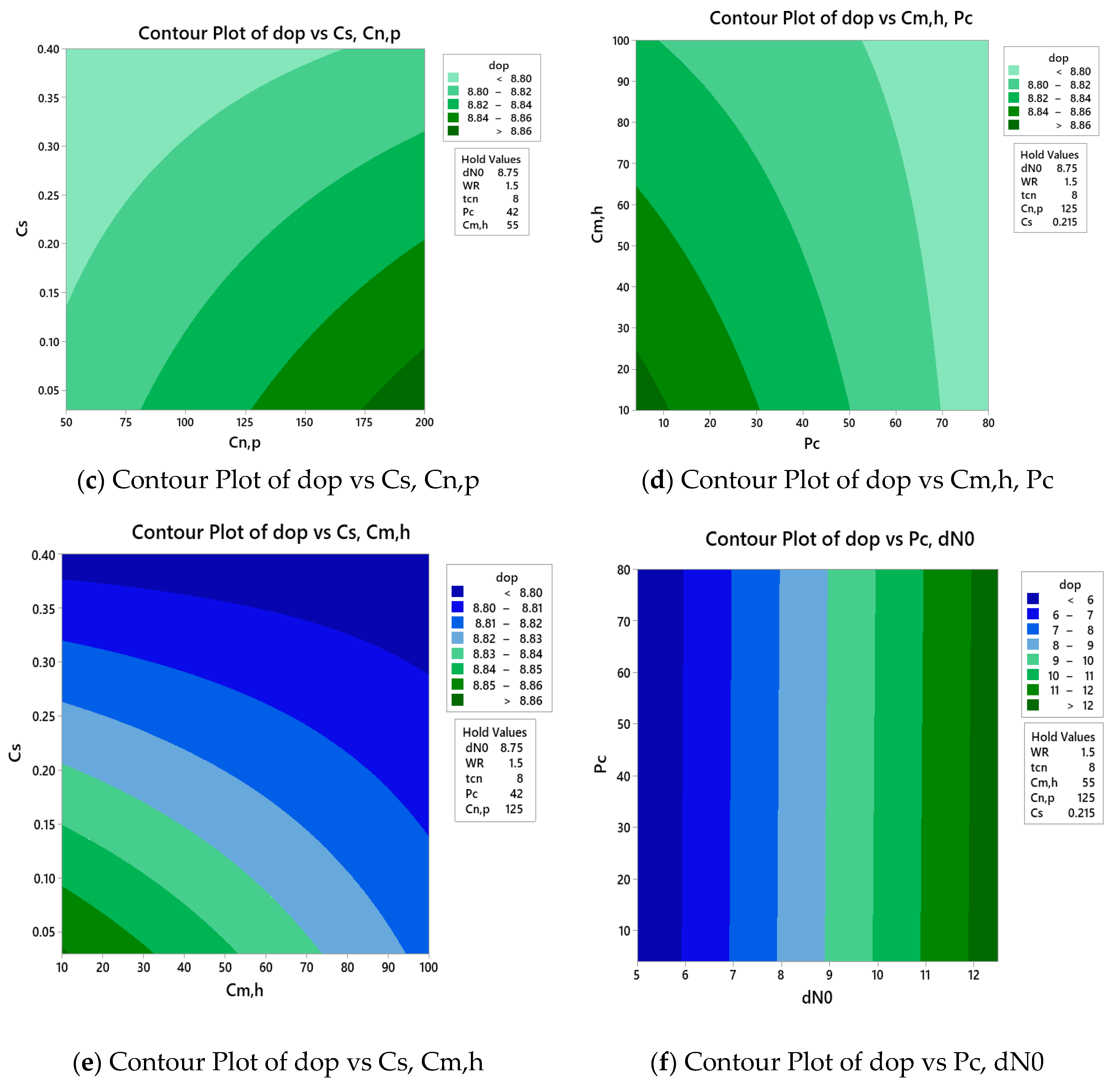
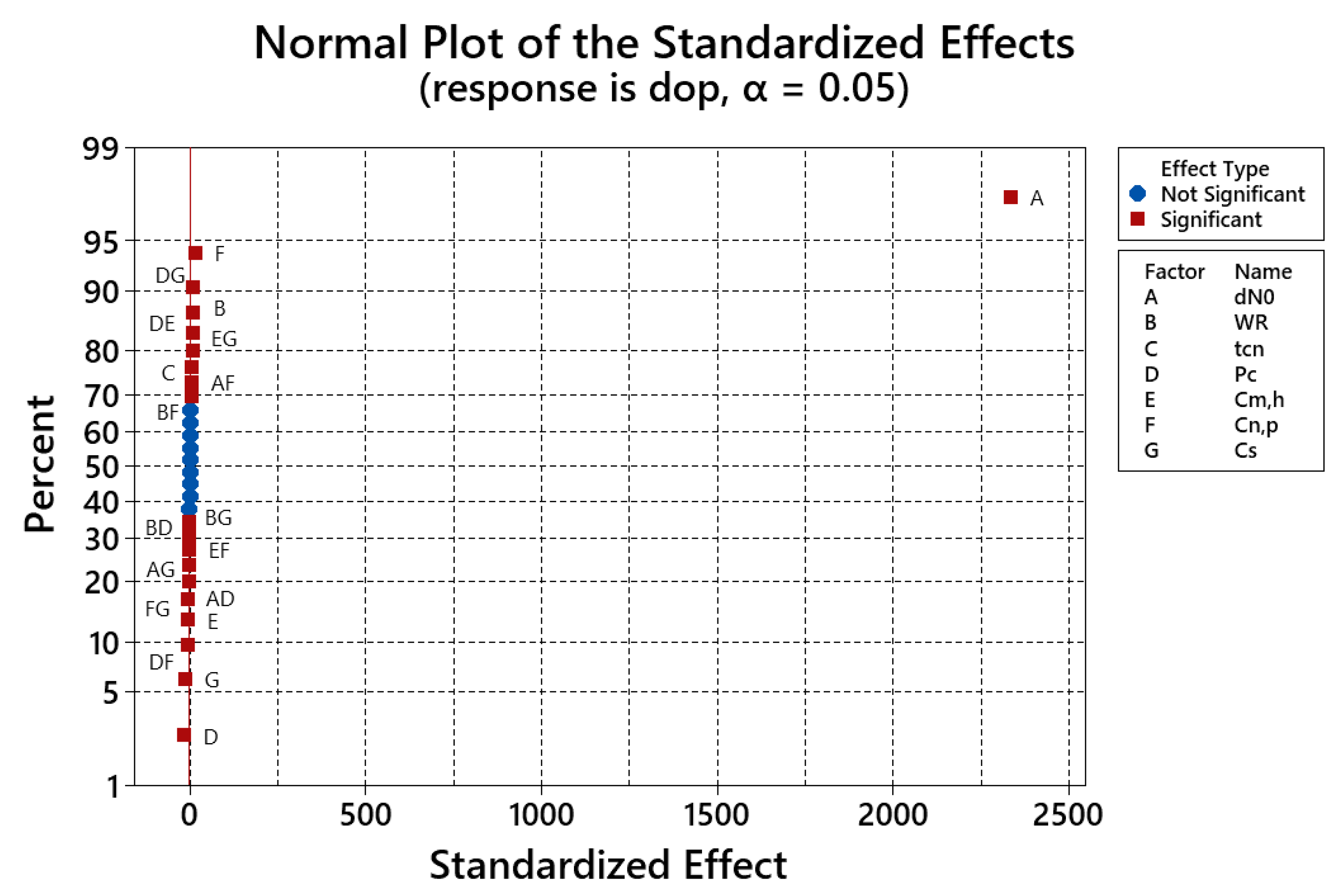
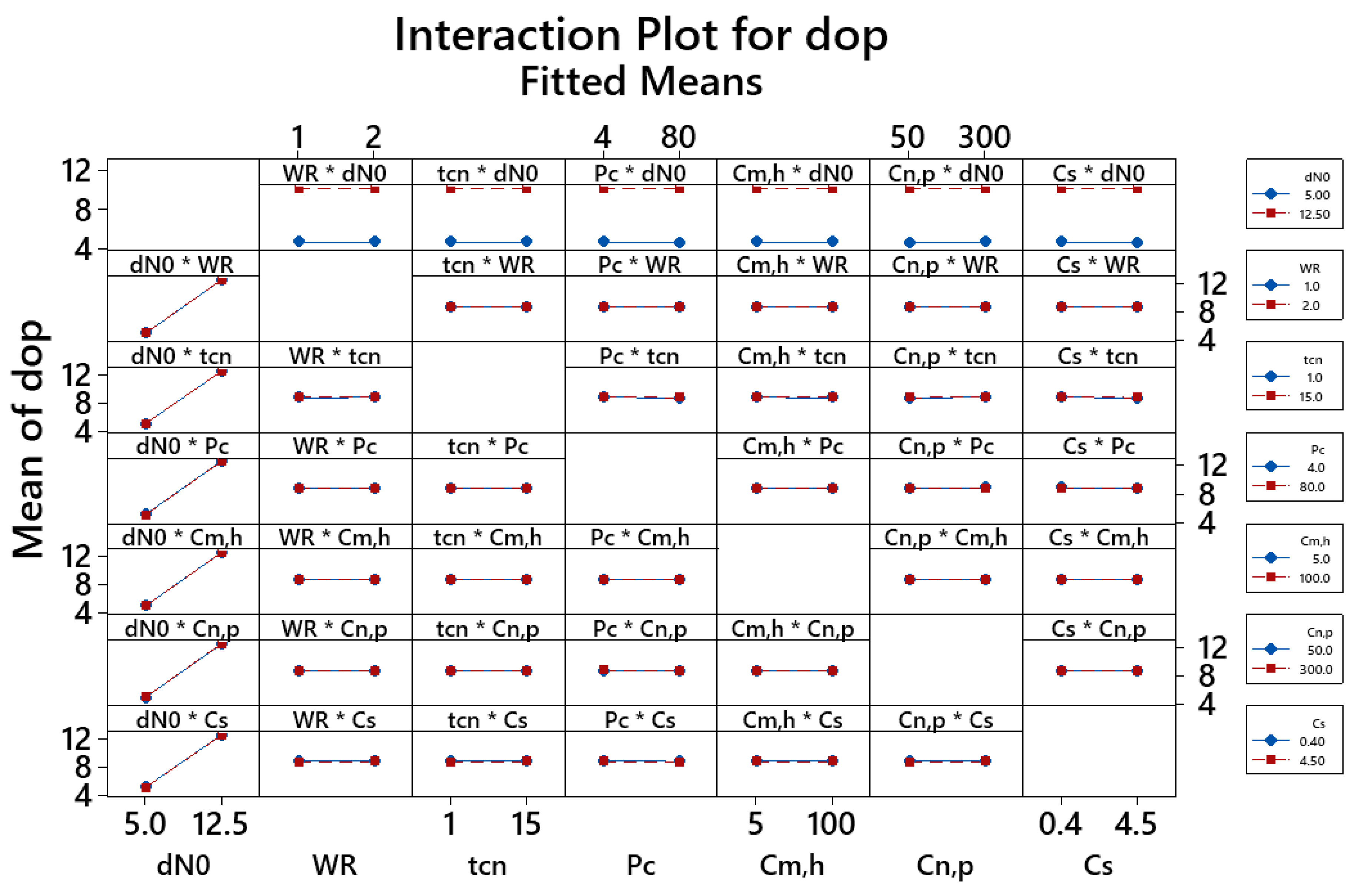
4.1. The Influence of Main Parameters and Their Interactions

The single influence of each input parameter on the response, the initial optimum diameter d_op, is graphically presented in Figure 6 (main effects plot). It is obvious that the initial nozzle diameter d_N0 has the strongest impact on the response, which is the positive impact, i.e., d_op increases with increase in d_N0 value from 5 to 12.5. Additionally, the parameters of ${\mathit{C}}_{\mathit{n},\mathit{p}}$ (F), $\mathit{W}\mathit{R}$ (B), and ${\mathit{t}}_{\mathit{c}\mathit{n}}$ (C) also have positive effects. On the contrary, ${\mathit{P}}_{\mathit{c}}$ (D), ${\mathit{C}}_{\mathit{s}}$ (G), and ${\mathit{C}}_{\mathit{m},\mathit{h}}$ (E) negatively impact the response. In terms of quantification, the influence of input parameters on the response are in the order of d_N0, ${\mathit{P}}_{\mathit{c}}$, ${\mathit{C}}_{\mathit{n},\mathit{p}}$, ${\mathit{C}}_{\mathit{s}}$, ${\mathit{C}}_{\mathit{m},\mathit{h}}$, $\mathit{W}\mathit{R}$, and ${\mathit{t}}_{\mathit{c}\mathit{n}}$. Nevertheless, it is difficult to distinguish these influences, hence a normal plot and a Pareto chart of the standardized effects can give more details about this.

The Pareto chart of the standardized effects is shown in Figure 7, where the influence of each single input parameter is orderly arranged. In this case, a given input parameter is considered as statistically significant to the response at the level of 0.05. Again, the dominant impact of the initial nozzle diameter on the optimum initial nozzle diameter is apparently noticed.

The influencing degree on the response progressively descends, as documented above: initial nozzle diameter (${\mathit{d}}_{\mathit{n}\mathbf{0}}$), compressor power (${\mathit{P}}_{\mathit{c}}$), nozzle cost per piece (${\mathit{C}}_{\mathit{n},\mathit{p}}$), cost of sand (${\mathit{C}}_{\mathit{s}}$), machine cost per hour (${\mathit{C}}_{\mathit{m},\mathit{h}}$), nozzle wear rate per hour ($\mathit{W}\mathit{R}$), and time for changing a nozzle (${\mathit{t}}_{\mathit{c}\mathit{n}}$). However, it is comprehended that the impact levels of the last six parameters are minor.

Only two parameters are counted as varying, while five remaining are constantly fixed. Regarding the evolution in Figure 8a in which five ranges of colors exhibit correspondingly five different values of the response. It is observed that when Pc increases, the response decreases, a positive influence. In case of Cn,p, an increase in Cn,p leads to increase in the response, corresponding to a negative impact. However, it is noticed that the increment value of the response between colors are minor. This means that the Cn,p and Fc factors have little influence on the response which is previously presented in Figure 6. The minor impacts of input parameters on the response can be similarly seen in Figure 8b–e. However, the influence of dN0 on the response is huge and can be profoundly observed in Figure 8f. In this situation the color ranges are bigger than previous ones and value corresponding to each range is higher also.

Another way to express the impact degree of the input parameters is to use a normal plot, which is distinctly depicted in Figure 9. We can easily see that, excepting for the influence of the initial nozzle diameter (${\mathit{d}}_{\mathit{n}\mathbf{0}}$), the effects of the remaining factors are almost identical when they are straightly placed. This tendency is also observed in the Pareto chart as mentioned above (cf. Figure 7). Moreover, it is noticed that the interactions between the separate parameters also have an influence on the optimum initial nozzle diameter (${\mathit{d}}_{\mathit{o}\mathit{p}}$). Indeed, the results in both Figure 6 and Figure 7 reveal that the combination between ${\mathit{P}}_{\mathit{c}}$ and ${\mathit{C}}_{\mathit{s}}$ (DG), ${\mathit{P}}_{\mathit{c}}$ and ${\mathit{C}}_{\mathit{m},\mathit{h}}$ (DE), ${\mathit{C}}_{\mathit{m},\mathit{h}}$ and ${\mathit{C}}_{\mathit{s}}$ (EG), and ${\mathit{d}}_{\mathit{n}\mathbf{0}}$ and ${\mathit{C}}_{\mathit{n},\mathit{p}}$ (AF) have positive impacts, while ${\mathit{P}}_{\mathit{c}}$ and ${\mathit{C}}_{\mathit{n},\mathit{p}}$ (DF), Cn,p and ${\mathit{C}}_{\mathit{s}}$ (FG), ${\mathit{d}}_{\mathit{n}\mathbf{0}}$ and ${\mathit{P}}_{\mathit{c}}$ (AD), ${\mathit{d}}_{\mathit{n}\mathbf{0}}$ and ${\mathit{C}}_{\mathit{s}}$ (AG), ${\mathit{C}}_{\mathit{m},\mathit{h}}$ and ${\mathit{C}}_{\mathit{n},\mathit{p}}$ (EF), $\mathit{W}\mathit{R}$ and ${\mathit{P}}_{\mathit{c}}$ (BD), and $\mathit{W}\mathit{R}$ and ${\mathit{C}}_{\mathit{s}}$ (BG) have negative effects on the response.

The interactions of the input parameters are deeply detailed in Figure 10 where it is easy to observe the most significant influence of the initial nozzle diameter when combined with others. When d_N0 varies from 5.0 to 12.5, its combination with other factors also increases. The similar behaviors are not obviously visualized in other cases. For instance, regarding the interaction between nozzle cost per piece (${\mathit{C}}_{\mathit{n},\mathit{p}}$) and cost of sand (${\mathit{C}}_{\mathit{s}}$) when ${\mathit{C}}_{\mathit{n},\mathit{p}}$ is changed from 50 to 300, the interaction (${\mathit{C}}_{\mathit{n},\mathit{p}}·{\mathit{C}}_{\mathit{s}}$) mostly stably varies.

4.2. The Proposed Regression Model of the Response

A proposed regression model with two interaction factors will be introduced via Minitab^@19 where the significance of the model is chosen as α = 0.05. The coefficients for the response are listed in

Table 3. Estimated effects and coefficients for d_op.

Term	Effect	Coef	SE Coef	T-Value	p-Value	VIF
Constant		8.81664	0.00165	5336.88	0.000
dN0	7.52984	3.76492	0.00165	2278.98	0.000	1.00
WR	0.02297	0.01148	0.00165	6.95	0.000	1.00
tcn	0.01578	0.00789	0.00165	4.78	0.000	1.00
Pc	−0.05641	−0.02820	0.00165	−17.07	0.000	1.00
Cm,h	−0.02359	−0.01180	0.00165	−7.14	0.000	1.00
Cn,p	0.04297	0.02148	0.00165	13.00	0.000	1.00
Cs	−0.04484	−0.02242	0.00165	−13.57	0.000	1.00
dN0 × Pc	−0.01359	−0.00680	0.00165	−4.11	0.000	1.00
dN0 × Cn,p	0.01078	0.00539	0.00165	3.26	0.001	1.00
dN0 × Cs	−0.01078	−0.00539	0.00165	−3.26	0.001	1.00
WR × Pc	−0.00984	−0.00492	0.00165	−2.98	0.004	1.00
WR × Cn,p	0.00766	0.00383	0.00165	2.32	0.022	1.00
WR × Cs	−0.00703	−0.00352	0.00165	−2.13	0.036	1.00
Pc × Cm,h	0.02172	0.01086	0.00165	6.57	0.000	1.00
Pc × Cn,p	−0.02797	−0.01398	0.00165	−8.47	0.000	1.00
Pc × Cs	0.02672	0.01336	0.00165	8.09	0.000	1.00
Cm,h × Cn,p	−0.01016	−0.00508	0.00165	−3.07	0.003	1.00
Cm,h × Cs	0.02016	0.01008	0.00165	6.10	0.000	1.00
Cn,p × Cs	−0.02203	−0.01102	0.00165	−6.67	0.000	1.00

. It should be noticed that in the model, the factors having no influence on the response are excluded. Oppositely, the factors which occur in the model are the ones with p-values inferior to the significance threshold (α = 0.05). For example, the interaction of $\mathit{W}\mathit{R}·{\mathit{C}}_{\mathit{s}}$ has a p-value of 0.036, which is smaller than 0.05. Hence, it can be concluded that this combination is statistically significant to the model. Moreover, it is realized that the minimum R-squared value is approximately 100%. This means that the experimental data are highly consistent with the developed model.

$$\begin{array}{cc}\hfill d_{op}=& -0.0022+1.00569 {\mathrm{d}}_{\mathrm{N}0}+0.03153 \mathrm{WR}+0.001127 {\mathrm{t}}_{\mathrm{cn}}-0.000157 {\mathrm{P}}_{\mathrm{c}}-0.000605 {\mathrm{C}}_{\mathrm{m},\mathrm{h}}+0.000253\hfill \\ \hfill & {\mathrm{C}}_{\mathrm{n},\mathrm{p}}-0.00477 {\mathrm{C}}_{\mathrm{s}}-0.000048 {\mathrm{d}}_{\mathrm{N}0}\times {\mathrm{P}}_{\mathrm{c}}+0.000011 {\mathrm{d}}_{\mathrm{N}0}\times {\mathrm{C}}_{\mathrm{n},\mathrm{p}}-0.000701 {\mathrm{d}}_{\mathrm{N}0}\times {\mathrm{C}}_{\mathrm{s}}-0.000259 \mathrm{WR}\times {\mathrm{P}}_{\mathrm{c}}\hfill \\ \hfill & +0.000061 \mathrm{WR}\times {\mathrm{C}}_{\mathrm{n},\mathrm{p}}-0.00343 \mathrm{WR}\times {\mathrm{C}}_{\mathrm{s}}+0.000006 {\mathrm{P}}_{\mathrm{c}}\times {\mathrm{C}}_{\mathrm{m},\mathrm{h}}-0.000003 {\mathrm{P}}_{\mathrm{c}}\times {\mathrm{C}}_{\mathrm{n},\mathrm{p}}+0.000171\hfill \\ \hfill & {\mathrm{P}}_{\mathrm{c}}\times {\mathrm{C}}_{\mathrm{s}}-0.000001 {\mathrm{C}}_{\mathrm{m},\mathrm{h}}\times {\mathrm{C}}_{\mathrm{n},\mathrm{p}}+0.000103 {\mathrm{C}}_{\mathrm{m},\mathrm{h}}\times {\mathrm{C}}_{\mathrm{s}}-0.000043 {\mathrm{C}}_{\mathrm{n},\mathrm{p}}\times {\mathrm{C}}_{\mathrm{s}}\hfill \end{array}$$

(10)

4.3. Analysis of Variance (ANOVA)

The analysis of variance is essential for the quantitative estimations of the impacting degree of each input parameter and their interactions on the response.

Table 4. Analysis of Variance.

Source	DF	Adj SS	Adj MS	F-Value	p-Value
Model	19	1814.74	95.51	273412.53	0.000
Linear	7	1814.62	259.23	742072.82	0.000
dN0	1	1814.35	1814.35	5193742.81	0.000
WR	1	0.02	0.02	48.33	0.000
tcn	1	0.01	0.01	22.81	0.000
Pc	1	0.10	0.10	291.45	0.000
Cm,h	1	0.02	0.02	50.99	0.000
Cn,p	1	0.06	0.06	169.13	0.000
Cs	1	0.06	0.06	184.21	0.000
2-Way Interactions	12	0.11	0.01	27.37	0.000
dN0 * Pc	1	0.01	0.01	16.93	0.000
dN0 * Cn,p	1	0.00	0.00	10.65	0.001
dN0 * Cs	1	0.00	0.00	10.65	0.001
WR * Pc	1	0.00	0.00	8.88	0.004
WR * Cn,p	1	0.00	0.00	5.37	0.022
WR * Cs	1	0.00	0.00	4.53	0.036
Pc * Cm,h	1	0.02	0.02	43.21	0.000
Pc * Cn,p	1	0.03	0.03	71.66	0.000
Pc * Cs	1	0.02	0.02	65.39	0.000
Cm,h * Cn,p	1	0.00	0.00	9.45	0.003
Cm,h * Cs	1	0.01	0.01	37.22	0.000
Cn,p * Cs	1	0.02	0.02	44.46	0.000
Error	108	0.04	0.00
Total	127	1814.77
Model Summary
S	R-sq	R-sq(adj)	R-sq(pred)
0.0186905	100.00%	100.00%	100.00%

shows the p-values of some parameters. It is seen that all parameters and some interactions also have statistical significance when their p-values are lower than 0.05, such as d_N0 (A), WR (B), t_nc (C), P_c (D), C_m,h (E), C_n,p (F), C_s (G), d_N0 * P_c (AD), d_N0 * C_n,p (AF), d_N0 * C_s (AG), WR * P_c (BD), WR * C_n,p (BF), WR * C_s (BG), P_c * C_n,p (DF), P * C_m,h (DE), P_c * C_s (DG), C_m,h * C_n,p (EF), C_m,h * C_s (EG), C_n,p * C_s (FG).

4.4. Validation of Proposed Model

In order to draw conclusions about the reliability of the model, the normal probability and observation order plots (cf. Figure 11) are necessarily considered. It is seen that the data shown in Figure 11a are almost the normal distribution. Moreover, the versus order plot (cf. Figure 11b) also reveals that the data are randomly distributed on the graph and not dependent on any controlling exception for the input parameters. Therefore, it can be concluded that the relationship between the optimum initial nozzle diameter, the response, and input parameters are crucially reliable.

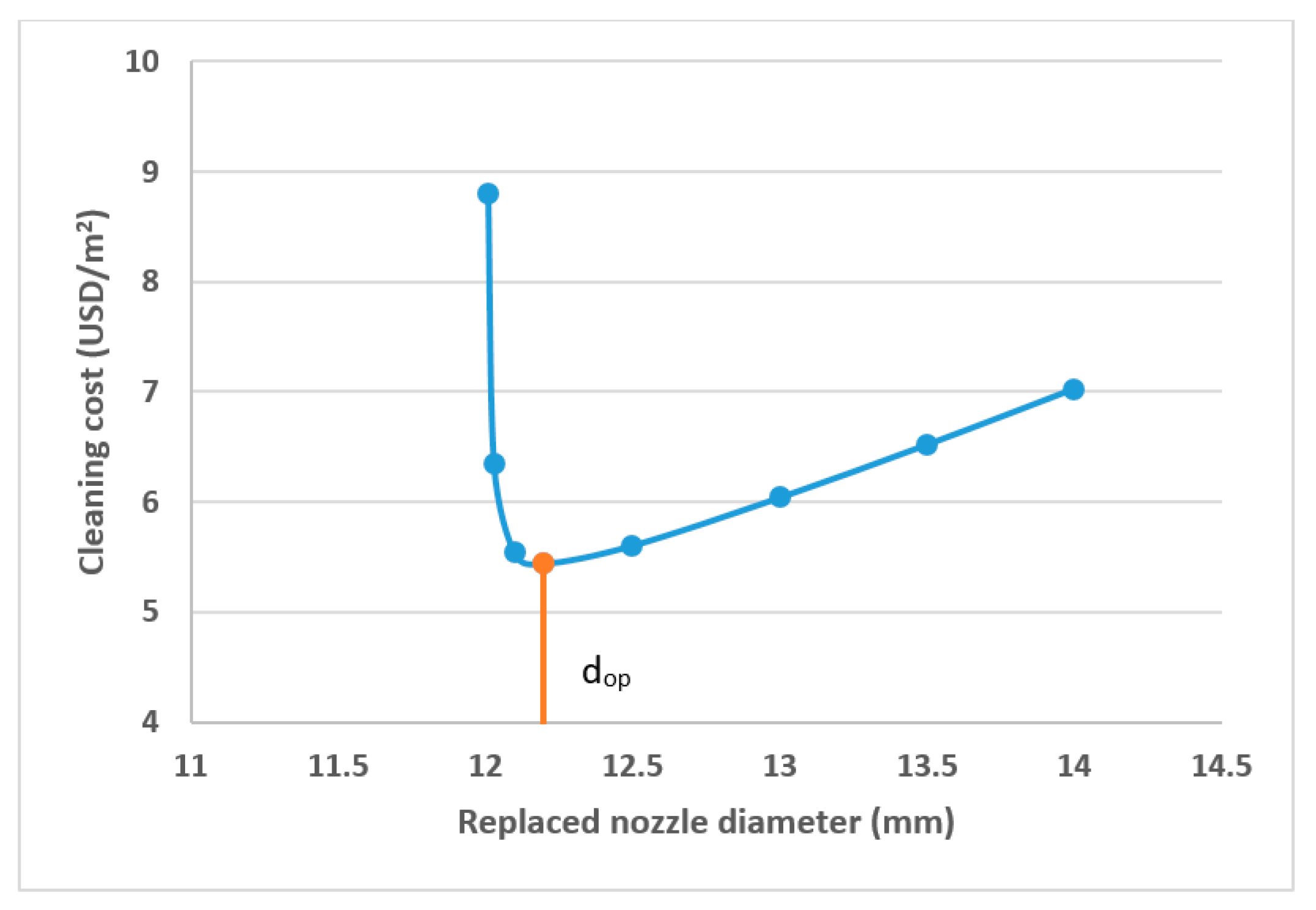
4.5. Benefits of Using Optimum Replaced Nozzle Diameter

To illustrate the benefit of using the optimum replaced nozzle diameter, the following example has been conducted. In this example, it is assumed that 1000 (m²) of metal surface needs to be cleaned by sand blasting. Also, the following input process parameters were chosen: $d_{N0}=6.5$ (mm); $WR=0.003$ (mm/h); $t_{cn}=15$ (min.); $P_c=30$ (kW); $C_{m,h}=20$ (USD/h); $C_{n,p}=200$ (USD/piece); $C_s=0.2$ (USD/kg). The calculated results in both traditional and optimum cases are presented in

Table 5. Example calculated results.

Parameter	Traditional Blasting	Optimum Blasting
Replaced nozzle diameter dN (mm)	8.09	7.0
Nozzle lifetime $L_n$ (h)	530	166.67
Average cleaning rate $v_{cl,a}$ (m2/h)	33.07	38.95
Total cleaning time (h)	30.24	25.67
Cleaning cost (USD/m2)	3.59	3.08
Total cleaning cost (USD)	3590	3080

. From the results, for cleaning 1000 (m²) of metal surface, the total time for cleaning was saved $30.24-25.67=4.57$ (h) and the total cleaning cost was reduced $3590-3080=510$ (USD). That means cleaning with optimum replaced nozzle diameter can save $\left(30.24-25.67\right)·100/30.24=15.11\%$ of the total cleaning time and $\left(30.24-25.67\right)·100/30.24=15.11\%$ of the total cleaning cost.

5. Conclusions

In this research work, a computer program was established to solve the objective function of optimizing the cost of blasting systems. The optimum initial nozzle diameter was constructed based on the objective function. The influences of the main design parameters (the input data) on the optimum initial nozzle diameter (d_op) of the blasting system have been investigated. Minitab^®19 was utilized for running the design of experiments. Based on the analyzed data, some conclusions should be made as follows.

✓

The initial nozzle diameter (d_N0) has the strongest impact on the optimum initial nozzle diameter (d_op), while the remaining input parameters have little effects.

✓

The interactions of some input parameters have important impacts on the optimum initial nozzle diameter.

✓

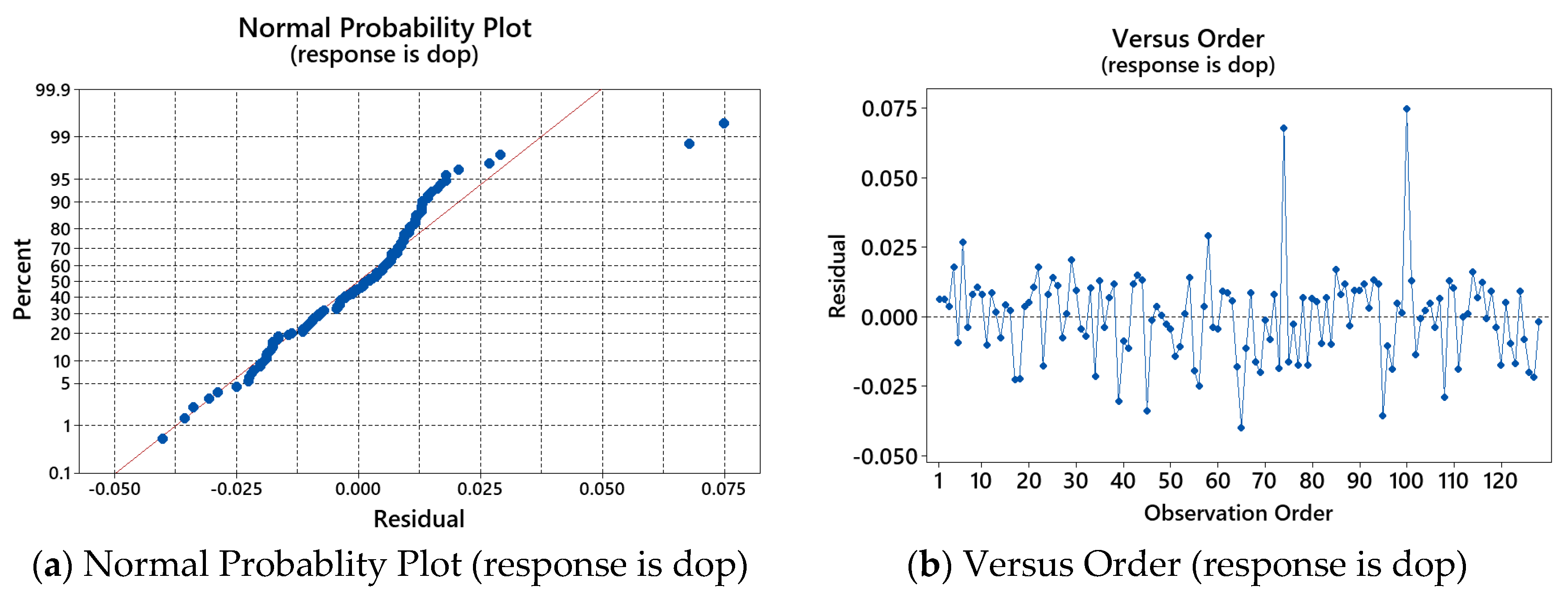
The factors of normal plots and versus observation plots show that the proposed regression model is mostly insistent to the experimental data, which are randomly distributed.

✓

The fitness between the data and the proposed model is reliable, which serves as an important base for deeper research. This can be used to calculate the optimum initial nozzle diameter of blasting systems to minimize the cleaning cost.

References

1. Kura, B.; Kambham, K.; Sangameswaran, S.; Potana, S. Atmospheric particulate emissions from dry abrasive blasting using coal slag. J. Air. Waste. Manag. Assoc. 2006, 56, 1205–1215. [Google Scholar] [CrossRef] [Green Version]
2. Global Abrasives Market Report. 2020. Available online: https://www.esherpamarketreports.com/reports/%EF%BB%BFglobal-abrasives-market-report-2020/ (accessed on 7 April 2020).
3. Pi, V.N.; Hoogstrate, A.M. Cost Optimization of Abrasive Blasting Systems: A New and Effective Way for Using Blasting Nozzles. Key Eng. Mater. 2007, 329, 323–328. [Google Scholar] [CrossRef]
4. Pi, V.N. Profit Optimization of Abrasive Blasting Systems. Key Eng. Mater. 2008, 389, 392–397. [Google Scholar] [CrossRef]
5. Pi, V.N.; Duc, T.M. A Study on Multi-Objective Optimization of Abrasive Blasting Systems. Adv. Mater. Res. 2010, 126, 29–34. [Google Scholar] [CrossRef]
6. Pi, V.N.; Chinh, P.C. A Study on Cost Optimization of Steel Shot Blasting Systems. Appl. Mech. Mater. 2011, 52, 568–572. [Google Scholar] [CrossRef]
7. Muthuramalingam, T. Effect of diluted dielectric medium on spark energy in green EDM process using TGRA approach. J. Clean. Prod. 2019, 238, 117894. [Google Scholar] [CrossRef]
8. Huo, J.; Liu, S.; Wang, Y.; Muthuramalingam, T.; Pi, V.N. Influence of process factors on surface measures on electrical discharge machined stainless steel using TOPSIS. Mater. Res. Express 2019, 6, 086507. [Google Scholar] [CrossRef]
9. Muthuramalingam, T. Measuring the influence of discharge energy on white layer thickness in electrical discharge machining process. Measurement 2019, 131, 694–700. [Google Scholar] [CrossRef]
10. Muthuramalingam, T.; Mohan, B. Enhancing the surface quality by iso pulse generator in EDM process. Adv. Mater. Res. 2013, 622, 380–384. [Google Scholar] [CrossRef]
11. Geethapriyan, T.; Kalaichelvan, K.; Muthuramalingam, T. Multi Performance Optimization of Electrochemical Micro-Machining Process Surface Related Parameters on Machining Inconel 718 using Taguchi-grey relational analysis. La Metall. Ital. 2016, 4, 13–19. [Google Scholar]
12. Geethapriyan, T.; Kalaichelvan, K.; Muthuramalingam, T. Influence of coated tool electrode on drilling Inconel alloy 718 in Electrochemical micro machining. Procedia CIRP 2016, 46, 127–130. [Google Scholar] [CrossRef] [Green Version]
13. Tung, L.A.; Hong, T.T.; Van Cuong, N.; Muthuramalingam, T.; Phan, N.H.; Hung, L.X.; Vu, N.P.A. Study on optimization of manufacturing time in external cylindrical grinding. In Proceedings of the International Conference on Engineering Research and Applications, Thai Nguyen, Vietnam, 1–2 December 2019; Springer: Cham, Switzerland, 2019; pp. 121–129. [Google Scholar]
14. Tran, T.H.; Luu, A.T.; Nguyen, Q.T.; Le, H.K.; Nguyen, A.T.; Hoang, T.D.; Vu, N.P. Optimization of Replaced Grinding Wheel Diameter for Surface Grinding Based on a Cost Analysis. Metals 2019, 9, 448. [Google Scholar] [CrossRef] [Green Version]
15. Tran, T.H.; Le, X.H.; Nguyen, Q.T.; Le, H.K.; Hoang, T.D.; Luu, A.T.; Vu, N.P. Optimization of replaced grinding wheel diameter for minimum grinding cost in internal grinding. Appl. Sci. 2019, 9, 1363. [Google Scholar] [CrossRef] [Green Version]
16. Ramamurthy, A.; Sivaramakrishnan, R.; Muthuramalingam, T. Taguchi-Grey Computation Methodology for Optimum Multiple Performance Measures on machining Titanium alloy in WEDM Process. Indian J. Eng. Mater. Sci. 2015, 22, 181–186. [Google Scholar]
17. Muthuramalingam, T.; Ramamurthy, A.; Sridharan, K.; Ashwin, S. Analysis of surface performance measures on WEDM processed titanium alloy with coated electrodes. Mater. Res. Express 2018, 5, 126503. [Google Scholar] [CrossRef]
18. Norton Sand Blasting Equipment, Nozzle Selection Guide and Information. Available online: http://www.nortonsandblasting.com/nsbnozzles2.html (accessed on 7 April 2020).
19. Abrasive Blast Nozzles. Available online: https://www.surfacefinishingcompany.com/wp-content/uploads/2009/10/Kennametal-Abrasive-Flow-Products-Catalog.pdf (accessed on 8 April 2020).
Figure 1. The shape of a nozzle diameter [19].
Applsci 10 03920 g001
Figure 2. Air pressure versus nozzle diameter.
Applsci 10 03920 g002
Figure 3. Cleaning rate versus replaced nozzle diameter.
Applsci 10 03920 g003
Figure 4. Relation between cleaning cost components and replaced nozzle diameter.
Applsci 10 03920 g004
Figure 5. Cleaning cost versus replaced nozzle diameter.
Applsci 10 03920 g005
Figure 6. Main effects plot for optimum initial nozzle diameter.
Applsci 10 03920 g006
Figure 7. Pareto chart of the standardized effects.
Applsci 10 03920 g007
Figure 8. Contour plots showing the evolution of the response vs input parameters.
Applsci 10 03920 g008aApplsci 10 03920 g008b
Figure 9. Normal plot for dop.
Applsci 10 03920 g009
Figure 10. The interactions between input parameters.
Applsci 10 03920 g010
Figure 11. Normal probability and versus order plot for dop.
Applsci 10 03920 g011