Acoustic Emission Monitoring of the Turin Cathedral Bell Tower: Foreshock and Aftershock Discrimination

1
Department of Structural, Geotechnical and Building Engineering, Politecnico di Torino – Corso Duca degli Abruzzi, 24, 10129 Torino, Italy
2
Masera Engineering Group s.r.l, 10129 Torino, Italy
*
Author to whom correspondence should be addressed.
Appl. Sci. 2020, 10(11), 3931; https://doi.org/10.3390/app10113931
Submission received: 10 March 2020
/
Revised: 11 May 2020
/
Accepted: 18 May 2020
/
Published: 5 June 2020
(This article belongs to the Special Issue Nondestructive Testing (NDT): Volume II)
Abstract
:Featured Application
The Acoustic Emission (AE) technique can be used to perform structural monitoring of historical buildings including tall masonry towers. In addition, the AE data detected on the structure, during the earthquake activity, can be used to discriminate foreshock and aftershock intervals.
Abstract
Historical churches, tall ancient masonry buildings, and bell towers are structures subjected to high risks due to their age, elevation, and small base-area-to-height ratio. In this paper, the results of an innovative monitoring technique for structural integrity assessment applied to a historical bell tower are reported. The emblematic case study of the monitoring of the Turin Cathedral bell tower (northwest Italy) is herein presented. First of all, the damage evolution in a portion of the structure localized in the lower levels of the tall masonry building is described by the evaluation of the cumulative number of acoustic emissions (AEs) and by different parameters able to predict the time dependence of the damage development, in addition to the 3D localization of the AE sources. The b-value analysis shows a decreasing trend down to values compatible with the growth of localized micro and macro-cracks in the portion of the structure close to the base of the tower. These results seem to be in good agreement with the static and dynamic analysis performed numerically by an accurate FEM (finite element model). Similar results were also obtained during the application of the AE monitoring to the wooden frame sustaining the bells in the tower cell. Finally, a statistical analysis based on the average values of the b-value are carried out at the scale of the monument and at the seismic regional scale. In particular, according to recent studies, a comparison between the b-value obtained by AE signal analysis and the regional activity is proposed in order to correlate the AE detected on the structure to the seismic activity, discriminating foreshock, and aftershock intervals in the analyzed time series.
1. Introduction
Historical buildings frequently show diffused crack patterns due to different problems (thermal loading, static and dynamic loadings, subsidence conditions, fatigue, and creep). Non-destructive methods allow us to evaluate the state of conservation of these structures and its time evolution [1,2,3,4,5]. During the last few years, the authors have conducted many studies through the application of a control method based on the spontaneous emission of elastic waves—the acoustic emission (AE) technique [6,7,8,9,10]. By AE monitoring, the signals, emitted by defects, are acquired by wide-band piezoelectric (PZT) sensors and successively post processed by statistical and analytical analysis. The AE technique is ideally suited for use in the assessment of historic and monumental structures that are subjected to different loading conditions [9,10]. Using the AE technique, the authors acquired considerable experience in the monitoring of historical buildings, such as tall masonry towers and monuments in which the bearing walls are made of stones, masonry systems, and sack masonry [6,7,9]. At first, different studies have been conducted on the structural stability of the medieval towers in Alba, a characteristic town in Piedmont (northwest Italy) [6,7]. Successively, the AE technique was employed for the controlling of the evolution of structural damage caused by repetitive phenomena (vehicle traffic loading, wind effects) such as in the case of the Asinelli Tower in Bologna (Central Italy) [6,10]. In the present study, the AE technique is used to determine the damage level in the bell tower of the Turin Cathedral for different monitoring periods during the restoration work of the facades and the top baroque cell containing the bells.
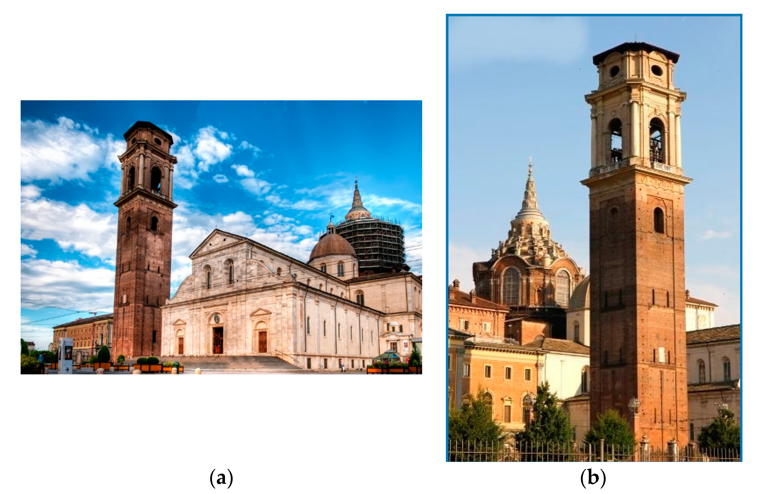
The bell tower was initially built in the second half of the 15th century between 1468 and 1470 [11,12]. Recently restored, the tower is inserted, today, in the Diocesan Museum of the Sabaudian city (see Figure 1). The masonry tower was erected completely by the will of bishop Giovanni di Compey (Figure 1a). Between 1720 and 1722, the court architect Filippo Juvarra worked on the crowning and the dome, the tower assumed its current appearance—a brick construction that ends with a baroque bell tower made by stone decorations [11,12] (see Figure 1b and Figure 2).
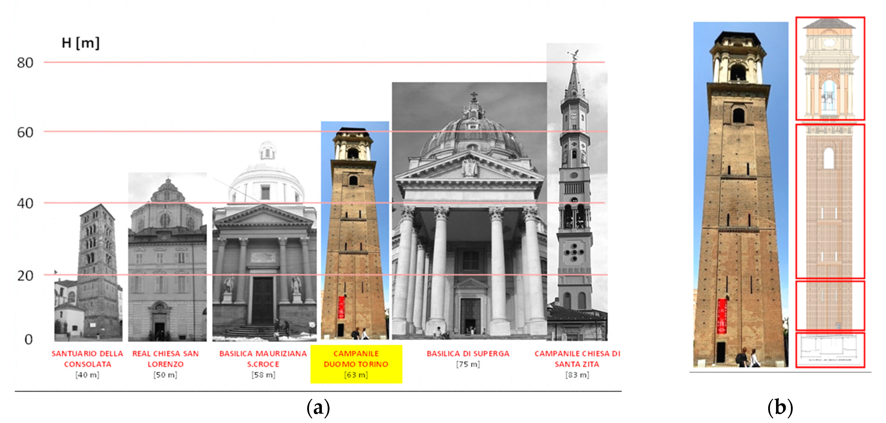
The bell tower is today the third tallest masonry building in the City, (63 m) (see Figure 2a). As mentioned, the structure, finished around 1470, was built next to the paleochristian complex of the so-called three churches, the communicating buildings of San Salvatore, Santa Maria, and San Giovanni Battista. Successively, the structure was incorporated into the building of San Giovanni. About 20 years later, the churches were destroyed, and in their place, the city’s cathedral was built. The brilliant architect Meo del Caprina designed the cathedral, and the original tower became the bell tower, connected to the church by an underground gallery that is now part of the Diocesan Museum (Figure 1a). The tower was restored for the first time in 1620, and a century after, the design of Filippo Juvarra was completed for the top cell and the roof. When the Palazzo Vecchio was demolished in the 19th century, the bell tower remained isolated and ignored until 1986, when contemporary restorations were started by the architects Maurizio and Giuseppe Momo. The tower, therefore, consists of two distinct parts: the 15th-century tower, with a squared plan erected on the site of the early Christian churches, still marked at the top by the opening of the ancient bell cell; and the 18th-century crowning—the unfinished realization of Filippo Juvarra’s project (Figure 2b). The ancient part is a square plan of about 10 meters (9.70 × 9.70) on each side with perimeter walls of a constant thickness (2 m) up to the Juvarrian crown, where, in correspondence to the bell cell, the square is connected to an octagon. The restorations of the 1980s were followed up in 2013 by the architects Maurizio and Chiara Momo. In the last few years, the bell tower was subjected to the last external restoration works that completely returned the tower to the city in all its magnificence (Figure 1b).
In the present study, a six-channel AE data acquisition system was used to evaluate the time evolution of the crack pattern in the masonry of the ancient bell tower. The investigation has been carried out using several statistical analyses and parameters for the assessment of the damage level reached in the monitored structure [13,14,15,16,17,18]. The AE sensors were positioned at the base of the tower between the first and the third level of the scaffolds (Figure 2b). The localization procedure, originally employed by the triangulation procedure, was successively refined by the authors using an improved version of the Akaike method, which is able to determine a reliable onset time determination of the AE signal acquisition time [19,20]. In addition, the statistical analysis based on the b-value determination were used in order to define the damage evolution in the masonry structures of the monument and the timber structure sustaining the bells inside the top cell.
In addition, the AE signal analysis was correlated to the seismic activity recorded in the region surrounding the monitoring site. A radius of 100 km was considered in order to evaluate the seismic region where the earthquake time series were collected from the Italian National Institute of Geology and Volcanology (I.N.G.V. http://terremoti.ingv.it/instruments). Furthermore, according to recent studies proposed by Guglia and Weimer [21], a real-time determination of aftershock and foreshock in the seismic times series is observed in the seismic time series near Turin for reduced magnitude levels. Finally, an original application of the procedure adopted for the seismic time series was also applied to the AE data, thus obtaining an impressive correlation to the earthquake activity. This evidence contributed significantly to the AE monitoring of tall building. not only for structural monitoring but also as a valid instrument for the determination (foreshock/aftershock) of regional seismicity.
2. Numerical Model of the Bell Tower
In the preliminary phase, the geometric relief preceded the numerical model of the structure; the survey of the bell tower was carried out with a laser-scanner tool that allows us to obtain the whole 3D geometry and every small detail of the building, totally defining the geometry, both internally and externally.
Starting from the results of the survey, FEM was implemented with the aid of Midas FX software (CSP Fea Engineering, Padova, Italy), a three-dimensional geometric modeler completed by the FEM modulus. Through the CAD (computer-aided drafting) reproduction, the geometric model of the tower was initially defined, from which, thanks to the software’s auto-meshing function, the FEM model was obtained. In Figure 3, the model obtained is shown.
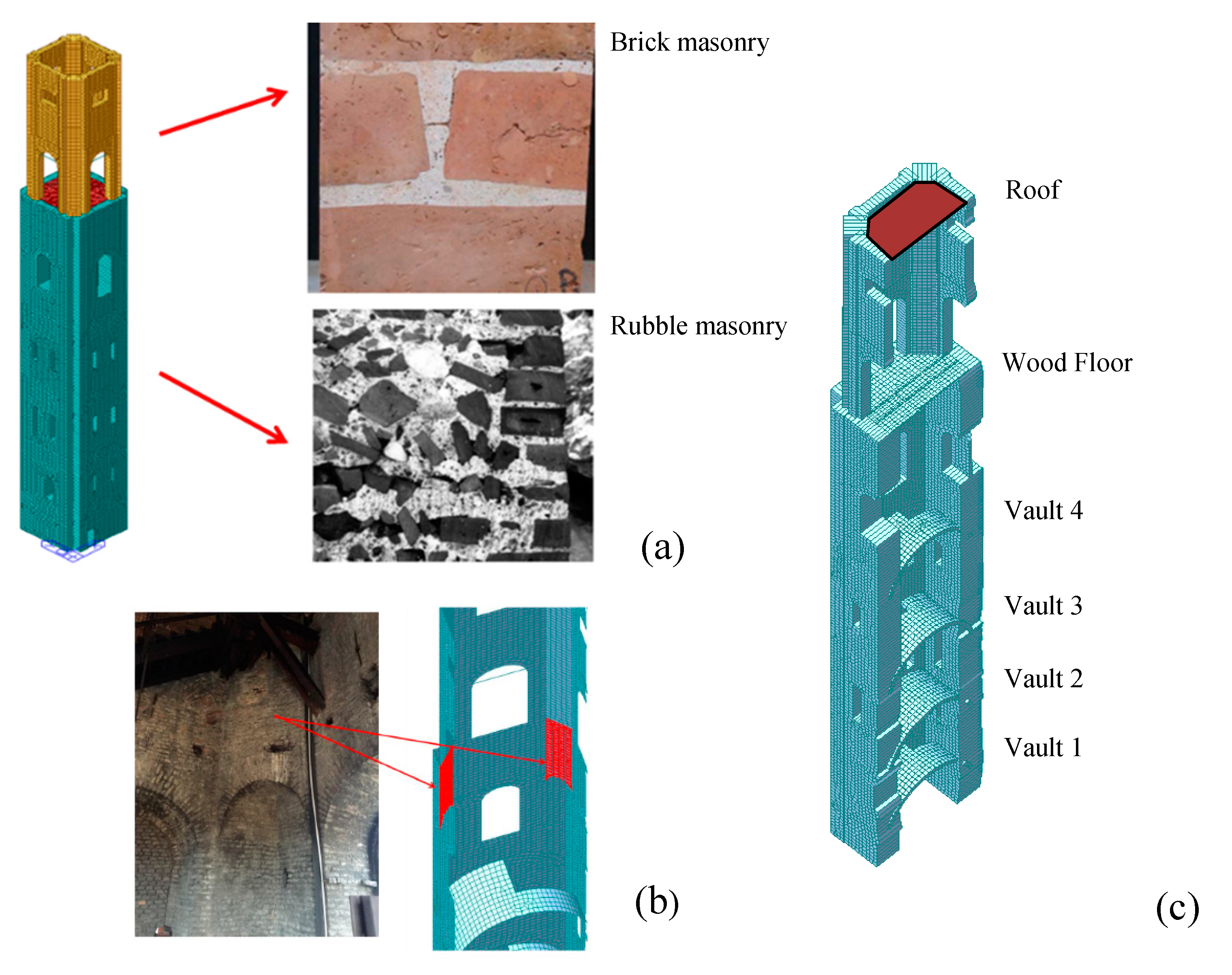
The geometric mesh is made up of 20.954 knots and 21.143 elements, 29 being of the “Truss” type, 162 of the “beam” type, and 20.952 of the ‘plate’ type. In the model, in addition to the external support walls, the floor elements and the vaulted ceilings were also modelled with flat 3D shell-like elements. Particular attention was paid to the modelling of the connection between the more ancient part of the tower (lower part) and the bell cell designed by the architect F. Juvarra, made with different materials and different shapes, as reported in Figure 3a. In Table 1, the properties of the materials employed during the simulations were reported. The materials used in the different parts of the model are clearly represented in Figure 1a,b for each levels of the tower. In particular, the rubble masonry (sack masonry) is the most used masonry type in the monument. This kind of building method is characterized by a rough, unhewn building stone set in mortar but not laid in regular courses. It may appear as the outer surface of a wall or may fill the core of a wall, which is faced with unit masonry such as ashlar or brick. This is the case of the Turin’s bell tower up to the roof level (about 40 m from the ground)-the part corresponding to the stem. On the other hand, the last level of the tower is characterized by brick masonry from the 18th century, corresponding to the proper bell cell (Table 1, Figure 1b and Figure 2b). The compressive stress (fm) of the rubble masonry was assumed to be the middle of that used for brick masonry. A similar ratio was assumed for the shear stress τ0, the elastic modulus E, and the shear modulus G. For the specific weight (γ), the values are almost the same for the two types of masonry (Table 1).
In addition, thin elements have been inserted (chain) (see Figure 3b), which act as connections between the two different parts of the tower-the stem and the cell. In this way, the loads of the bell cell are gradually transferred on the fifteenth-century part of the tower. Chains have also been inserted in the model in correspondence with the “key heads” observable from the outside; the external ‘keys’ and the inserted chains can be seen in Figure 3b. It can be observed that some chains do not circumscribe the tower; this is due to the fact that they have only been inserted in correspondence with the externally visible “keys.” This operation is therefore in favor of safety, since the chains are certainly less in number than those actually present in the structure.
Once the model was completed, it was subjected to a global static analysis, in which the loads were combined according to the fundamental combination (usually used for checks at the ultimate limit state (SLU)) and according to that characteristic or rare (usually used for checks on the limit state of exercise (SLE)), and on a linear dynamic analysis or a modal analysis. The first step consists in the evaluation of the confidence factor (Fc) for the reduction of the average resistance of the materials; this was calculated using the Italian circular no. 26 of December 2, 2010. The calculation of the (Fc) is reported in the following equation:
The difference in the materials as well as the presence of the four intermediate vaults, the intermediate, and the top roof were taken into consideration. In order to conduct the analysis, it was necessary to analyze in detail all the loads to which the structure is actually subjected. Among the vertical loads, we considered the permanent loads and the variable loads (related to the four vaults); the wooden floor and the top roof were also considered (see Table 2).
Finally, the weight of the four bells located in the bell cell was also considered (Table 3).
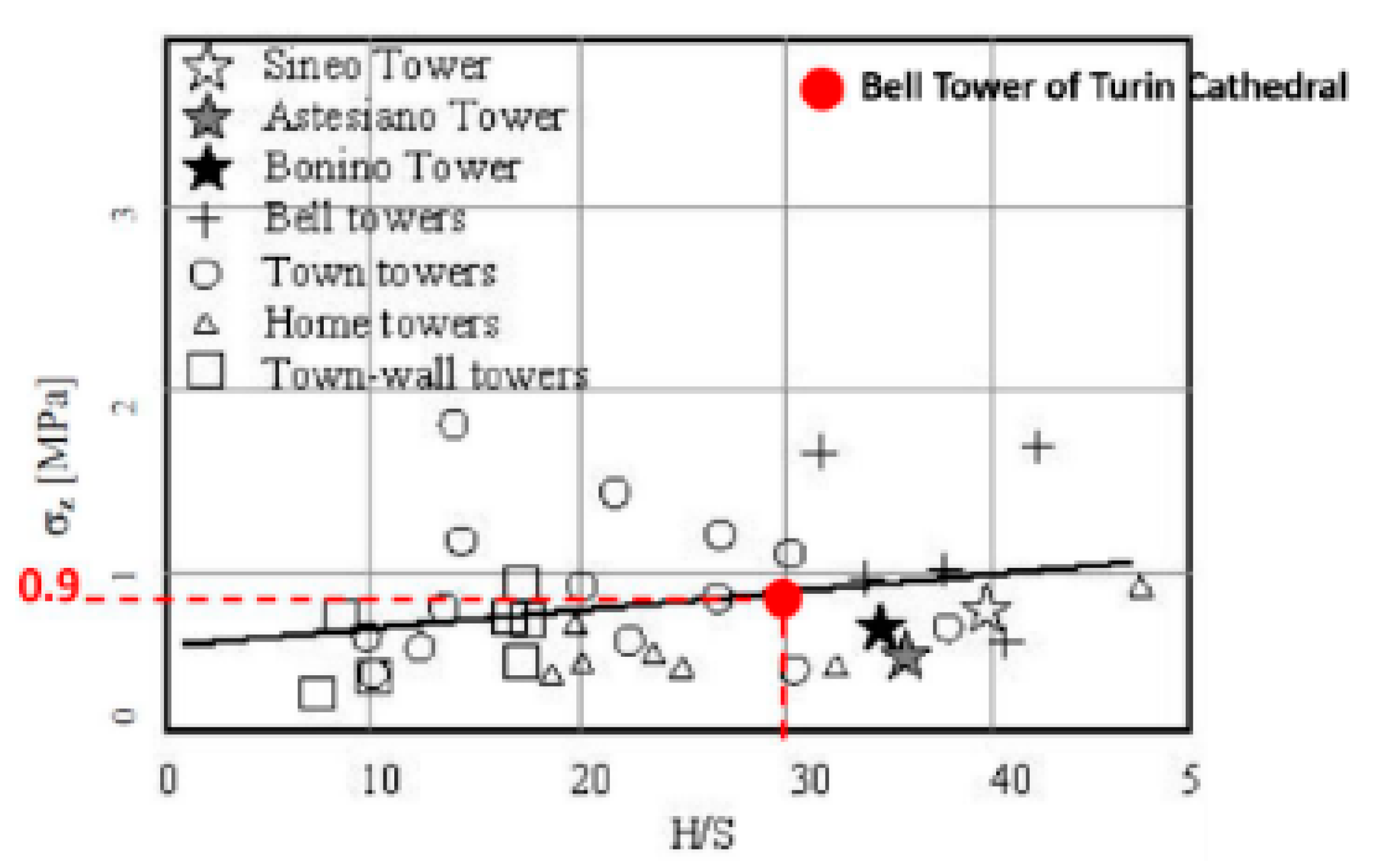
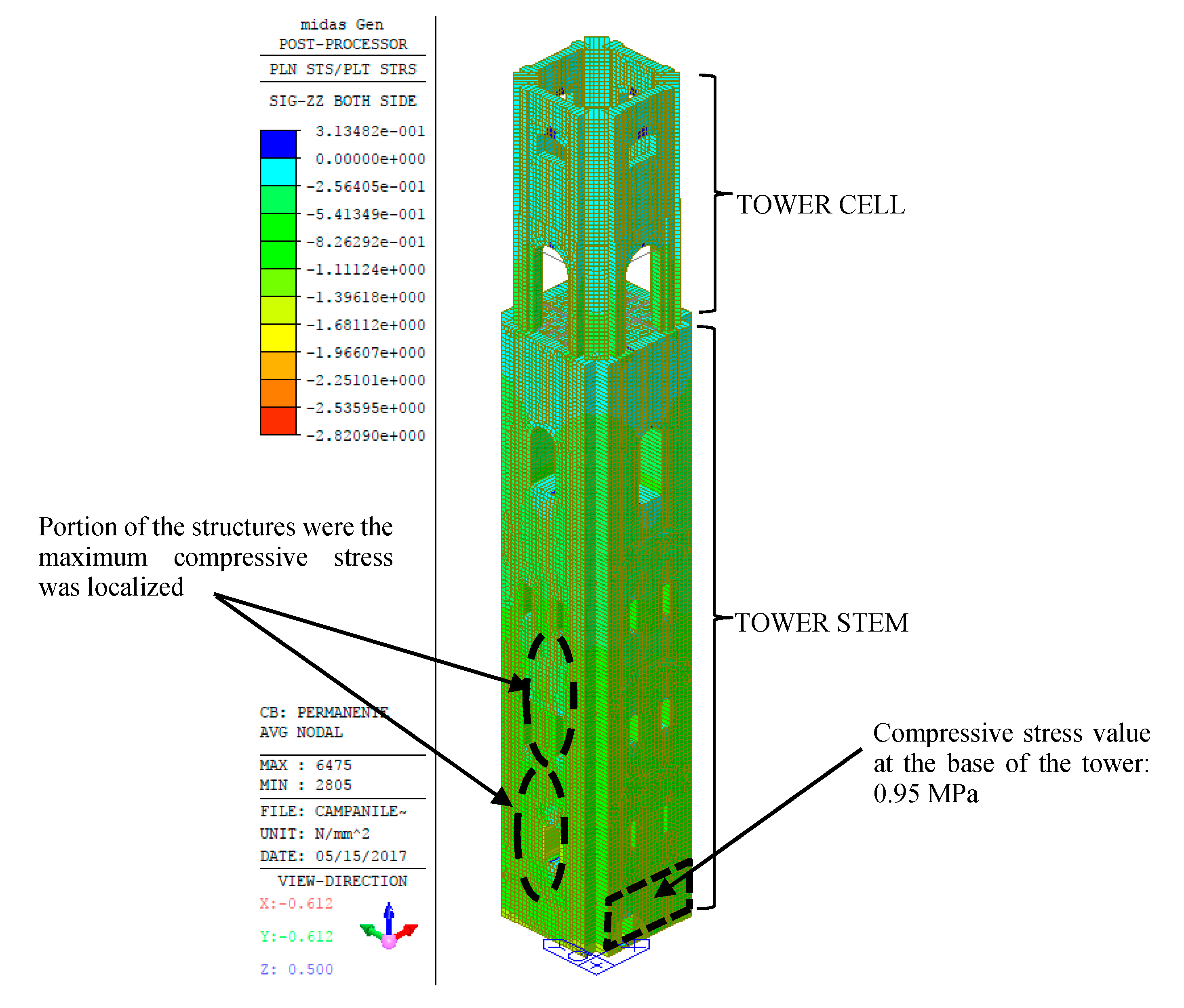
As far as the horizontal actions are concerned, the values of the seismic action and the pressure exerted by the wind on the tower were evaluated and implanted in the model. The weights of the various elements were assessed by multiplying their thickness by the specific weight of the materials, and in the case of the masonry vaults, taking into account a thickness equal to 30 cm and the specific weight equal to 18 kN/m3, a dead load of 5.0 daN in assumed. For the timber floor a thickness equal to 12 cm and a specific weight equal to 5.75 kN/mc is considered (Figure 3c,d). The vaults were considered susceptible to crowding, and therefore, an accidental load of 5 kN/m2 is assumed. As for the roof and the facades, snow, wind, and seismic loads were considered according to the Italian rules for the evaluation of these kind of actions. Figure 4 shows a detail of the area where the highest vertical tension values were found; the value at the base of the tower stress value obtained is about 0.95 MPa. In addition, the calculation of the compression stress at the base of the tower can be carried out with a rough approximation: σ = N/A= 66526/63.15 = 1.05 MPa. The stress value at the base of the tower obtained from the FEM model was compared with the results obtained [5,6,7,8,9,10] for different masonry towers and tall buildings. In particular, the values obtained for the tower are similar to that showed in the trend of vertical tensions as the reported heights of the towers [9].
In term of comparison to the real scenario, and in order to validate the results of the implemented model, the value of the maximum compressive stress obtained by the simulations at the base of the tower was compared to the values reported in the literature for similar Italian ancient masonry towers, characterized by similar base vs. height ratio, constructive techniques and elastic properties of the constituting materials [22]. In particular, in Figure 4, the stress value obtained at the base of the tower by the simulations (0.95 MPa) were put in the graph where the compressive stress at ground level of similar monuments were reported. The value obtained are perfectly in agreement with the others and can be considered well validated.
The results of the static analysis are reported in Figure 5. The value of the compressive stress, as reported previously, was equal to 0.95 MPa at the base of the tower. On the other hand, in a localized portion of the structure, related to the opening disposition, the compressive stress reached higher values up to 1.4 MPa. These values were observed particularly on the south façade of the tower, between the second and the third level.
This evidence, together with the evaluation of the cracking pattern, were useful for the definition of the AE device application. The analyses carried out by the model proved particularly useful for the realization of the AE monitoring. The previous realization of numerical models helps us to correctly understand where the AE sensors must be focused. As reported in recent works [6,7,8,9,10], the AE monitoring cannot take under a control of a very large extension in term of the volume of the structure constituting the monitored building, especially in the case where the structure was built from sack and rubble masonry. The AE signal transmission, in fact, is connected to the degree of disorder of the propagating medium—the greater the level of the disorder, the higher the amount of the reflected/refracted part of the signal [9]. In agreement with this evidence, the numerical model was fundamental in circumscribing the area of the structure where the AE monitoring should be applied. In particular, the highest stress levels found in the model were localized at the base of the tower between the second and third levels, allowing us to select this part and also the correspondent side of the building as the most suitable places for the AE analysis.
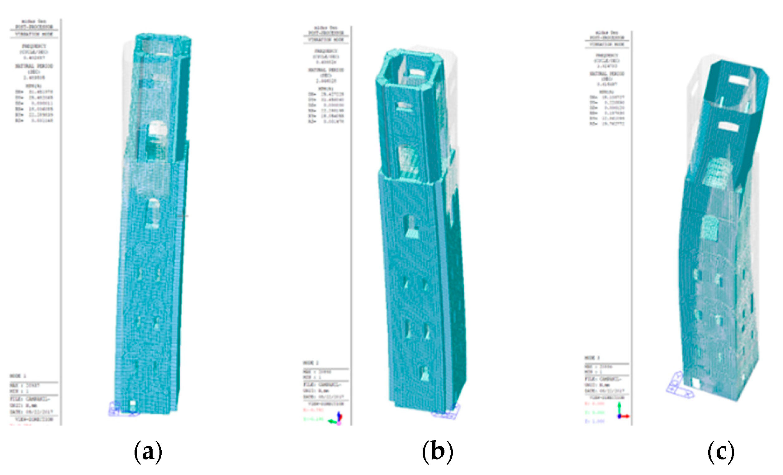
In order to further validate the numerical model, the results of the modal analysis are shown in Figure 6, and the first three vibrating modes were investigated and reported. It can be observed that the first and second modes are flexional, characterized mainly by displacements in x and y directions, while the third is torsional. In Table 4 and Table 5, the results of eigenvalue analysis and the masses participating in the individual modes were reported. In the last table, the values of the predominant masses of the first three vibrating modes have been highlighted. The period T related to the first vibrating mode was also calculated analytically and reported in the following Equation:
In Equation (2), H is the height of the tower, ρ is the radius of inertia, γ is the specific weight of the masonry (expressed in kg/m3), E is the elastic modulus of the masonry, and g is the gravitational acceleration.
3. Materials and Methods
The increased necessity for continuous survey of infrastructures, ancient buildings, and monuments requires wireless transmission and processing of large amounts of data, thus allowing remote and real-time monitoring to point out the presence of evolving structural damage processes. To this purpose, the cooperation between the AE research unit of the Politecnico di Torino and the Italian company Lunitek SRL (Sarzana-Italy) produced the AEmission® system for structural and seismic monitoring, based on AE data acquisition and transmission [23]. An array of eight piezoelectric (PZT) transducers is connected to this multi-channel system (each channel with a devoted memory of 64 Mb), which automatically stores and processes significant parameters of each detected signal waveform (the cumulated number of events, duration, peak amplitude, and ring-down counts), allowing in situ damage localization and quantification from the recorded parameters.
Processed data are periodically sent via GPRS/UMTS system to a remote server, making the continuous and simultaneous monitoring of individual structural elements or entire structures possible. In addition, taking into account the observed correlation between regional seismic activity and the AE activity detected during structural monitoring [8], this monitoring system would be helpful to preserve civil structures, infrastructures, and architectural heritage located in seismic areas [13].
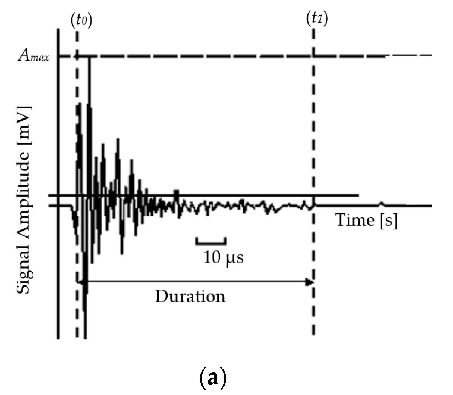
Each channel consists of an analog-to-digital converter (ADC) module with a sampling rate of 10 mega-samples per second, which is adequate to measure frequency components up to 1 MHz, covering satisfactorily the typical frequency range of broadband PZT transducers. However, in the present application, the use of highly sensitive resonant transducers (with resonant frequency of 63 kHz) appeared more appropriate. During AE monitoring, the typical frequencies of signals emitted from micro-cracks and sources, generated in materials such as concrete and masonry, range between 50 kHz and 250 kHz. The sampling rate of the AE device (10 Ms/s) is between 200 and 50 times the AE signal frequency correlated to the damage evolution. In Figure 7, a typical AE signal is reported. The AE equipment used in the present paper allowed us to set the appropriate threshold value due to the monitored structure and the environmental conditions. As regards the amplitudes, the instrumentation used permitted the determination of two different modalities in the definition of the threshold values, beyond which the signal is effectively recognized and recorded (see Fig. 7a). The signal threshold value is normally defined in a range from 50 µV to 100 mV. The great variability on the thresholds that can be set by the AEMission device allowed for the definition of the most appropriate one for each sensor set, based on the condition in which the monitoring is operating [6,7,8,9,10,20]. The background noise, in fact, can be generated in different sources and external conditions. The causes of the noises can be mechanical, electromagnetic, or generated by human action or environmental conditions. Generally, there is a tendency to maintain a low threshold level in order to avoid in the cutting of a large amount of significant data. In this way, it will be possible to subsequently filter the data during the post-processing phase. On the other hand, the preset thresholds for the acquisition must be high enough to avoid saturation of the acquisition memories due to the effect of repetitive signals and due to the background noise. The threshold methods used in the various cases were implemented in the software of the device used and reported by the authors in recent publications [20].
The AE equipment automatically performs different kinds of analyses. The first parameter is represented by the cumulative number of AE signals N, detected during the monitoring time. In addition, the time dependence of the structural damage observed during the monitoring period, identified by parameter η, can also be correlated to the rate of propagation of the micro-cracks. If we express the ratio of the cumulative number of AE counts recorded during the monitoring process, N, to the number obtained at the end of the observation period, Nd, as a function of time, t, we get the damage versus time dependence [6,7,8,9,10,24,25,26]:
where E and Ed represented the energy dissipation during micro-crack propagation in general and with respect to the monitoring time. By working out the βt exponent from the data obtained during the observation period, we can make a prediction regarding the structural stability conditions.
Damage assessment in the structure may be also investigated by the statistical distribution of the AE signal magnitudes fitted by the Gutenberg–Richter (GR) law. The b-value is usually computed using the cumulative frequency magnitude distribution data and applying the GR law. By analogy with seismic phenomena, in the AE technique, the magnitude may be defined as follows [17]:
where Amax is the amplitude of the signal expressed in μV and f(r) is a correction coefficient whereby the signal amplitude is taken to be a decreasing function of the distance r between the source and the AE sensor. According to Gutenberg–Richter’s empirical law [17],
that can be re-written as:
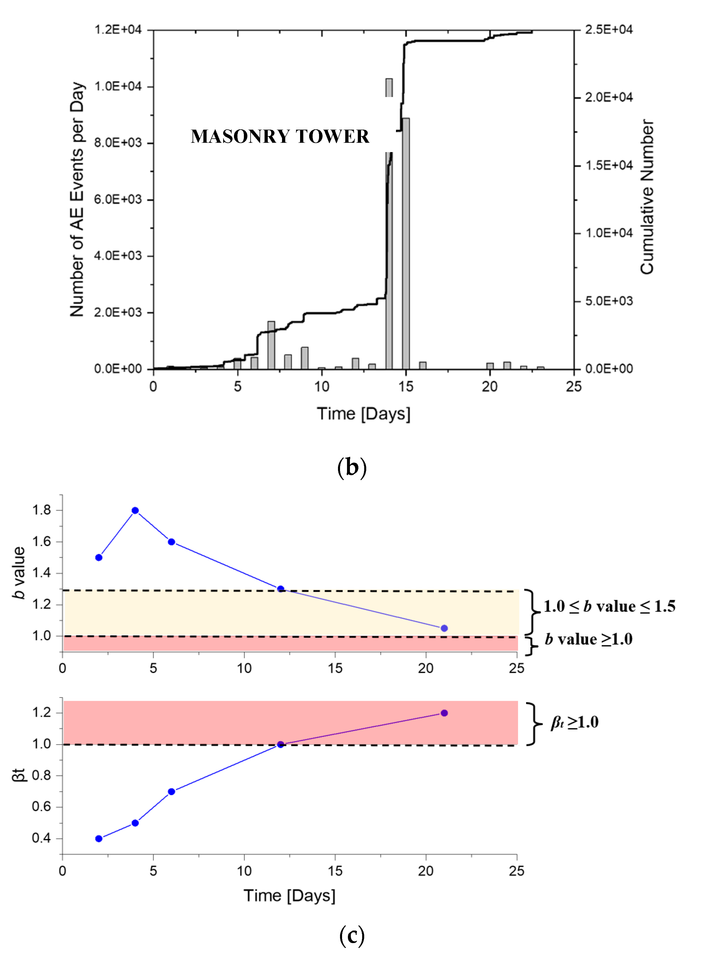
where n is the cumulative number of earthquakes (AE events) with magnitude ≥ m in a given area and a within specific time range, whilst a and b are positive constants varying from a region to another and from a time interval to another. The damage evolution in the masonry structure of the tower is described by the evaluation of the cumulative number of AE and by different parameters able to predict the time dependence of damage, including the b-value [6,7,8,9,10,13,14]. In particular, since environmental disturbances have been minimized and instrumental noises have been filtered out, the b-value analysis showed a downward trend to values compatible with the growth of localized macro-cracks in the south side of the tower. The analysis denounced the presence of a damage processes mainly localized at the base of the monitored structure between levels 2 and 3. The extension of the monitoring periods and the investigation of different segments are strongly recommended to assess the stability of the monument [24,25,26].
The analysis of the b-value has been widely used for the application of AE analysis. In particular, during the last few decades, very important results were achieved for concrete structures using b-value and improved b-value by Shiotani et al. [27,28]. In present paper, in order to carry out an accurate study, the disturbances of the environment and the noise filters of the instrumentation have been optimized. In particular, a filtering on amplitude signal levels and frequency values is adopted for the AE time series. The b-value trend was obtained working on time windows containing at least 100 AE. Signals with repetitive frequency values or too far from the typical range proper of the frequency of the damage source generation in these types of materials have been discarded. In particular, it is interesting to note that the b-value showed a decreasing trend that is compatible with the growth of macro-cracks localized in the south side of the tower between the second and the third level, in correspondence of the portion of the monitored structure. After 12 monitoring days, the b-value trend entered the 1.5 < b-value > 1.0 phase, corresponding to a critical condition (Figure 7c).
In this phase, the localized point started to be found by the triangulation procedure as stated in the following. After 21 monitoring days, the trend approached the local collapse condition 1.0 < b-value (Figure 7c). This phase was correlated with the intensification of the localized point of the damage sources (Figure 8), in correspondence of the evolution of active cracks (Figure 8a,b). Furthermore, as reported in Figure 7c, the growth of the βt toward values higher than 1.0 in correspondence with the decrease in the b-value highlighted the instability of the crack growth process. As mentioned before, the localization procedure was employed to evaluate the source damage position and the diffusion of the cracking pattern. Localization is one of the most used analysis in AE monitoring. The AE localization technique has been widely applied in laboratory and in situ tests, as well as, has been performed with different methods in order to improve the results accuracy [29,30,31,32,33,34,35,36,37,38,39,40,41]. In this second stage (low b-value and higher βt,) in fact, the formation of micro-cracks in a 3D space is analyzed, and the triangulation technique was applied to signals recorded by at least five sensors falling into time intervals sufficiently small (50 µs). Thus, with this procedure, it is possible to define both the position of the micro-cracks in the volume and the speed of longitudinal P-waves transmission in the medium. Having denoted with ti the arrival time at a sensor Si of an AE event generated at point S and at time t0’
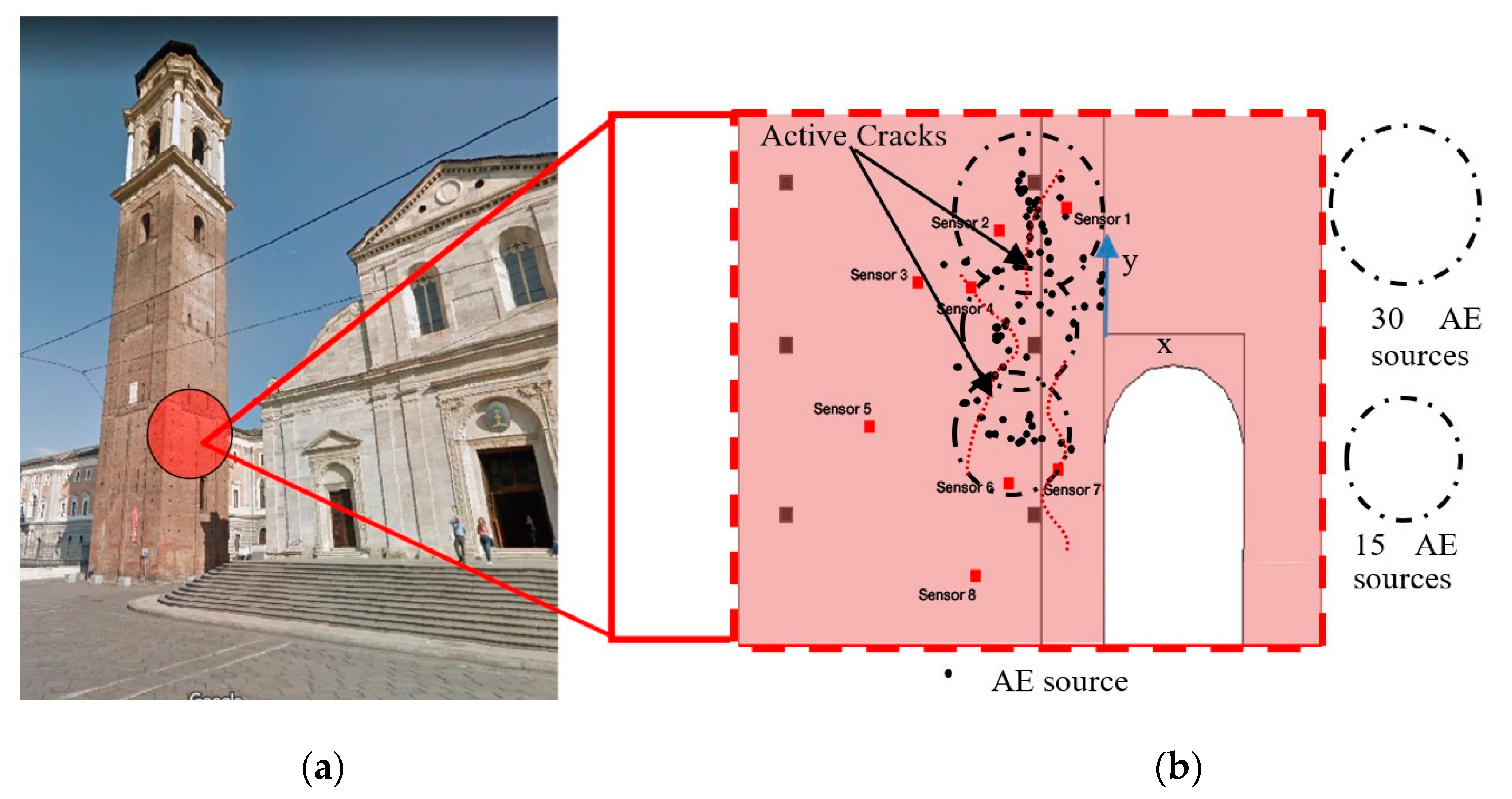
the distance between Si and source S, in Cartesian coordinates, and assuming the material to be homogenous, the path of the signal is given by |S − Si| = v(ti − t0). If the same event is observed from another sensor Sj at time tj: |S − Sj| − |S − Si| = v(ti − t0). Assuming the arrival times of the signals and the positions of the two sensors to be known, the last is an equation with four unknowns—x, y, z, and v. Hence, the problem of the localization of S is determined if it is possible to write a sufficient number of equations of that type, i.e., when the same AE event is identified by at least five sensors. If this did not occur, it would be necessary to adopt simplifying assumptions to reduce the degrees of freedom of the problem, such as, for instance, imposing the speed of transmission of the signals or having the AE source lie on predetermined plane. For the analysis carried out in the present research, three-dimensional localizations with at least five sensors were performed. In particular, Figure 8a and Table 6 indicate the position where the sensors were applied, (Figure 8b) the result of the localization with the source points projected on the surface of the facade, (Figure 8c) the relationship with the main results of the numerical model, and (Figure 8d) the detection of damage together with the crack pattern on the same portion of the structure. The localization procedure is based on the principles recently reported by the same authors concerning the signal accuracy [20]. Finally, according to the steps described in the previous section, the sources of AE events were localized. The localized points have been indicated with black points, for a total of 62 AE sources. In the figure, three circles are reported in correspondence to the center of the AE source clusters. Two levels of cluster are reported with circle radii proportional to the number of AE source inside the areas (see Figure 8b). In Figure 8d, the map of surface erosions, masonry gaps, surface damage, and cracks was reported. The AE localization allowed us to identify the portions of the masonry where active and growing cracks were concentrated (Figure 8b). These areas are also those where the highest values in compressive stresses were observed through the numerical model during the static calculus (Figure 8c).
|S − Si| = [(x − xi)2 + (y − yi)2 + (z − zi)2]1/2
The second part of the Bell Tower subjected to the AE monitoring is the timber structure sustaining the bells, positioned inside the bell cell at the top of the tower (see Figure 9). In this case, the wooden structure supporting the bells was monitored with an eight-channel acoustic emission data acquisition system to evaluate the evolution of the cracking pattern evolution over the monitoring time (see Table 7 for the sensor positioning). The sensors were positioned in the wood frame sustaining the heaviest bells, as shown in Figure 8. The structure was monitored for a period of time equal to one month; in particular, the monitoring was carried out from 8 August to 8 September 2019.
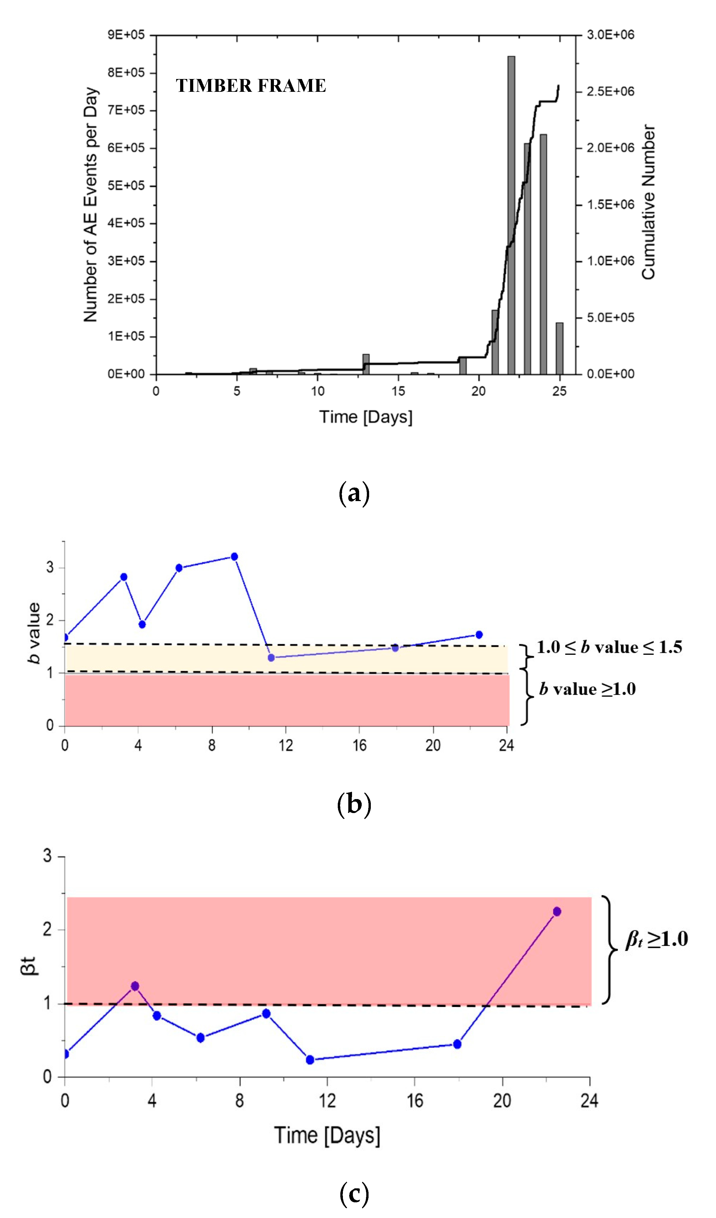
The analysis of the data extracted from the AE device followed similar steps previously observed for the monitoring of the masonry structure of the Bell Tower (see Figure 10). Figure 10a shows the AE cumulative number recorded during the monitoring period and the number of EA events for each day for the timber frame. The b-value trend was obtained working on time windows containing at least 100 AE. As observed in the case of the masonry structure, the b-value assumed numbers greater than 1.5, in correspondence with the first monitoring phase (first 10 monitoring days). After 11 days, the analysis results entered the critical band 1.5 < b-value > 1.0 (Figure 10b). In addition, as seen in Figure 10c, the βt exponent showed an evident growth after 17 monitoring days. This increment is not perfectly correlated with the b-value decrease, but the two phases can be considered just in correspondence.
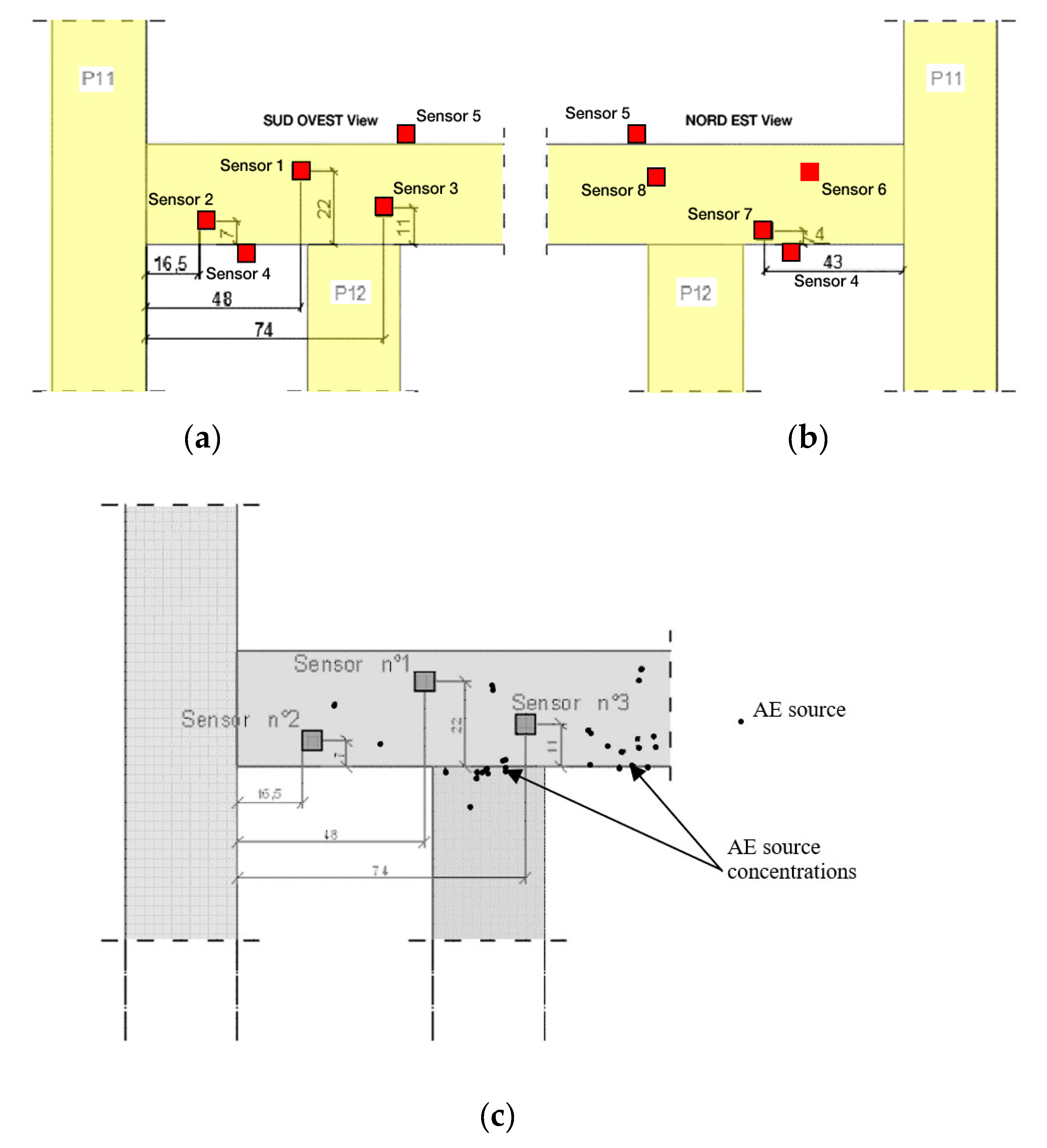
Finally, the sources of AE events were localized. The position of the sensors and the localized sources are shown in Figure 11a,b. The localized points have been indicated with black points, for a total of 24 AE sources. In this Figure, two circles are reported in correspondence to the barycenter of AE source clusters. Two levels of cluster are reported with circle radii proportional to the number of AE source inside the areas. The results of the AE localization, together with the b-value trend, made it possible to identify the column-beam joint and the portion of the beam close to the pin of the big bell as a portion of the wood frame affected by crack formation and damage growth.
4. Correlation between the Structural Monitoring and the Seismic Activity
A recently published research article analyzed different seismic sequences and proposed a methodology to establish if a series of earthquake events is related to a succession (aftershocks), or if it is belonging to events of a preliminary phase before a main event (foreshock) [21]. The parameter used for this real-time discrimination between foreshock and aftershock phases, reported in the original paper, is the behavior of the average value calculated on the b-value of the seismic time series. [21]. The study of the seismic sequences was applied principally to the Amatrice and the Norcia earthquake activity in 2016 [21]. It was possible to observe how the average value undergoes a growth, approximately equal to 20%, following a “main event.” On the contrary, in the time window between events of similar intensity, an evident reduction in the average value of the b-value is observed (foreshock), which therefore contributes to find a forecast parameter with respect to a very probable new main event [21]. Based on the approach described above, similar results were obtained in the b-values trends computed by the seismic events recorded in the area near to the monitoring site (Turin) in a circular portion of territory with radius = 100 km around the tower. In addition, a correlation between the AE and the seismic data were found based on the theoretical and experimental observations recently reported in some works dedicated to AE monitoring of monumental structures in seismic active regions [18]. First of all, since the monitored structure falls in an area characterized by less seismic activity, the trend of the b-value of the seismic events was studied in order to verify that, even on sequences characterized by lower magnitudes, the behavior observed by Guglia and Weimer (2019) [21] can be used also in this case to distinguish between the “foreshocks” and “aftershocks” phases.
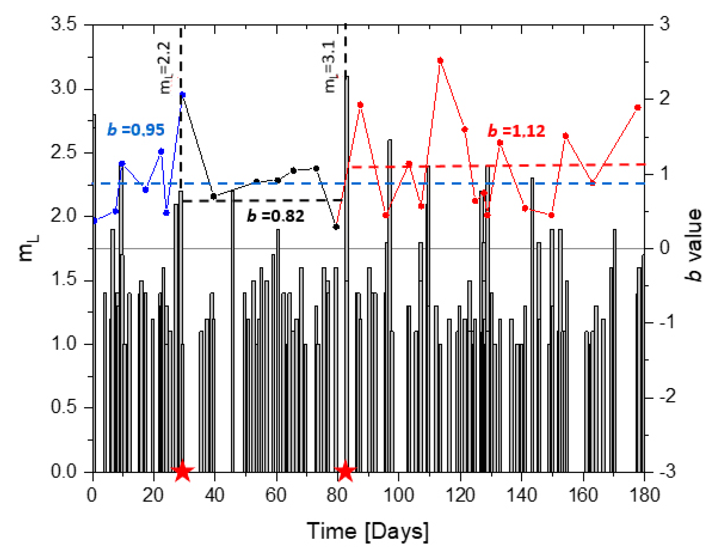
Therefore, the earthquakes occurred in an area surrounding the bell tower of the Cathedral of Turin were considered in a six-month time window. The events selected are those that occurred between 15 March and 14 September 2018; the monitoring performed by the AE technique on the structures of the Cathedral is located in the final part of the time window here considered. The reference events evaluated in the period have the following characteristics mL (local magnitude): 2.2 occurred on 12 April 2018 with the epicenter in Massello, a region far from Turin about 86 km, and mL: 3.1 occurred on 5 June 2018, with the epicenter localized between Italy and France (about 90 km from Turin). The results confirmed (for time series with a lower range in the magnitude levels) the evidence reported by Gulia and Wiemer (2019) [21]. In particular, in Figure 12, the trend of the b-value is reported together with the local magnitude of the seismic events considered. The average value of the b-values before the event considered as the “anticipator” is equal to 0.95, following the seismic event with mL: 2.2, there is an evident reduction in the average value. The average b-value number decreased of about 15% down to 0.82. Following the main event (mL: 3.1), which occurred about 50 days after the reduction of the average b-value, an increase of 30% was recorded, and the average b-value was equal to 1.12. The evidence reported in Figure 12 represented a good confirmation that the procedure recently proposed for regions characterized by an intense earthquake activity (high magnitude levels) can be successfully used also for region where the seismic level is lower (Piedmont, northwest of Italy).
In order to verify the hypotheses presented by the authors in the correlation between AE and seismic data, the historical time series of the seismic data were reported for two time windows containing the periods of the AE monitoring, performed on the tower structure and then in the timber structure positioned in the bell cell. The data related to the seismic time series were assessed and obtained from the Italian National Institute of Geology and Volcanology (INGV) that reported all the seismic events recorded by the National Seismic Network (http://terremoti.ingv.it/instruments). The following reduction of the local magnitudes based on the distance between the monitored site and the epicenter according to the following report is assumed:
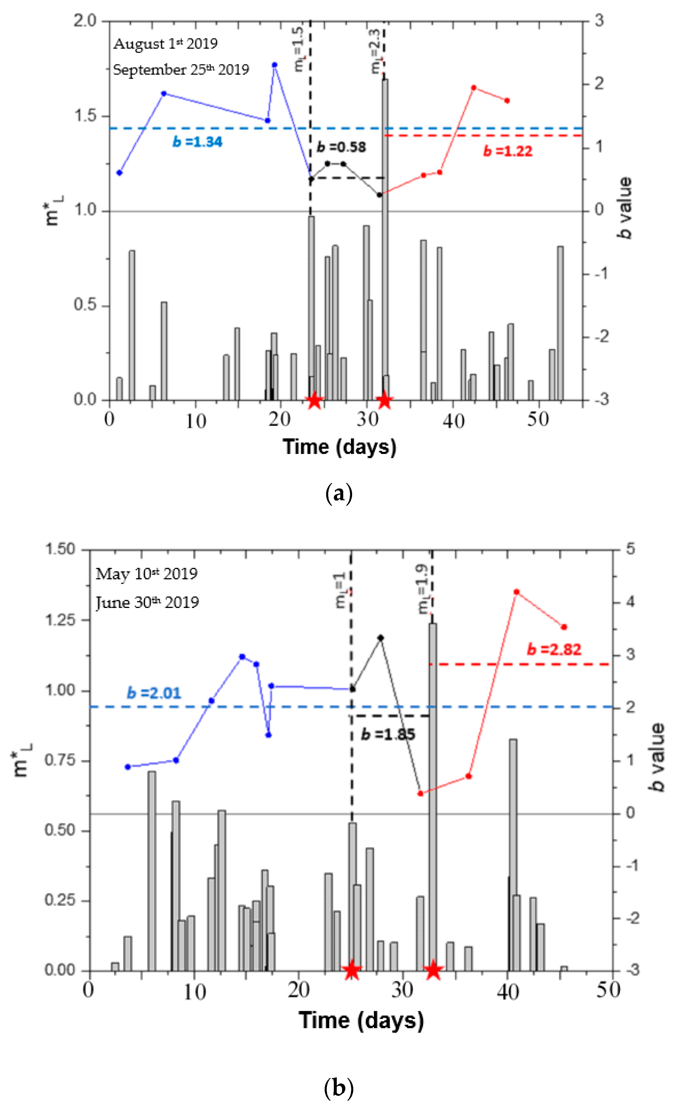
where mL* is the reduced local magnitude; mL is the actual local magnitude and d is the distance, measured in km, between the epicenter and the Bell Tower of the Turin Cathedral. In Figure 13 the two seismic time series were represented together with the variations of the average b-values.
These variations trends resulted particularly evident for both the two considered periods (10 May 2018–30 June 2018 and 1 August 2019–25 September 2019). For each period, two couples of events were recognized, each of them formed by one anticipant and one main event (the anticipant and the main events are distinguished by stars on the x-axis of the graph). The average values of the b-value before the anticipating events are 1.34 and 2.01 for the two periods, respectively (see Figure 13a,b). The reduced local magnitudes for the two anticipants are mL* = 1.5 (1 June 2018, Inverso Pinasca, 44°57′ N 7°13′ E, near Turin); and mL* = 1.0 (24 August 2019, Torre Pellice, 44°49′ N 7°14′ E). After these two events two phases, the first of about seven days and the second of about eight days with average b-values of 0.58 and 1.85 were observed for the two time windows. After these intervals, the expected seismic main events mL* = 2.3 and mL* = 1.9 took place (Figure 13a,b). These two events were both anticipated by the previously mentioned series where the average b-values encountered reductions of 56% and 8%. After the occurrence of the two events recognized as main events, the b-values trends returned to grow significantly—the average b-values were 1.22 for the first time window and even 2.82 for the second (Figure 13a,b). The evidence here reported is useful to understand that the discrimination criterion reported by Guglia and Weimer (2019) [21] can be applied to seismic series with reduced magnitude values (0.5 < mL < 3) and also in the case of rescaled values that follow the reduction rule reported in Equation (8).
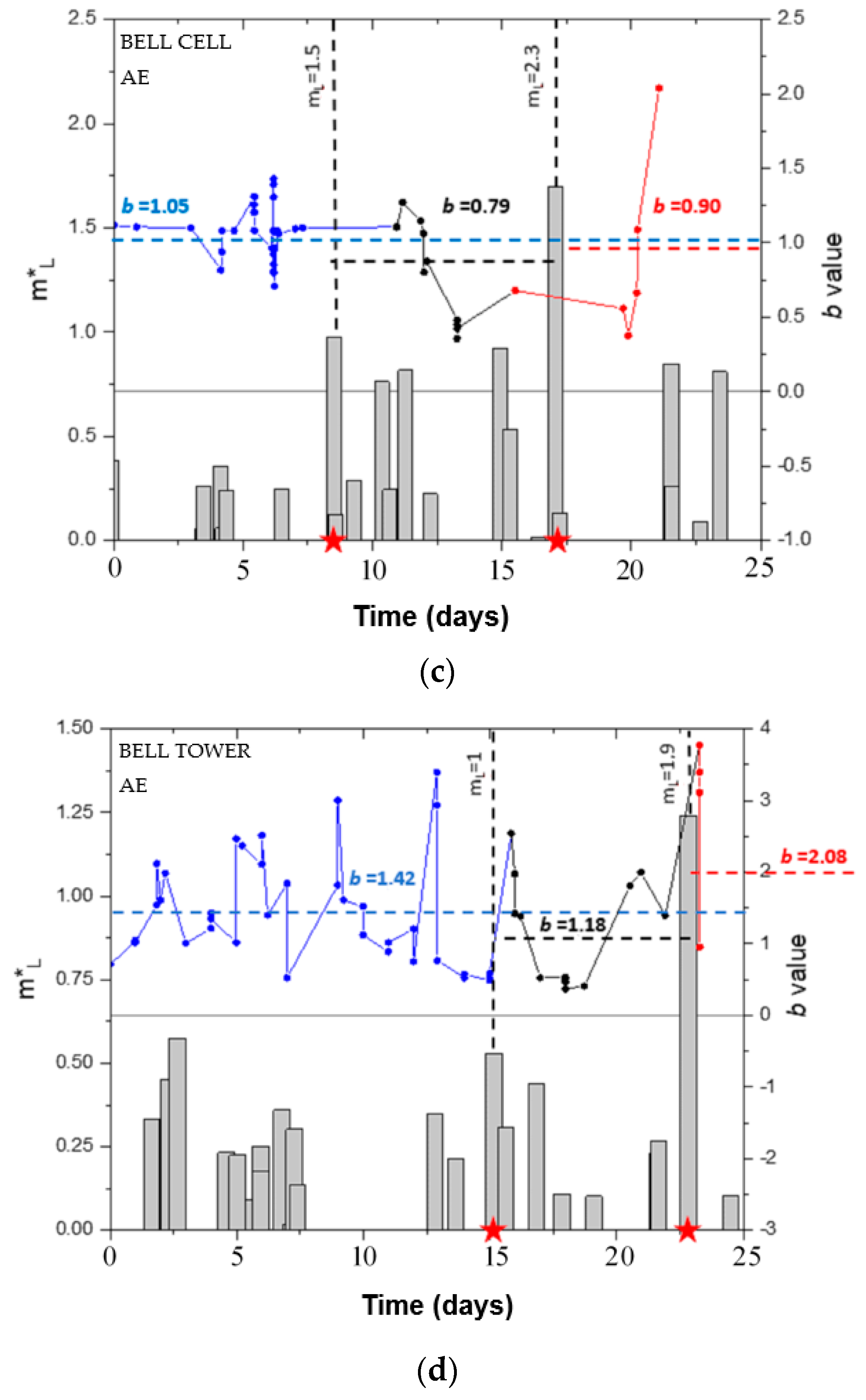
Similar considerations can be proposed in the case of AEs. Furthermore, the possibility to evaluate a close correlation between the regional seismic activity and the AE monitoring results was recently presented [18]. First of all, the AE data series were acquired for the two periods considered above, and the verification, if the couples of events previously recognized were in the AE monitoring intervals, was done. At this point, we proceeded to remove from the AE data series all signals used to determine the sources of damage through the AE localization. In this way, all the AE data directly related to the structural damage of the masonry and the wood structures were excluded from the AE time series used to evaluate the correlation between AE and seismic activity. In order to verify the original hypotheses, the historical time series of the AE data were reported for two 25-day intervals contained in the two time windows presented. In Figure 13, the seismic time series are represented together with the variations of the AE average b-values detected on the structures of the tower. In this case, the variations trends resulted particularly evident for both the two considered periods. The average values of the AE b-value before the anticipant events are 1.05 and 1.42 for the two anticipating intervals, respectively (see Figure 13c,d). After the two anticipating events, average AE b-values of 0.79 and 1.18 were observed for the two intervals before mL* = 2.3 and mL* = 1.9, respectively (Figure 13c,d). These two events were both anticipated by the previously mentioned series where the average b-values encountered reductions of 24% and 25%. After the occurrence of the two events recognized as main events, the b-values trends returned to grow significantly—the average b-values were 0.90 for the first time window and even 2.08 for the second (Figure 13c,d). The evidence here reported are very important and denounced the possibility of using the AE average b-values to offer a discrimination of the foreshock and aftershock period in a region affected by seismic activity.
5. Conclusions
This paper presents the representative case study of the monitoring of the Turin Cathedral bell tower. First of all, the damage evolution in a portion of the external bearing walls is described by the evaluation of the cumulative number of AE and by different parameters able to predict the time dependence of the damage. In particular, the b-value analysis showed a decreasing trend down to values in the critical phase well-matching with the growth of the localized macro-cracks in the masonry portion near to the base of the tower. The AE results were found in good agreement with the numerical simulations implemented by Midas software (CSP Fea Engineering, Padova, Italy). To obtain an improvement in the AE data analysis, signals with repetitive frequency or with values too distant from the typical range of the damage source generation in these types of materials were discarded. Furthermore, the growth of the βt toward values higher than 1.0 evidenced the instability of the damage process.
The results of the localized procedure were detected just at the end of the monitoring and in correspondence of the critical values of b-value and βt. After this first monitoring activity, the AE cumulative numbers were also detected during the monitoring of the wood frame sustaining the tower bells positioned in the ancient cell of the tower. As observed in the case of the masonry structure, the b-value assumed values greater than 1.5, in correspondence of the first phase. After 11 days, the analysis results entered the critical band, in correspondence to the localization of the AE sources found for the wood beam sustaining the heavier bell. For the wood frame monitoring, the βt exponent showed an evident growth after 17 monitoring days.
The b-value analyses were computed also at the seismic scale. The correlation between the structural behavior and the seismic activity was studied by comparing the b-value, obtained by AE signal detection on the structures of the tower, and the regional seismic activity. Concerning the correlation between the AE monitoring and regional seismic activity, a recent innovative analysis on different seismic sequences obtained surprising results. A new methodology able to discriminate foreshock and aftershocks earthquake time series was proposed. In the present paper, based on this approach, a correlation was obtained between the b-values computed by the seismic events recorded in the area near to the monitoring site (Turin), in a circular portion of territory with radius = 100 km around the tower. The first result of the present research regarded the confirmation that the analysis proposed by Guglia and Weimer (2019) [21] can be applied in seismic territory characterized by a low level of seismic magnitudes. The second evidence is related to the AE average b-values. Also, in this case, these variation trends were particularly evident for the considered periods. The average values of the AE b-value before the anticipant events are 1.05 and 1.42 for the two anticipating intervals. respectively. After the two anticipating events, the average AE b-values of 0.79 and 1.18 were observed for the two intervals before the main events. These two events were both anticipated by the previously mentioned series where the average b-values encountered reductions of 24% and 25%. The present study represents the first evidence that the AE average b-value analysis can be used, in addition to a seismic time series, as a robust parameter to discriminate between foreshock and aftershock intervals.
Author Contributions
Conceptualization, A.M.B. and D.M.; Methodology, A.M.B.; Software, D.M.; Validation, A.M.B.; Formal Snalysis, A.C.; Investigation, A.M.B.; Resources, A.M.B.; Data Curation, A.M.B.; Writing—Original Draft Preparation, A.M.B.; Writing—Review and Editing, A.M.B. and A.C.; Visualization, D.M.; Supervision, A.C.; Project Administration, A.C.; Funding Acquisition, A.C. All authors have read and agreed to the published version of the manuscript.
Funding
This research received no external funding.
Acknowledgments
Special thanks are due to Eng. Davide Perrone for the numerical analysis and the AE data elaboration.
Conflicts of Interest
The authors declare no conflict of interest.
References
- Aggelis, D.G.; Mpalaskas, A.; Matikas, T.E. Investigation of different fracture modes in cement-based materials by acoustic emission. Cem. Concr. Res. 2013, 48, 1–8. [Google Scholar] [CrossRef]
- Aki, K. A probabilistic synthesis of precursory phenomena. In Earthquake Prediction; Simpson, D.W., Richards, P.G., Eds.; American Geophysical Union (AGU): Washington, DC, USA, 2013; pp. 566–574. [Google Scholar]
- Bak, P.; Tang, C. Earthquakes as a self-organized critical phenomenon. J. Geophys. Res. Space Phys. 1989, 94, 15635–15637. [Google Scholar] [CrossRef] [Green Version]
- Ohtsu, M.; Okamoto, T.; Yuyama, S. Moment tensor analysis of acoustic emission for cracking mechanisms in concrete. ACI Struct. J. 1998, 95, 87–95. [Google Scholar]
- Bak, P.; Christensen, K.; Danon, L.; Scanlon, T. Unified Scaling Law for Earthquakes. Phys. Rev. Lett. 2002, 88, 178501-1–178501-4. [Google Scholar] [CrossRef] [PubMed] [Green Version]
- Carpinteri, A.; Lacidogna, G. Structural Monitoring and Integrity Assessment of Medieval Towers. J. Struct. Eng. 2006, 132, 1681–1690. [Google Scholar] [CrossRef]
- Carpinteri, A.; Lacidogna, G. Damage evaluation of three masonry towers by acoustic emission. Eng. Struct. 2007, 29, 1569–1579. [Google Scholar] [CrossRef]
- Carpinteri, A.; Lacidogna, G. Acoustic Emission and Critical Phenomena: From Structural Mechanics to Geophysics; CRC Press: Boca Raton, FL, USA, 2008. [Google Scholar]
- Anzani, A.; Binda, L.; Carpinteri, A.; Lacidogna, G.; Manuello, A. Evaluation of the repair on multiple leaf stone masonry by acoustic emission. Mater. Struct. 2007, 41, 1169–1189. [Google Scholar] [CrossRef]
- Carpinteri, A.; Lacidogna, G.; Manuello, A.; Niccolini, G. A study on the structural stability of the Asinelli Tower in Bologna. Struct. Control Health Monit. 2015, 23, 659–667. [Google Scholar] [CrossRef]
- Costa de Beauregard, C.A. Familles historiques de Savoie; Les Seigneurs de Compey: Puthod, Chambéry, France, 1884. [Google Scholar]
- Gentile, G. Io maestro Meo di Francescho Fiorentino. Documenti per il cantiere del Duomo di Torino. In Romano, Giovanni, Domenico della Rovere e il Duomo nuovo di Torino: Rinascimento a Roma e in Piemonte; Cassa di risparmio di Torino: Torino, Italy, 1990; pp. 107–200. [Google Scholar]
- Niccolini, G.; Manuello, A.; Marchis, E.; Carpinteri, A. Signal frequency distribution and natural-time analyses from acoustic emission monitoring of an arched structure in the Castle of Racconigi. Nat. Hazards Earth Syst. Sci. 2017, 17, 1025–1032. [Google Scholar] [CrossRef] [Green Version]
- Masera, D.; Bocca, P.; Grazzini, A. Frequency Analysis of Acoustic Emission Signal to Monitor Damage Evolution in Masonry Structures. J. Phys. Conf. Ser. 2011, 305, 012134. [Google Scholar] [CrossRef]
- Omori, F. On Aftershocks. Rep. Imp. Earthquake Invest. Comm. 1894, 2, 103–109. [Google Scholar]
- Richter, C.F. Elementary Seismology; W. H. Freeman and Company: San Francisco, CA, USA; London, UK, 1958. [Google Scholar]
- Carpinteri, A.; Lacidogna, G.; Niccolini, G.; Puzzi, S. Critical defect size distributions in concrete structures detected by the acoustic emission technique. Meccanica 2007, 43, 349–363. [Google Scholar] [CrossRef]
- Carpinteri, A.; Lacidogna, G.; Niccolini, G. Acoustic emission monitoring of medieval towers considered as sensitive earthquake receptors. Nat. Hazards Earth Syst. Sci. 2007, 7, 251–261. [Google Scholar] [CrossRef] [Green Version]
- Lacidogna, G.; Manuello, A.; Niccolini, G.; Carpinteri, A. Acoustic emission monitoring of Italian historical buildings and the case study of the Athena temple in Syracuse. Arch. Sci. Rev. 2012, 58, 1–10. [Google Scholar] [CrossRef]
- Carpinteri, A.; Xu, J.; Lacidogna, G.; Manuello, A. Reliable onset time determination and source location of acoustic emissions in concrete structures. Cem. Concr. Compos. 2012, 34, 529–537. [Google Scholar] [CrossRef]
- Gulia, L.; Wiemer, S. Real-time discrimination of earthquake foreshocks and aftershocks. Nature 2019, 574, 193–199. [Google Scholar] [CrossRef]
- Binda, L.; Bertocchi, E.; Trussardi, D. Torri in muratura: Una metodologia per la valutazione della sicurezza. Recupero Conservazione 1997, 18, 26–34. (In Italian) [Google Scholar]
- Available online: https://www.lunitek-ssm.com/ (accessed on 1 February 2020).
- Niccolini, G.; Durin, G.; Carpinteri, A.; Lacidogna, G.; Manuello, A. Crackling noise and universality in fracture systems. J. Stat. Mech. Theory Exp. 2009, 2009, P01023. [Google Scholar] [CrossRef] [Green Version]
- Niccolini, G.; Bosia, F.; Carpinteri, A.; Lacidogna, G.; Manuello, A.; Pugno, N.M. Self-similarity of waiting times in fracture systems. Phys. Rev. E 2009, 80, 26101/1–26101/6. [Google Scholar] [CrossRef] [Green Version]
- Carpinteri, A.; Lacidogna, G.; Manuello, A. Damage Mechanisms Interpreted by Acoustic Emission Signal Analysis. Key Eng. Mater. 2007, 347, 577–582. [Google Scholar] [CrossRef]
- Shiotani, T.; Yuyama, S.; Li, Z.W.; Ohtsu, M. Application of AE improved b-value to quantitative evaluation of fracture process in concrete materials. J. Acoust. Emiss. 2001, 19, 118–132. [Google Scholar]
- Shiotani, T.; Fujii, K.; Aoki, T.; Amou, K. Evaluation of progressive failure using AE sources and improved b-value on slope model test. Prog. Acoust. Emiss. VII JSNDI 1994, 7, 529–534. [Google Scholar]
- Ohtsu, M.; Kaminaga, Y.; Munwam, M.C. Experimental and numerical crack analysis of mixed-mode failure in concrete by acoustic emission and boundary element method. Constr. Build. Mater. 1999, 13, 57–64. [Google Scholar] [CrossRef]
- Berkovits, A.; Fang, D. Study of fatigue crack characteristics by acoustic emission. Eng. Fract. Mech. 1995, 51, 401–416. [Google Scholar] [CrossRef]
- Tobias, A. Acoustic-emission source location in two dimensions by an array of three sensors. Non-destr. Test. 1976, 9, 9–12. [Google Scholar] [CrossRef]
- Asty, M. Acoustic emission source location on a spherical or plane surface. NDT Int. 1978, 11, 223–226. [Google Scholar] [CrossRef]
- Barat, P.; Kalyanasundaram, P.; Raj, B. Acoustic emission source location on a cylindrical surface. NDT E Int. 1993, 26, 295–297. [Google Scholar] [CrossRef]
- Dong-Jin, Y.; Kim, Y.H.; Oh-Yang, K. New algorithm for acoustic emission source location in cylindrical structure. J. Acoust. Emiss. 1992, 9, 237–242. [Google Scholar]
- Landau, B.; West, M. Estimation of the source location and the determination of the 50% probability zone for an acoustic source locating system (SLS) using multiple systems of 3 sensors. Appl. Acoust. 1997, 52, 85–100. [Google Scholar] [CrossRef]
- Choi, Y.-C.; Kim, Y.-H. Impulsive sources localization in noisy environment using modified beamforming method. Mech. Syst. Signal Process. 2006, 20, 1473–1481. [Google Scholar] [CrossRef]
- Maochen, G. Analysis of source location algorithms Part I: Overview and non-iterative methods. J. Acoust. Emiss. 2003, 21, 14–28. [Google Scholar]
- Ernst, R.; Dual, J. Acoustic emission localization in beams based on time reversed dispersion. Ultrasonics 2014, 54, 1522–1533. [Google Scholar] [CrossRef] [PubMed]
- Grabec, I.; Kosel, T.; Mužič, P. Location of continuous AE sources by sensory neural networks. Ultrasonics 1998, 36, 525–530. [Google Scholar] [CrossRef]
- Ohtsu, M.; Ono, K. The generalized theory and source representations of acoustic emission. J. Acoust. Emiss. 1986, 5, 124–133. [Google Scholar]
- Ono, K.; Ohtsu, M. A generalized theory of acoustic emission and Green’s functions in a half space. J. Acoust. Emiss. 1984, 3, 27–40. [Google Scholar]
Figure 1.
Architectural complex of the Cathedral with the bell tower in the front and the dome erected by G. Guarini: (a) on the backside; (b) view of the isolated bell tower from the other side
Figure 1.
Architectural complex of the Cathedral with the bell tower in the front and the dome erected by G. Guarini: (a) on the backside; (b) view of the isolated bell tower from the other side

Figure 2.
Tall masonry building in Turin and parts constituting the bell tower. (a) The bell tower is the third tallest masonry building in the city (63 m); (b) The tower is subdivided into different parts—the stem and the bell cell are constituted by different materials and were erected in different times and by different building techniques.

Figure 3.
The FEM: (a) The bell tower is made with different materials and different building techniques (sack masonry). (b) Chains have also been inserted within the model in correspondence with the "key heads" observable from the outside. The loads of the various elements were assessed by multiplying their thickness by the specific weight of the materials. The different dead loads were associated to the different levels and structural elements. (c) Axonometric cross-section of the tower.

Figure 4.
Compressive stress σ for different ancient tall masonry towers in Italy [22]. The maximum stress is reported as a function of the ratio between the height and the maximum depth of the bearing wall of the structure.
Figure 4.
Compressive stress σ for different ancient tall masonry towers in Italy [22]. The maximum stress is reported as a function of the ratio between the height and the maximum depth of the bearing wall of the structure.

Figure 5.
Portion of the structures were the maximum compressive stress was localized. The compressive stress value at the base of the tower is 0.95 MPa.
Figure 5.
Portion of the structures were the maximum compressive stress was localized. The compressive stress value at the base of the tower is 0.95 MPa.

Figure 6.
Representation of the modal analysis: (a,b) The two modes of the tower in the y and the x directions, represented by flexural modalities, (c) The third mode showing a torsional modality.
Figure 6.
Representation of the modal analysis: (a,b) The two modes of the tower in the y and the x directions, represented by flexural modalities, (c) The third mode showing a torsional modality.

Figure 7.
AE signal and AE results of the tower: (a) Typical received signal in the time domain during the acoustic emission (AE) monitoring. The AE equipment used in the present paper allow to set the appropriate threshold value due to the monitored structure and the environmental conditions. (b) Cumulative number of AE and AE count per day during the monitoring time. (c) b-value diagram representing the evolution of the damage, βt trend evolution during time.


Figure 8.
AE localization results. In (a), the portion of the masonry structure where the AE sensors were positioned. The localized points have been indicated with black points, for a total of 62 AE sources (b). Three circles are reported in correspondence to the center of AE source clusters. Two levels of cluster are reported with circle radius proportional to the number of AE source inside the areas. (c) The results of the numerical analysis reported the portion of the structure with higher compressive stress. (d) The same area is reported considering the crack position the erosion areas and the damaged surfaces.


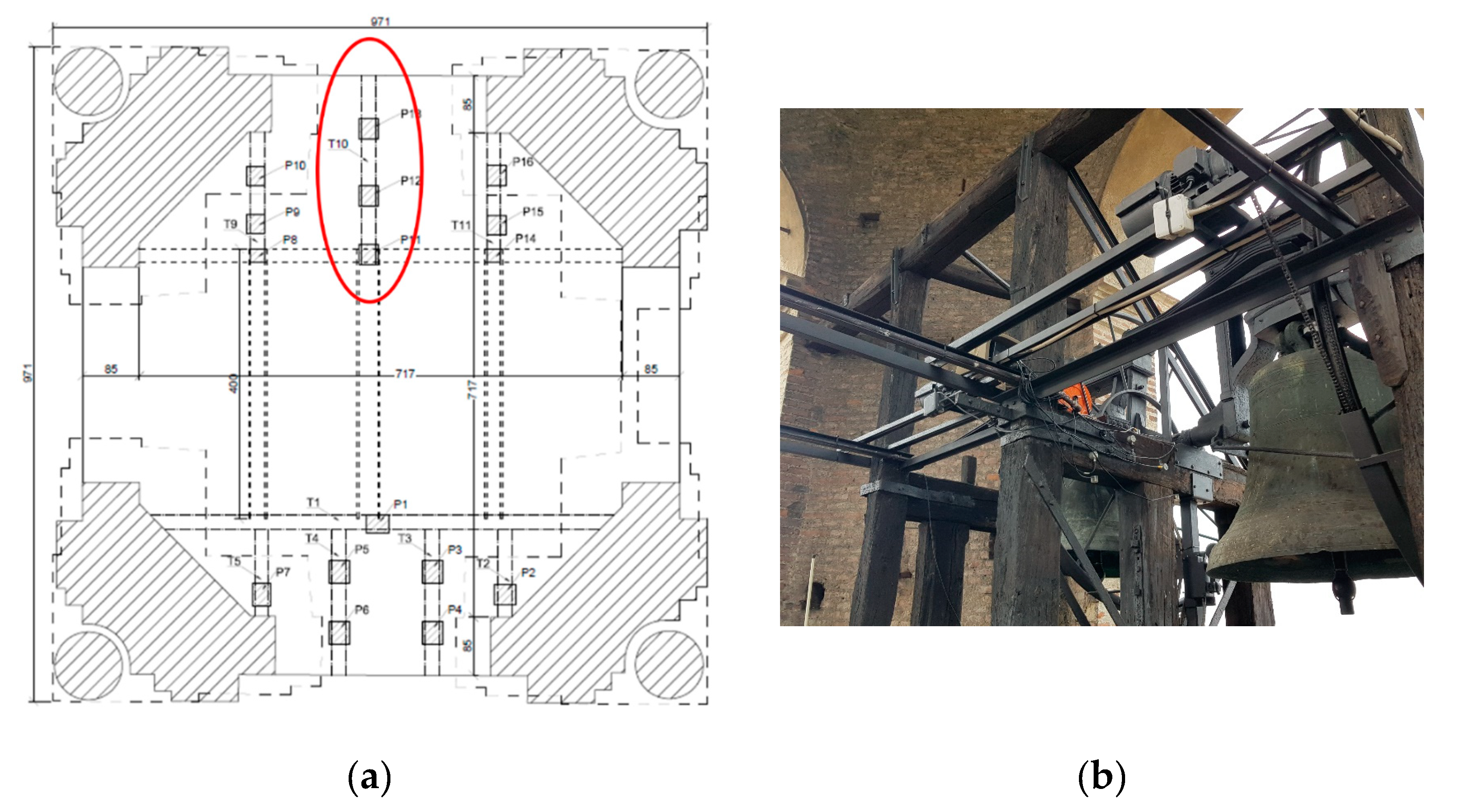
Figure 9.
Timber structure positioned inside the bell cell at the top of the tower: (a) Plan of the cell where the timber frame layout is reported. The monitored portion is localized. (b) AE sensors disposition on the wood frame.
Figure 9.
Timber structure positioned inside the bell cell at the top of the tower: (a) Plan of the cell where the timber frame layout is reported. The monitored portion is localized. (b) AE sensors disposition on the wood frame.

Figure 10.
Timber frame of the cell: (a) Cumulative number of AE and AE count per day during the monitoring time. (b) b-value diagram representing the evolution of the damage. (c) βt trend evolution.
Figure 10.
Timber frame of the cell: (a) Cumulative number of AE and AE count per day during the monitoring time. (b) b-value diagram representing the evolution of the damage. (c) βt trend evolution.

Figure 11.
AE localization results. In figure (a) and (b), the portion of the wooden frame where the AE sensors were positioned is showed, (c) The localized points have been indicated with black points, for a total of 24 AE sources.
Figure 11.
AE localization results. In figure (a) and (b), the portion of the wooden frame where the AE sensors were positioned is showed, (c) The localized points have been indicated with black points, for a total of 24 AE sources.

Figure 12.
The average b-values before the “anticipator” event (12 April 2018) is equal to 0.95. After this, an evident reduction in the average value equal to 15% is observed (average b-value = 0.82). The main event occurred about 50 days after (5 June 2018). After the mL: 3.1, no event with greater magnitude were registered for three months.

Figure 13.
The seismic time series are represented together with the variations of the AE average b-values detected on the structures of the tower: (a,b) b-value time series considering the seismic activity along 40-day time windows. In both the two cases the average b-values demonstrated an evident reduction in correspondence of foreshocks periods between the anticipating and the main event. (c,d) At the same time, the b-value time series have been computed for AE data and correlated to the seismic activity for a period of 25 days contained in the previous larger time intervals.


Table 1.
Material properties used in the model.
| Masonry type | fm [N/cm2] min – max | τ0 [N/cm2] min – max | E [N/mm2] min – max | G [N/mm2] min – max | γ [kN/m3] |
|---|---|---|---|---|---|
| Rubble Masonry | 100 – 182 | 2 – 3.2 | 690 – 1050 | 230 – 350 | 19 |
| Brick Masonry | 240 – 400 | 6 – 9.2 | 1200 – 1800 | 400 – 600 | 18 |
Table 2.
Vertical Loads.
| Element | Dead Load [daN] | Permanent Load [daN] | Variable Load [daN] |
|---|---|---|---|
| Vault 1 | 5.4 | 7.15 | 5 |
| Vault 2 | 5.4 | 6.24 | 5 |
| Vault 3 | 5.4 | 6.09 | 5 |
| Vault 4 | 5.4 | 5.61 | 5 |
| Wood floor | 0.69 | 0.00 | 5 |
| Roof | 0.98 | 0.98 | 1.23 |
Table 3.
Diameter and loads of the bells.
| Diameter [mm] | Load [daN] |
|---|---|
| 1410 | 2625.0 |
| 1100 | 1449.0 |
| 1000 | 997.5 |
| 800 | 609.0 |
Table 4.
Eigenvalue analysis.
| Mode n | Frequency | Period | |
|---|---|---|---|
| [rad/s] | [cycle/s] | [s] | |
| 1 | 2.5300 | 0.4027 | 2.4835 |
| 2 | 2.5687 | 0.4088 | 2.4460 |
| 3 | 10.208 | 1.6247 | 0.6155 |
Table 5.
Participating modal masses.
| Mode n | Tran-X | Tran-Y | Tran-Z | Rotn-X | Rotn-Y | Rotn-Z |
|---|---|---|---|---|---|---|
| Mass (%) | Mass (%) | Mass (%) | Mass (%) | Mass (%) | Mass (%) | |
| 1 | 31.452 | 25.482 | 0 | 18.006 | 22.289 | 0.001 |
| 2 | 25.427 | 31.456 | 0 | 22.288 | 18.054 | 0.001 |
| 3 | 15.108 | 0.220 | 0 | 0.187 | 12.861 | 19.762 |
Table 6.
Sensor positions on the south tower façade.
| Sensor n | Coordinate x [cm] | Coordinate y [cm] | Coordinate z [cm] |
|---|---|---|---|
| 1 | 21.51 | 123.5 | 15.00 |
| 2 | 59.15 | 111.05 | 0.00 |
| 3 | 10.208 | 83.63 | 0.00 |
| 4 | 105.53 | 81.50 | 0.00 |
| 5 | 133.15 | 7.50 | 0.00 |
| 6 | 51.50 | 22.01 | 0.00 |
| 7 | 26.00 | 15.82 | 15.00 |
| 8 | 72.20 | 71.48 | 0.00 |
Table 7.
Sensor positions on the wood frame sustaining the bells.
| Sensor n | Coordinate x [cm] | Coordinate y [cm] | Coordinate z [cm] |
|---|---|---|---|
| 1 | 48.15 | 22.50 | 0.00 |
| 2 | 18.51 | 7.50 | 0.00 |
| 3 | 73.26 | 11.00 | 0.00 |
| 4 | 31.29 | 0.00 | −7.00 |
| 5 | 80.14 | 29.89 | −7.00 |
| 6 | 26.50 | 19.90 | −15.00 |
| 7 | 43.69 | 04.00 | −15.00 |
| 8 | 76.70 | 18.90 | −15.00 |
© 2020 by the authors. Licensee MDPI, Basel, Switzerland. This article is an open access article distributed under the terms and conditions of the Creative Commons Attribution (CC BY) license (http://creativecommons.org/licenses/by/4.0/).
Share and Cite
MDPI and ACS Style
Manuello Bertetto, A.; Masera, D.; Carpinteri, A. Acoustic Emission Monitoring of the Turin Cathedral Bell Tower: Foreshock and Aftershock Discrimination. Appl. Sci. 2020, 10, 3931. https://doi.org/10.3390/app10113931
AMA Style
Manuello Bertetto A, Masera D, Carpinteri A. Acoustic Emission Monitoring of the Turin Cathedral Bell Tower: Foreshock and Aftershock Discrimination. Applied Sciences. 2020; 10(11):3931. https://doi.org/10.3390/app10113931
Chicago/Turabian StyleManuello Bertetto, Amedeo, Davide Masera, and Alberto Carpinteri. 2020. "Acoustic Emission Monitoring of the Turin Cathedral Bell Tower: Foreshock and Aftershock Discrimination" Applied Sciences 10, no. 11: 3931. https://doi.org/10.3390/app10113931
Note that from the first issue of 2016, this journal uses article numbers instead of page numbers. See further details here.