A Fast Self-Learning Subspace Reconstruction Method for Non-Uniformly Sampled Nuclear Magnetic Resonance Spectroscopy

Abstract

Multidimensional nuclear magnetic resonance (NMR) spectroscopy is one of the most crucial detection tools for molecular structure analysis and has been widely used in biomedicine and chemistry. However, the development of NMR spectroscopy is hampered by long data collection time. Non-uniform sampling empowers rapid signal acquisition by collecting a small subset of data. Since the sampling rate is lower than that of the Nyquist sampling ratio, undersampling artifacts arise in reconstructed spectra. To obtain a high-quality spectrum, it is necessary to apply reasonable prior constraints in spectrum reconstruction models. The self-learning subspace method has been shown to possess superior advantages than that of the state-of-the-art low-rank Hankel matrix method when adopting high acceleration in data sampling. However, the self-learning subspace method is time-consuming due to the singular value decomposition in iterations. In this paper, we propose a fast self-learning subspace method to enable fast and high-quality reconstructions. Aided by parallel computing, the experiment results show that the proposed method can reconstruct high-fidelity spectra but spend less than 10% of the time required by the non-parallel self-learning subspace method.

1. Introduction

Multidimensional nuclear magnetic resonance (NMR) spectroscopy plays an important role in the fields of biomedicine and chemistry [1,2,3]. However, long data acquisition time [4,5,6] has to be solved, and one of the effective approaches to reduce the time is to acquire partial data with non-uniform sampling (NUS) [7,8,9,10,11,12]. To obtain a full spectrum, reconstruction needs to incorporate priors, and the most common ones are sparsity [13,14] and low rankness [15,16,17]. Sparsity [18,19,20] assumes the spectrum has few non-zero values in the spectrum but will not be satisfied at low-intensity broad peaks [21]. The low rank approach transforms the time-domain NMR signal (called free induction decay (FID)) into a Hankel matrix, and explores the low rankness of this matrix. Therefore, it is also called a low-rank Hankel matrix (LRHM) method. Since the peak width will not affect the rank, LRHM offers better reconstructions for these challenging peaks, even though low-intensity peaks, referring to small singular values in the matrix rank minimization, may be compromised or even lost in LRHM reconstructions [22]. This problem also exists in general low-rank matrix reconstruction and has been alleviated by introducing the truncated nuclear norm (TNN) to preserve the small singular values in the reconstruction [23].

Recently, we proposed a self-learning subspace (SLS) [24] method to mitigate the spectra degradation of LRHM at high acceleration factors. Beyond the singular values, we found that the subspace of the Hankel matrix corresponds to spectral peaks, and the TNN provides one approach to incorporate the subspace information. With the help of TNN, we establish the concept of signal subspace reconstruction in the low-rank Hankel matrix. The signal space is divided into two subspaces, an obvious, easily-restored strong signal subspace and an unstable, hard-to-estimate weak signal subspace [24]. This method includes two iterations loops: The outer loops update the signal subspace with prior constraints, and the inner one performs updates of signal reconstruction under the given subspace. Experimental results show that SLS achieves as high-quality reconstructions as does LRHM, and notably, produces better reconstructions of low-intensity peaks [24].

The SLS approach, however, requires intensive computations of singular value decomposition (SVD). In the iterative reconstruction, SVD will be called approximately 100 to 200 times, which is very time-consuming. In addition, since the computational complexity of SVD is proportional to the three power of the matrix size [25], the lengthy SVD computations may be impractical due to the data size and dimensions rapidly increasing in high-dimensional NMR spectroscopy.

In this work, we propose an accelerated algorithm for the state-of-the-art self-learning subspace method by introducing matrix factorization [26,27] to avoid SVD. Results on synthetic and realistic NMR data show that compared with the SLS, the fast SLS approach saves considerable time without sacrificing spectrum quality and enables faster reconstruction with parallel computing.

2. Related Work

Mathematically, a 1D FID can be modeled as the finite sum of damping exponential functions as follows [28,29,30,31]:

$$x_n={\displaystyle \sum _{j=1}^J\left(A_j{e}^{i{\varphi }_j}\right)e^{-\frac{n\Delta t}{{\tau }_j}}{e}^{in\Delta t{\omega }_j}},$$

(1)

where $J$ is the number of spectral peaks, $\Delta t$ is the time interval, and $A_j,{\varphi }_j,{\tau }_j,{\omega }_j$ are the amplitude, phase, decay time, and frequency of the $j^{\mathrm{th}}$ spectral peak, respectively. If there are N sampled data points, the sampled signal can be represented as a vector $x={[x_1,x_2,x_3,\cdots ,x_n,\cdots ,x_N]}^T$, where ${·}^T$ represents vector transpose.

The reconstruction model of the LRHM method is [21]:

$${\displaystyle \underset{\mathbf{x}}{\min }}{\Vert ℛ\mathbf{x}\Vert }_{\ast }+\frac{\lambda }{2}{\Vert \mathbf{y}-\mathcal{U}\mathbf{x}\Vert }_2^2$$

(2)

where $ℛ$ denotes an operator converting the undersampled FID $x$ into a Hankel matrix $ℛx$, $\mathcal{U}$ is an undersampling operator, ${\Vert ·\Vert }_{\ast }$ represents the matrix nuclear norm as the sum of singular values, ${\Vert ·\Vert }_2$ represents the $l_2$ norm that measures data consistency, and λ is a regularization parameter that balances the low rankness and the data consistency.

However, the LRHM model may sacrifice low-intensity peak recovery, which is related to small singular values. As we know, the information of a spectral peak includes its intensity, central frequency, and line shape. The nuclear norm only focuses on intensity. In order to utilize the extra information, including central frequency and line shape, hidden in the Hankel matrix, the SLS method was proposed [24]. The SLS method built a subspace framework to separate the original signal into a relatively strong signal subspace and a weak one. Then, peaks that lie in the weak subspace are particularly protected by enforcing them to have prior spectral peak shapes. The self-learning subspace reconstruction model is expressed as [24]:

$${\displaystyle \underset{\mathbf{x}}{\min }}{P}_{\Omega }\left(\mathbf{x}\right)+\frac{\lambda }{2}{\Vert \mathbf{y}-\mathcal{U}\mathbf{x}\Vert }_2^2,$$

(3)

where:

$$P_{\Omega }\left(x\right)={\Vert ℛx\Vert }_{\ast }-Tr\left(A_{\Omega }^Hℛx{B}_{\Omega }^{}\right),$$

(4)

where Ω represents strong signal space, $Tr(\cdot )$ is the trace function and defined as the sum of the main diagonal elements, $A_{\Omega }\in {\mathbb{C}}^{r\times P}$ and $B_{\Omega }\in {\mathbb{C}}^{r\times Q}$ are two matrices formed by the first r columns of the left and right unitary matrixes, satisfying SVD $ℛx=A\Lambda B^H$. The function $P_{\Omega }\left(x\right)$ sums up the least r singular values. We can estimate $A_{\Omega }$ and $B_{\Omega }$ from the initial solution $x_0$, and we can improve the accuracy of the subspace as it iterates continuously. For example, the subspace $A_{\Omega ,l},B_{\Omega ,l}$ of the l^th outer iteration is more accurate than the initial estimate. Machine learning typically includes supervised learning, semi-supervised learning, and unsupervised learning, which use all, partial, and non-labeled samples, respectively. Transduction learning [32] is another type that predicts specific test samples by learning specific training samples.

The proposed method belongs to unsupervised learning since no labeled samples or specific test samples are used. The singular value decomposition is adopted to learn the subspace of the Hankel matrix. The self-learning process means no prior or label information is provided in advance, and we only learn the subspace space information from the initial time-domain signal that is filled with zeros, and we update this information from the intermediate reconstruction. In practice, prior or label spectra are not accessible in the biomedical magnetic resonance experiment. Thus, unsupervised self-learning is a reasonable choice in this application.

Nevertheless, the application of SLS to higher dimensional NMR spectroscopy experiments is impeded by the expensive computation of SVD demanded by computing the nuclear norm term. Now, to reduce the computation time, we will introduce the matrix factorization and derive the fast algorithm.

3. Methods

For a given matrix, which can be factorized into two matrices, $P\in {\mathbb{C}}^{m\times r}$ and $Q\in {\mathbb{C}}^{n\times r}$ (size r is unlimited), its nuclear norm can be computed as the following [33,34]:

$${\Vert X\Vert }_{\ast }^{}={\displaystyle \underset{P,Q}{min}}\frac{1}{2}\left({\Vert P\Vert }_F^2+{\Vert Q\Vert }_F^2\right) s.t.X=P{Q}^H,$$

(5)

where ${\Vert ·\Vert }_F$ denotes the Frobenius norm of a matrix and ${·}^H$ means conjugate transpose.

In this work, we propose a self-learning subspace matrix factorization (SLSMF) method to accelerate the state-of-the-art SLS method:

$${\displaystyle \underset{\mathbf{x},\mathbf{P},\mathbf{Q}}{min}}\frac{1}{2}\left({\Vert \mathbf{P}\Vert }_F^2+{\Vert \mathbf{Q}\Vert }_F^2\right)-Tr\left({\mathbf{A}}_{\Omega ,l}^H{ℛ}_{\mathbf{x}}{\mathbf{B}}_{\Omega ,l}\right)+\frac{\lambda }{2}{\Vert \mathbf{y}-{\mathcal{U}}_{\mathbf{x}}\Vert }_F^{2}s.t.{ℛ}_{\mathbf{x}}=\mathbf{P}{\mathbf{Q}}^H,$$

(6)

It requires no SVD computations in the inner loop, which greatly speeds up the reconstruction.

Next, we will solve the optimization problem of Equation (6). The augmented Lagrange form of Equation (6) is:

$$\begin{array}{c}L\left(\mathbf{x},\mathbf{P},\mathbf{Q},\mathbf{D}\right)={\displaystyle \underset{\mathbf{x},\mathbf{P},\mathbf{Q}}{min}}{\displaystyle \underset{\mathbf{D}}{max}}\frac{1}{2}{\Vert \mathbf{P}\Vert }_F^2+\frac{1}{2}{\Vert \mathbf{Q}\Vert }_F^2-Tr\left({\mathbf{A}}_{\Omega ,l}^H{ℛ}_{\mathbf{x}}{\mathbf{B}}_{\Omega ,l}\right)+\hfill \\ \frac{\lambda }{2}{\Vert \mathbf{y}-{\mathcal{U}}_{\mathbf{x}}\Vert }_2^2+〈\mathbf{D},{ℛ}_{\mathbf{x}}-\mathbf{P}{\mathbf{Q}}^H〉+\frac{\beta }{2}{\Vert {ℛ}_{\mathbf{x}}-\mathbf{P}{\mathbf{Q}}^H\Vert }_F^2,\hfill \end{array}$$

(7)

where $D$ is a dual variable used to improve the convergence speed of the algorithm, $\langle \cdot ,\cdot \rangle$ is the inner product in the Hilbert space of matrices, and $\beta >0$ is the regularization parameter.

The proposed algorithm consists of two main loops. The outer one iteratively updates the signal subspace $A_{\Omega ,l},B_{\Omega ,l}$ to determine the best subspace under the prior information. Once the subspace is obtained, in the inner one, in order to solve Equation (7), it is converted into four sub-problems by adopting alternating direction methods of multipliers (ADMM) [35]:

$$\{\begin{array}{l}{x}_{k+1}=arg {\displaystyle \underset{x}{min}}L\left(x,P_k,Q_k,D_k\right)\\ P_{k+1}=arg {\displaystyle \underset{P}{min}}L\left(x_{k+1},P,Q_k,D_k\right)\\ Q_{k+1}=arg {\displaystyle \underset{Q}{min}}L\left(x_{k+1},P_{k+1},Q,D_k\right)\\ D_{k+1}=D_k+\left(R{x}_{k+1}-P_{k+1}{Q}_{k+1}^H\right)\end{array},$$

(8)

(1)

Fixing $P_k,Q_k,D_k$, $x_{k+1}$ is obtained by solving:

$${\displaystyle \underset{\mathbf{x}}{min}}\frac{\lambda }{2}{\Vert \mathbf{y}-{\mathcal{U}}_{\mathbf{x}}\Vert }_2^2-\mathrm{Tr}\left({\mathbf{A}}_r^H{ℛ}_{\mathbf{x}}{\mathbf{B}}_r\right)+〈\mathbf{D},{ℛ}_{\mathbf{x}}-\mathbf{P}{\mathbf{Q}}^H〉+\frac{\beta }{2}{\Vert {ℛ}_{\mathbf{x}}-\mathbf{P}{\mathbf{Q}}^H\Vert }_F^2.$$

(9)

The solution is:

$${\mathbf{x}}_{k+1}={\left(\lambda {\mathcal{U}}^H\mathcal{U}+\beta {ℛ}^Hℛ\right)}^{-1}\left[\lambda {\mathcal{U}}^H\mathbf{y}+\beta {ℛ}^H\left({\mathbf{P}}_k{\mathbf{Q}}_k^H+\frac{{\mathbf{A}}_{\Omega ,l}^H{ℛ}_{\mathbf{x}}{\mathbf{B}}_{\Omega ,l}-{\mathbf{D}}_k}{\beta }\right)\right].$$

(10)

(2)

Fixing $x_{k+1},Q_k,D_k$, $P_{k+1}$ is obtained by solving:

$${\displaystyle \underset{P}{min}}\frac{1}{2}{\Vert P\Vert }_F^2+\langle D,{ℛ}_x-P{Q}^H\rangle +\frac{\beta }{2}{\Vert {ℛ}_x-P{Q}^H\Vert }_F^2.$$

(11)

The solution is:

$$P_{k+1}=\left(\beta {ℛ}_{x_{k+1}}+D_k\right)Q_k{\left(\beta Q_k^H{Q}_k+I\right)}^{-1}.$$

(12)

(3)

Fixing $x_{k+1},P_{k+1},D_k$, $Q_{k+1}$ is obtained by solving:

$${\displaystyle \underset{Q}{min}}\frac{1}{2}{\Vert Q\Vert }_F^2+\langle D,{ℛ}_x-P{Q}^H\rangle +\frac{\beta }{2}{\Vert {ℛ}_x-P{Q}^H\Vert }_F^2.$$

(13)

The solution is:

$$Q_{k+1}={\left(\beta {ℛ}_{x_{k+1}}+D_k\right)}^H{P}_{k+1}{\left(\beta P_{k+1}^H{P}_{k+1}+I\right)}^{-1}.$$

(14)

(4)

Fixing $x_{k+1},P_{k+1},Q_{k+1}$, the solution of $D_{k+1}$ is:

$$D_{k+1}=D_k+\left({ℛ}_{x_{k+1}}-P_{k+1}{Q}_{k+1}^H\right).$$

(15)

The alternating iterations in Equation (8) stop if the number of iterations $k$ reaches the maximal number $K$, or the normalized successive difference ${\eta }_{k+1}=\Vert x_{k+1}-x_k\Vert /\Vert x_k\Vert$ is smaller than that of a given tolerance ${\eta }_{\mathrm{tol}}$. The pseudocode of this reconstruction algorithm is shown in

Table 1. The reconstruction algorithm of self-learning subspace matrix factorization (SLSMF).

Initialization: Input $y$, $ℛ$, $\mathcal{U}$, set outer maximal iterations times $L=5$, convergence condition ${\eta }_{\mathrm{tol}}={10}^{-6}$, and maximal inner number of iterations $K={10}^3$. Initialize the solution $x_0={\mathcal{U}}^{T}y$, the dual variable $D_0=1$, the number of iterations $k=0$, and ${\eta }_0=1$. Main: While (${\eta }_l\ge {\eta }_{\mathrm{tol}}$) or ($l<L$), do: (1) Estimate $A_{\Omega ,l}$ and $B_{\Omega ,l}$ from the first $r$ columns of $A_l$ and $B_l$, such that $ℛx_l=A_l\Lambda B_l^H$ (2) While$({\eta }_k\ge {\eta }_{\mathrm{tol}}$) or ($k<K$), do; (a) $\text{Update }{x}_{k+1}$ according to Equation (10); (b) $\text{Update }{P}_{k+1}$ according to Equation (12); (c) $\text{Update }{Q}_{k+1}$ according to Equation (14); (d) $\text{Update }{D}_{k+1}$ according to Equation (15); (e) $\text{Compute }{\eta }_{k+1}=\Vert x_{k+1}-x_k\Vert /\Vert x_k\Vert$ and $k\leftarrow k+1$; End while; (3) $\text{Set }k=0$ ,${\eta }_k=1$ and $l\leftarrow l+1$; (4) $\text{Update }{x}_{l+1}\leftarrow x_{k+1}$, ${\eta }_{l+1}=\Vert x_{l+1}-x_l\Vert /\Vert x_l\Vert$; End for; Output: The reconstructed FID $\widehat{x}\leftarrow x_{l+1}$.

.

A 2D NMR spectrum contains two dimensions, one of which is the direct dimension $t_2$, and the other is the indirect dimension $t_1$ on which almost all the experiment time is spent. In the case of the 2D NMR spectrum, reconstruction can be performed on the 1D reconstruction of each slice one by one. Thus, it is possible to accelerate the computation by making use of the proposed parallel architecture. In detail, the reconstruction tasks for different slices are assigned to multiple processing cores [36] and can be computed simultaneously (Figure 1).

4. Experiments and Results

We compare the proposed SLSMF method with the other three state-of-the-art NMR reconstruction methods, including the LRHM, the LRHM with matrix factorization (LRHMF) [26], and the SLS. Spectra reconstruction experiments were conducted on both synthetic 1D NMR spectra (Figure 2) and real 2D NMR spectra (Figure 3, Figure 4 and Figure 5). All reconstruction algorithms were performed using MATLAB 2017b (Mathworks Inc., Natick, MA, USA) on a computational server with two E5-2650v4 CPUs (12 core/CPU) and 160 GB RAM.

The important spectra parameters, including two 2D spectra of small, large, and intrinsically disordered proteins and one 2D spectrum of solid NMR, are listed in

Table 2. Important parameters of experimental 2D spectra.

Type	Protein	Molecular Weight	Spectrometer Frequency	Sampling Type	Date Point $({\mathit{t}}_2\times {\mathit{t}}_1)$	References
HSQC	GB1	~8.0 kDa	600 MHz	Full	$1466\times 170$	Figure 3
TROSY	Ubiquitin	~8.6 kDa	800 MHz	Full	$683\times 128$	Figure 4
Solid NMR		~68 Da	900 MHz	Full	$249\times 150$	Figure 5

Note: The NUS and reconstruction are performed on the indirect dimension, which is noted as t₁.

. More details can be found in the experimental descriptions below.

The 2D ¹H-¹⁵N HSQC spectrum of GB1 was prepared with following conditions: The GB1 object sample is 2 mM U-¹⁵N, 20%-¹³C GB1 in 25 mM PO₄, pH 7.0 with 150 mM NaCl, and 5% D₂O. Data were collected using a phase-cycle selected HSQC (hsqcfpf3gpphwg in Bruker library) at 298 K on a Bruker Avance 600 MHz spectrometer using a room temp HCN TXI probe, equipped with a z-axis gradient system. The fully sampled spectrum consists of 1676 × 170 complex points; the direct dimension (¹H) has 1676 data points, while the indirect dimension (¹⁵N) has 170 data points.

The 2D ¹H-¹⁵N best-TROSY spectrum of ubiquitin was acquired at 298.2 K temperature on an 800 MHz Bruker spectrometer and was described in a previous paper [37]. The fully sampled spectrum consists of 683 × 128 complex points; the direct dimension (¹H) has 683 data points, while the indirect dimension (¹⁵N) has 128 data points.

The solid-state NMR spectrum was acquired from an imidazole sample at room temperature on a 21.1 T Bruker AVANCE-III spectrometer. The sample was spinning at 60 kHz inside a 1.3 mm probe. The 2D ¹H-¹H double-quantum spectrum was recorded using a symmetry-based R1225 pulse sequence with a recycle delay of 5 s. Data were recorded by co-adding 16 transients with 300 t1 increments. The number of fully sampled data points in the indirect dimension is 150.

In addition, to quantify the reconstruction error, a relative $l_2$-norm error (RLNE) defined as:

$$\mathrm{RLNE}\left(\widehat{x}\right)=\frac{{\Vert \widehat{x}-x\Vert }_2}{{\Vert x\Vert }_2}$$

(16)

where $\widehat{x}$ is the reconstructed signal and $x$ is the fully sampled signal, is adopted.

4.1. Reconstruction of Synthetic 1D NMR Spectra

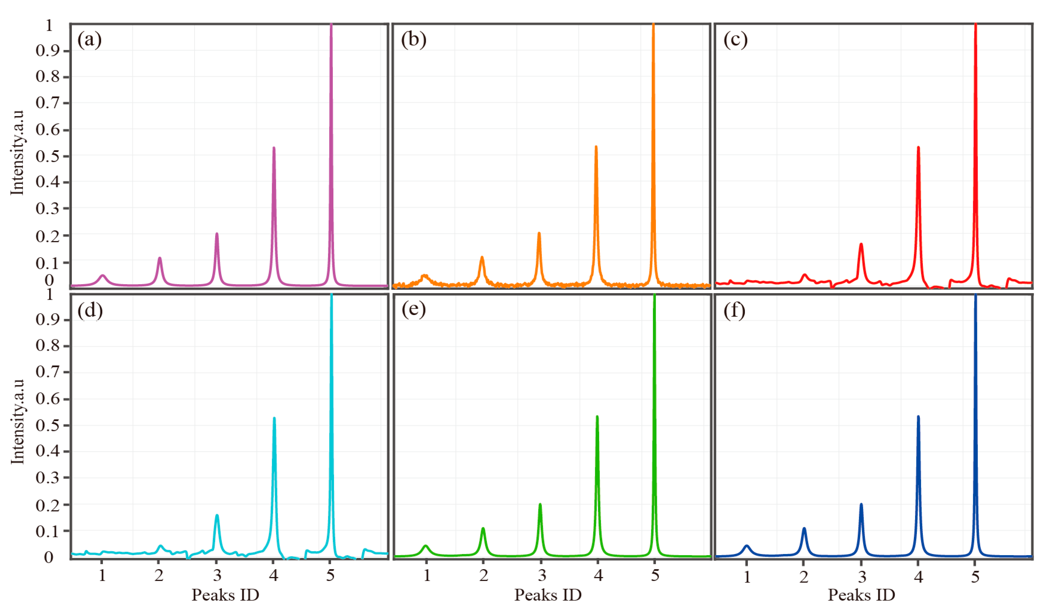
The synthetic 1D NMR spectrum is generated according to Equation (1), and its specific parameter settings are shown in

Table 3. Parameter settings of the synthetic 1D NMR spectrum.

	Peaks ID	1	2	3	4	5
Parameters
Amplitude ($A_j$)		0.3	0.4	0.5	1	1
Damping factor $({\tau }_j)$		0.01	0.02	0.03	0.04	0.08

. The total number of data points is 512, and 31 complex data points are acquired (means 6% NUS data). Then, simulated Gaussian noise with a mean of zero and a standard deviation of 0.005 is added to the FID. Here, the maximum value of the noise is lower than that of the lowest spectral peak.

The reconstruction results are shown in Figure 2. Under very limited sampled data, the first and second reconstructed spectral peaks are severely damaged in LRHM low-fidelity reconstructions, while the SLS and the proposed method reconstruct the spectral peaks with high fidelity (see the supplementary materials Table S1 for the correlation of each peak in Figure 2). In

Table 4. Statistics of peaks correlations and standard deviations.

	Peak ID	1	2	3	4	5
Method
LRHM		0.597 ± 0.384	0.859 ± 0.203	0.944 ± 0.090	0.991 ± 0.012	0.997 ± 0.004
LRHMF		0.600 ± 0.384	0.857 ± 0.203	0.943 ± 0.090	0.991 ± 0.012	0.997 ± 0.004
SLS		0.935 ± 0.183	0.974 ± 0.152	0.992 ± 0.039	0.999 ± 0.003	0.999 ± 0.001
SLSMF		0.936 ± 0.181	0.974 ± 0.152	0.993 ± 0.035	0.999 ± 0.002	0.999 ± 0.001

Note: Peak intensity correlations and error bars for the reconstructed spectra when 6% of data are acquired. The error bars are the standard deviations of correlations over 100 sampling trials. The numerical form of the table is $C\pm D$, where C is the mean of correlation, and D is the standard deviation.

, it is clearly shown that the robustness of the proposed method is consistent with SLS, and the Pearson correlation coefficient is much higher than LRHM at low intensity spectral peaks. The proposed method can accelerate the reconstruction of the best method, SLS, without compromising the spectra quality. Thus, it is correct and with the expectation that no significant difference between Figure 2f, the reconstructed spectra using SLSMF, and Figure 2e, the reconstructed spectra using SLS. Accordingly, LRHMF only accelerates the algorithm of LRHM, thus Figure 2c,d should be the same. In addition, in the supplementary materials, we displayed more reconstruction results of traditional methods with moderate-fidelity (Figure S2) and high-fidelity (Figure S3) from 100 simulation data trails and the correlation of their corresponding spectral peaks. Since the 1D reconstruction is fast (several seconds) for all compared methods, there is no need to compare the computation time.

4.2. Reconstruction of 2D NMR Spectra

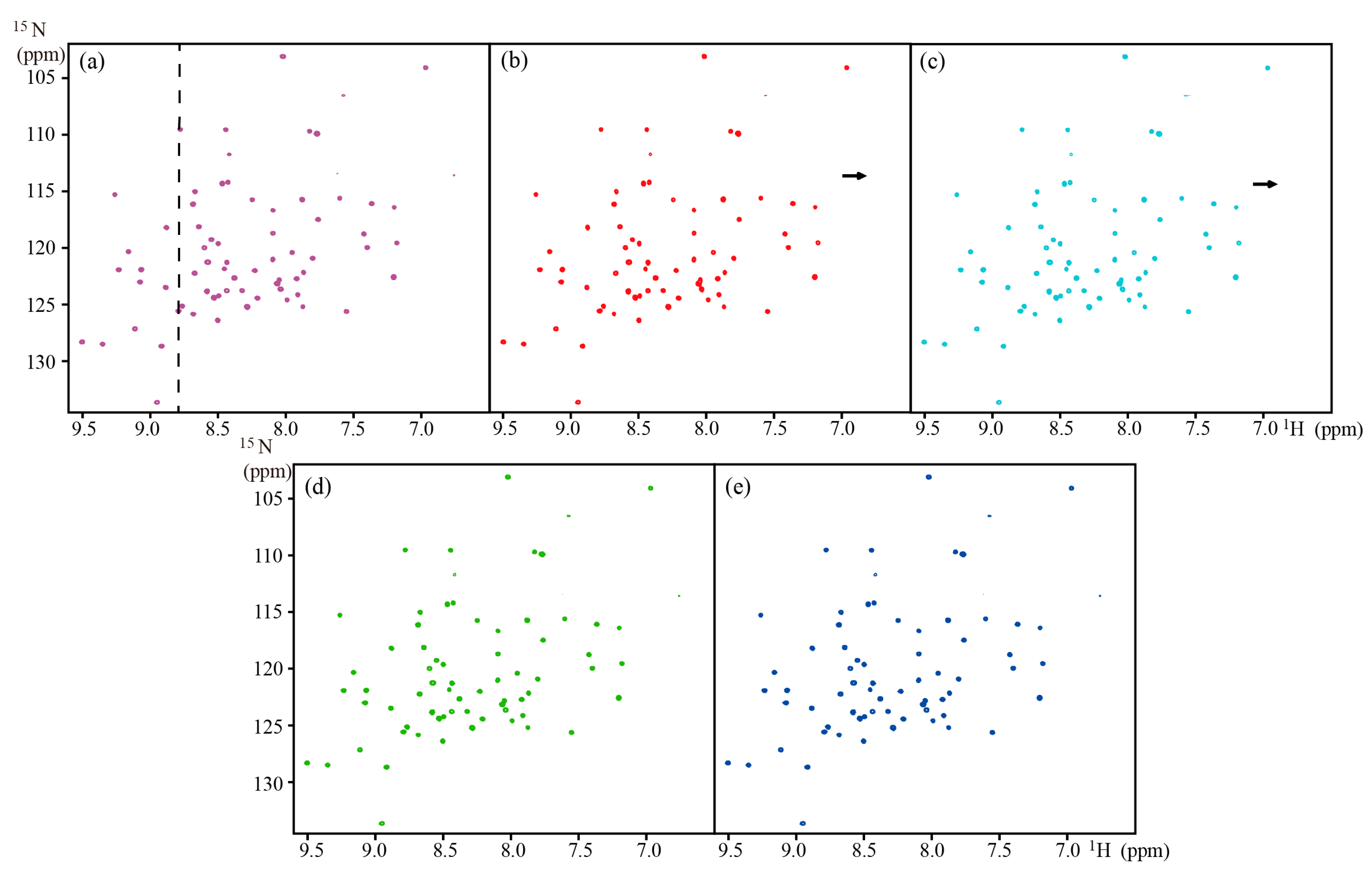
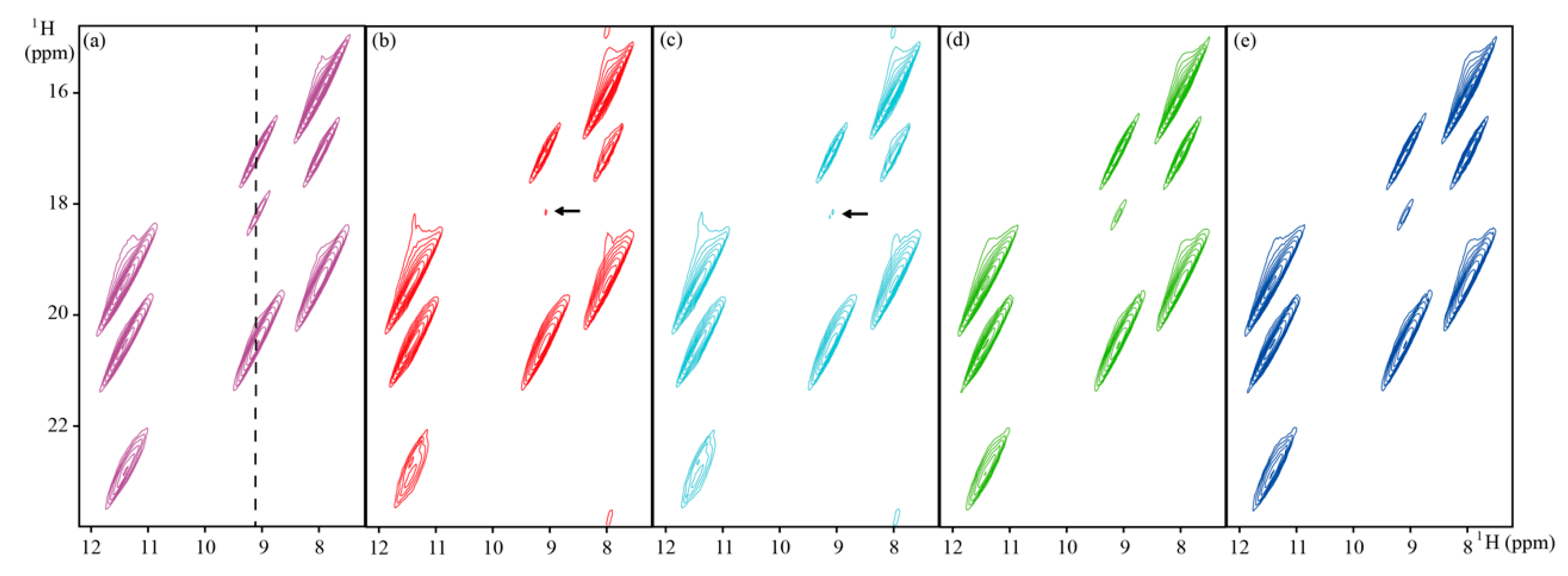
Reconstruction experiments with realistic NMR are conducted on 15% NUS 2D ¹H-¹⁵N HSQC spectra of GB1, 20% NUS 2D ¹H-¹⁵N best-TROSY spectra of ubiquitin, and 15% NUS 2D ¹H-¹H solid-state spectra.

Figure 3a, Figure 4a, and Figure 5a are fully sampled 2D ¹H-¹⁵N HSQC spectra of GB1, 2D ¹H-¹⁵N best-TROSY spectra of ubiquitin, and 2D ¹H-¹H solid-state spectrum, respectively. Results show that all methods can reconstruct a majority of spectral peaks well. However, some peaks in best-TROSY experiments shown by arrows in Figure 4b,c are lost in LRHM and LRHMF. LRHM and LRHMF also produce some pseudo peaks in the reconstructed GB1 and solid spectra, as shown by arrows in Figure 3b,c and Figure 5b,c. By contrast, SLS and SLSMF methods provide faithful reconstructions.

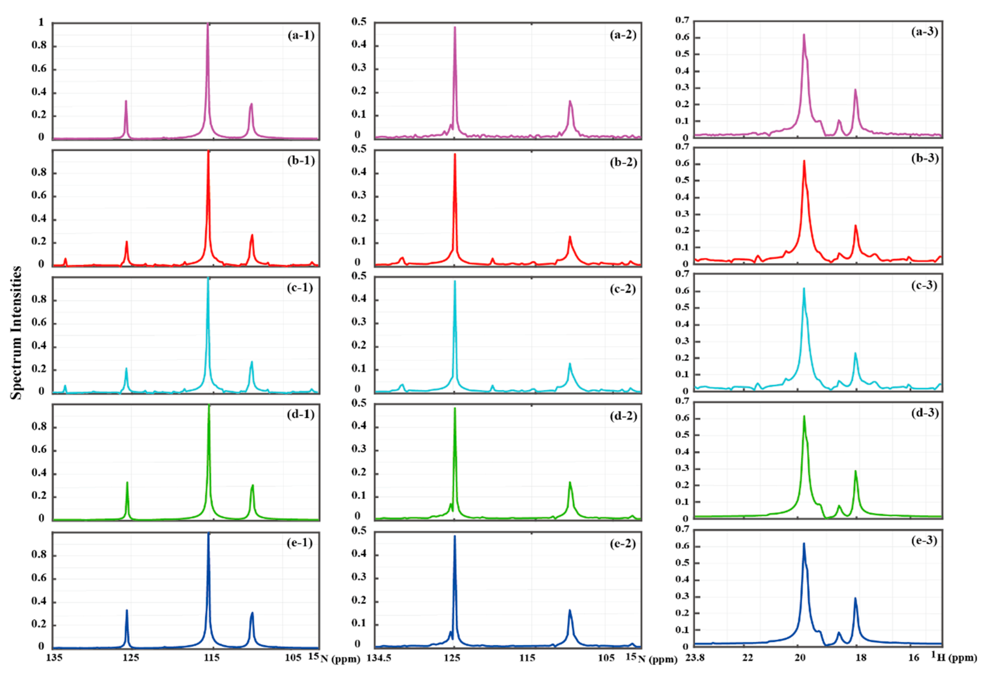
What is more, Figure 6 illustrates that the proposed method performs better in reconstructing low-intensity peaks. For example, LRHM and LRHMF weaken the reconstructed spectral peak near 125 ppm (Figure 6b–1,c–1) ), while SLSMF obtains the spectrum with peak intensity and line shape close to the fully sampled spectrum (Figure 6e–1).

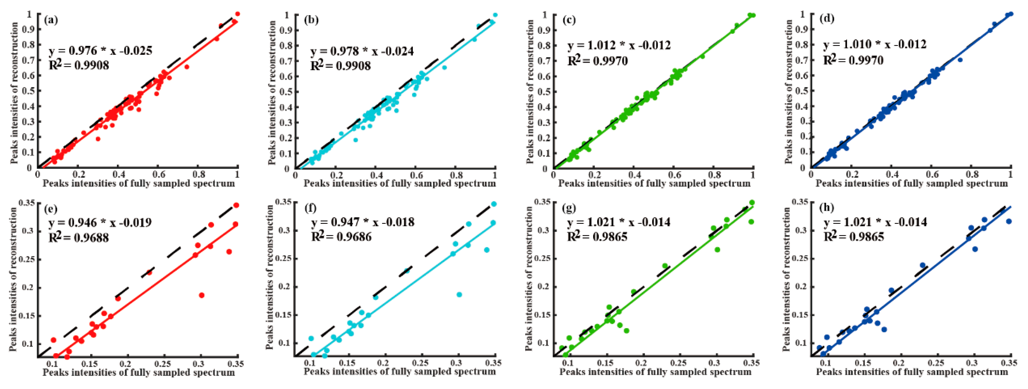
Regression analyses (Figure 7, Figure 8 and Figure 9) also exhibit that the SLSMF outperforms LRHM and LRHMF. It is shown that the SLSMF method gets a higher correlation than LRHM and LRHMF, especially in low-intensity peaks (Figure 7e–h, Figure 8e–h, and Figure 9e–h). Besides, lower RLNEsby SLSMF can be achieved than in LRHM and LRHMF, and RLNEs of SLSMF decrease much faster (Figure 10). For instance, we can see that after the update of the subspace, the RLNEs of SLSMF drop almost linearly, implying that the introduction of the signal subspace can help reconstruct high-fidelity spectra more quickly and accurately with the same sampling rate. The above observations indicate that in terms of reconstruction time and reconstruction quality, the proposed approach permits considerable improvements from the SLS and low-rank Hankel matrix methods.

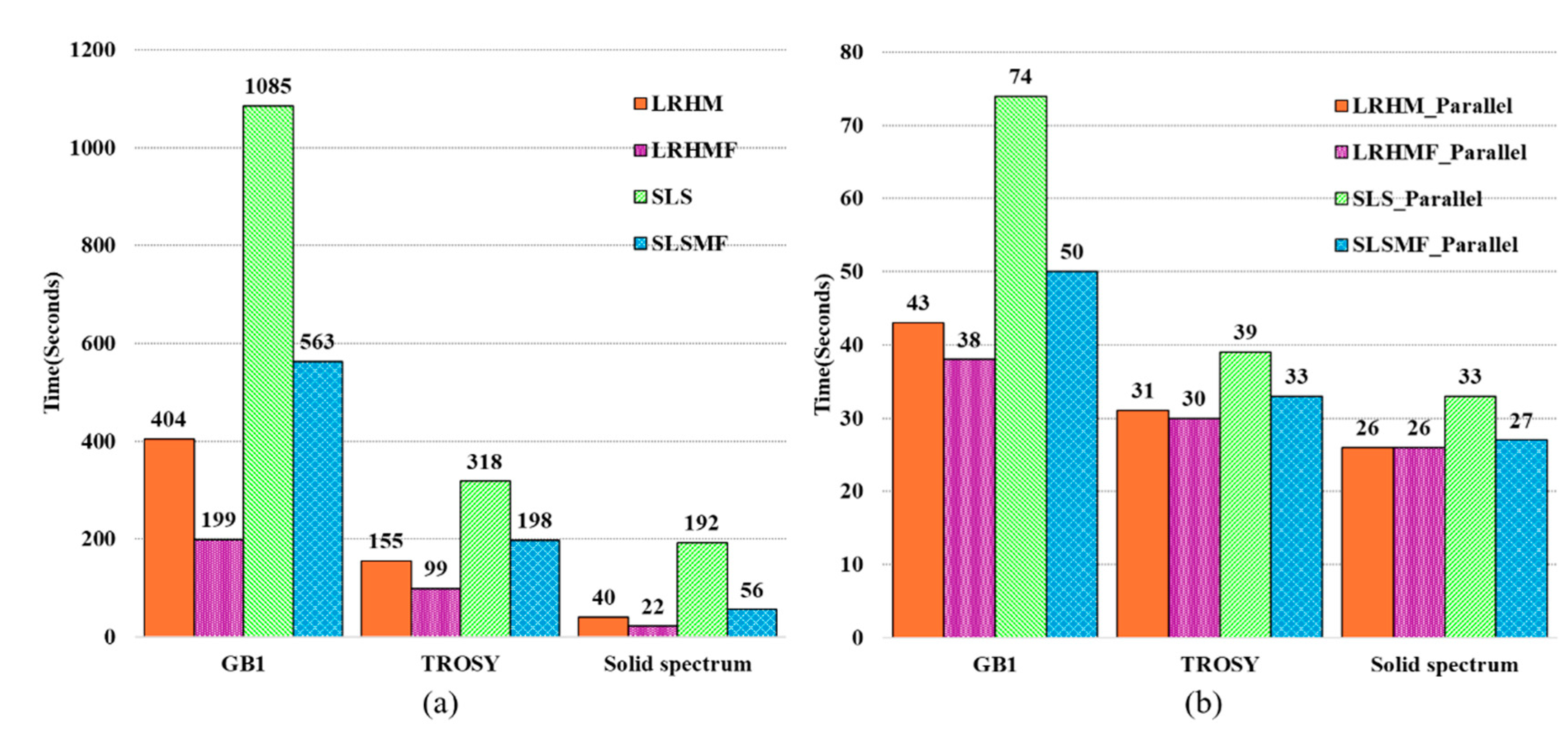
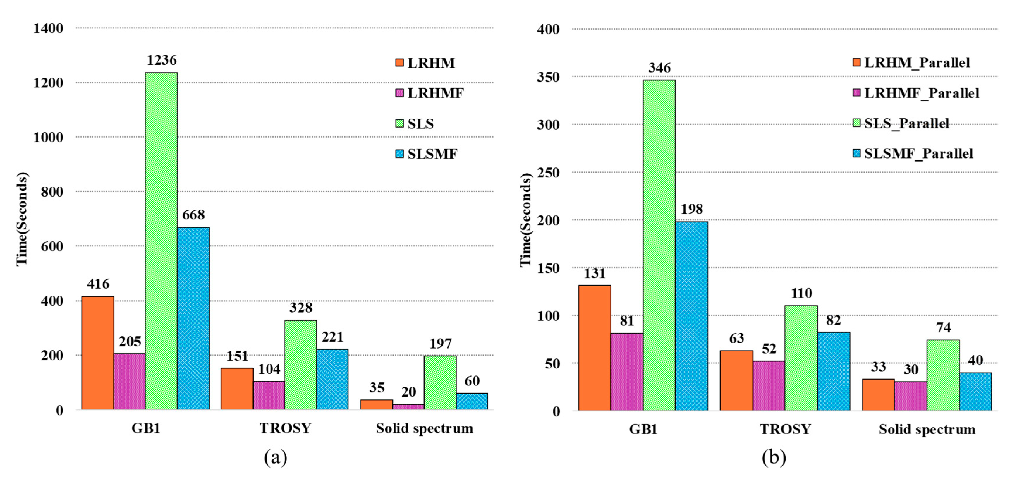
From Figure 11, we can see that compared to the SLS approach, the proposed method significantly speeds up the reconstruction time about 2–4 times (Figure 11a). If equipped with parallel computing architecture, the acceleration in the reconstruction time of SLSMF would be striking. Take the GB1 experiment as an example: With the parallel computing SLSMF, the time spent on reconstructing spectra only requires 4.6% of the computation of the SLS without parallelism. However, if the data dimension is too small, parallel computing is not recommended because it must pay for a certain time on switching the parallel pool, i.e., a mechanism used to control multiple processing cores in software. For example, for the reconstruction of the solid-state spectra, using the LRHMF only takes about 22 s, but it takes 26 s under parallel computing, whereas switching the parallel pool spends about 24 s. We also ran methods on the personal computer and the computation time, as reported in Figure 12. The calculation time with the personal computer also confirms that the proposed method can accelerate the reconstruction and can further reduce the time by parallel computing.

In the fast NUS NMR, high-fidelity reconstruction of the spectrum is most important, followed by the rest of other performances, such as the computation time. Our work is to design a new algorithm to reduce the computation time while achieving the best spectra. To emphasize our proposed method’s advantages in both reconstruction quality and speed, in

Table 5. Performance comparison of various methods.

	Quality	Peak Intensity Correlation		High-Fidelity Reconstruction Peaks	Reconstruction Time (Seconds)		Fast Reconstruction
Method		Low Intensity Peaks	All Peaks		Computing Server	Personal Computer
LRHM		0.9209	0.9826	No	116.5	138.2	No
LRHMF		0.9222	0.9870	No	69.0	82.0	Yes
SLS		0.9865	0.9979	Yes	290.2	381.8	No
SLSMF		0.9877	0.9979	Yes	154.5	211.5	Neutral

Note: R² denotes the square of the Pearson correlation coefficient. The correlation of low-intensity peaks and all peaks are averaged on all spectra in Figure 7, Figure 8 and Figure 9. The reconstruction time are averaged on all spectra in Figure 11 and Figure 12. The Pearson correlation coefficients of low-intensity peaks and all peaks are greater than 0.95 and 0.99, respectively, indicating high-fidelity reconstruction.

we list the advantages and disadvantages of the comparison method.

5. Conclusions

In this paper, a self-learning subspace matrix factorization (SLSMF) method is introduced to speed up the faithful reconstruction of highly-accelerated NMR spectroscopy. Comparisons with the state-of-the-art self-learning subspace method and the low-rank method imply that the new approach remarkably reduces computation time without sacrificing spectrum quality.

References

- Cavalli, A.; Salvatella, X.; Dobson, C.M.; Vendruscolo, M. Protein structure determination from NMR chemical shifts. Proc. Natl. Acad. Sci. USA 2007, 104, 9615–9620. [Google Scholar] [CrossRef] [Green Version]
- Tkáč, I.; Öz, G.; Adriany, G.; Uğurbil, K.; Gruetter, R. In vivo 1H NMR spectroscopy of the human brain at high magnetic fields: Metabolite quantification at 4t vs. 7t. Magn. Reson. Med. 2009, 62, 868–879. [Google Scholar] [CrossRef] [Green Version]
- Besghini, D.; Mauri, M.; Simonutti, R. Time domain NMR in polymer science: From the laboratory to the industry. Appl. Sci. 2019, 9, 1801. [Google Scholar] [CrossRef] [Green Version]
- James, K. Understanding NMR Spectroscopy; Wiley: Hoboken, NJ, USA, 2005. [Google Scholar]
- Orekhov, V.Y.; Jaravine, V.A. Analysis of non-uniformly sampled spectra with multi-dimensional decomposition. Prog. Nucl. Magn. Reson. Spectrosc. 2011, 59, 271–292. [Google Scholar] [CrossRef]
- Lam, F.; Li, Y.; Guo, R.; Clifford, B.; Liang, Z.-P. Ultrafast magnetic resonance spectroscopic imaging using spice with learned subspaces. Magn. Reson. Med. 2020, 83, 377–390. [Google Scholar] [CrossRef] [Green Version]
- Barna, J.C.J.; Laue, E.D.; Mayger, M.R.; Skilling, J.; Worrall, S.J.P. Exponential sampling, an alternative method for sampling in two-dimensional NMR experiments. J. Magn. Reson. 1987, 73, 69–77. [Google Scholar] [CrossRef]
- Mobli, M.; Hoch, J.C. Nonuniform sampling and non-fourier signal processing methods in multidimensional NMR. Prog. Nucl. Magn. Reson. Spectrosc. 2014, 83, 21–41. [Google Scholar] [CrossRef] [PubMed] [Green Version]
- Hyberts, S.G.; Takeuchi, K.; Wagner, G. Poisson-gap sampling and forward maximum entropy reconstruction for enhancing the resolution and sensitivity of protein NMR data. J. Am. Chem. Soc. 2010, 132, 2145–2147. [Google Scholar] [CrossRef] [PubMed] [Green Version]
- Kazimierczuk, K.; Stanek, J.; Zawadzka-Kazimierczuk, A.; Koźmiński, W. Random sampling in multidimensional NMR spectroscopy. Prog. Nucl. Magn. Reson. Spectrosc. 2010, 57, 420–434. [Google Scholar] [CrossRef] [PubMed]
- Jiang, B.; Jiang, X.; Xiao, N.; Zhang, X.; Jiang, L.; Mao, X.; Liu, M. Gridding and fast fourier transformation on non-uniformly sparse sampled multidimensional NMR data. J. Magn. Reson. 2010, 204, 165–168. [Google Scholar] [CrossRef]
- Petrellis, N. Undersampling in orthogonal frequency division multiplexing telecommunication systems. Appl. Sci. 2014, 4, 79–98. [Google Scholar] [CrossRef]
- Donoho, D.L. Compressed sensing. IEEE Trans. Inform. Theory 2006, 52, 1289–1306. [Google Scholar] [CrossRef]
- Qu, X.; Guo, D.; Cao, X.; Cai, S.; Chen, Z. Reconstruction of self-sparse 2D NMR spectra from undersampled data in the indirect dimension. Sensors 2011, 11, 8888–8909. [Google Scholar] [CrossRef] [PubMed] [Green Version]
- Ying, J.; Lu, H.; Wei, Q.; Cai, J.-F.; Guo, D.; Wu, J.; Chen, Z.; Qu, X. Hankel matrix nuclear norm regularized tensor completion for $ n $-dimensional exponential signals. IEEE Trans. Signal. Process. 2017, 65, 3702–3717. [Google Scholar] [CrossRef] [Green Version]
- Lu, H.; Zhang, X.; Qiu, T.; Yang, J.; Ying, J.; Guo, D.; Chen, Z.; Qu, X. Low rank enhanced matrix recovery of hybrid time and frequency data in fast magnetic resonance spectroscopy. IEEE Trans. Bio-Med. Eng. 2018, 65, 809–820. [Google Scholar] [CrossRef]
- Lam, F.; Liang, Z.-P. A subspace approach to high-resolution spectroscopic imaging. Magn. Reson. Med. 2014, 71, 1349–1357. [Google Scholar] [CrossRef] [Green Version]
- Kazimierczuk, K.; Orekhov, V.Y. Accelerated NMR spectroscopy by using compressed sensing. Angew. Chem. Int. Ed. Engl. 2011, 50, 5556–5559. [Google Scholar] [CrossRef]
- Holland, D.J.; Bostock, M.J.; Gladden, L.F.; Nietlispach, D. Fast multidimensional NMR spectroscopy using compressed sensing. Angew. Chem. Int. Ed. 2011, 50, 6548–6551. [Google Scholar] [CrossRef]
- Goowicz, D.; Kasprzak, P.; Kazimierczuk, K. Enhancing compression level for more efficient compressed sensing and other lessons from NMR spectroscopy. Sensors 2020, 20, 1325. [Google Scholar] [CrossRef] [Green Version]
- Qu, X.; Mayzel, M.; Cai, J.-F.; Chen, Z.; Orekhov, V. Accelerated NMR spectroscopy with low-rank reconstruction. Angew. Chem. Int. Ed. 2014, 54, 852–854. [Google Scholar] [CrossRef]
- Guo, D.; Qu, X. Improved reconstruction of low intensity magnetic resonance spectroscopy with weighted low rank Hankel matrix completion. IEEE Access 2018, 6, 4933–4940. [Google Scholar] [CrossRef]
- Hu, Y.; Zhang, D.; Ye, J.; Li, X.; He, X. Fast and accurate matrix completion via truncated nuclear norm regularization. IEEE Trans. Pattern Anal. 2013, 35, 2117–2130. [Google Scholar] [CrossRef] [PubMed]
- Guo, D.; Tu, Z.; Lu, H.; Qiu, T.; Xiao, M.; Qu, X. Reconstruction of Highly Accelerated NMR Spectra with Self-learning Subspace. Submitt. Anal. Chem. 2020. [Google Scholar]
- Jennings, A.; Mckeown, J.J. Matrix Computation; John Wiley & Sons: Hoboken, NJ, USA, 1992. [Google Scholar]
- Guo, D.; Lu, H.; Qu, X. A fast low rank Hankel matrix factorization reconstruction method for non-uniformly sampled magnetic resonance spectroscopy. IEEE Access 2017, 5, 16033–16039. [Google Scholar] [CrossRef]
- Zhang, X.; Guo, D.; Huang, Y.; Chen, Y.; Wang, L.; Huang, F.; Qu, X. Image reconstruction with low-rankness and self-consistency of k-space data in parallel MRI. Med. Image Anal. 2020, 63, 101687. [Google Scholar] [CrossRef] [Green Version]
- Hoch, J.C.; Stern, A.S. NMR Data Processing; Wiley-Liss: New York, NY, USA, 1996. [Google Scholar]
- Chen, D.; Wang, Z.; Guo, D.; Orekhov, V.; Qu, X. Review and prospect: Deep learning in nuclear magnetic resonance spectroscopy. Chem.-Eur. J. 2020. [Google Scholar] [CrossRef] [Green Version]
- Qu, X.; Huang, Y.; Lu, H.; Qiu, T.; Guo, D.; Agback, T.; Orekhov, V.; Chen, Z. Accelerated nuclear magnetic resonance spectroscopy with deep learning. Angew. Chem. Int. Ed. 2019. [Google Scholar] [CrossRef] [Green Version]
- Kazimierczuk, K.; Kasprzak, P. Modified omp algorithm for exponentially decaying signals. Sensors 2014, 15, 234–247. [Google Scholar] [CrossRef] [Green Version]
- Wan, S.; Mak, M.; Kung, S. Transductive learning for multi-label protein subchloroplast localization prediction. IEEE/ACM Trans. Comput. Biol. Bioinform. 2017, 14, 212–224. [Google Scholar] [CrossRef]
- Srebro, N. Learning with Matrix Factorizations; Massachusetts Institute of Technology: Cambridge, MA, USA, 2004. [Google Scholar]
- Signoretto, M.; Cevher, V.; Suykens, J.A.K. An SVD-free approach to a class of structured low rank matrix optimization problems with application to system identification. Organometallics 2013, 12, 4283–4285. [Google Scholar]
- Boyd, S.; Parikh, N.; Chu, E.; Peleato, B.; Eckstein, J. Distributed optimization and statistical learning via the alternating direction method of multipliers. Found. Trends Mach. Learn. 2011, 3, 1–122. [Google Scholar] [CrossRef]
- Vanessa, V.; Pablo, R.; Jean-Francois, M.; Raoul, V. NMR-Mpar: A fault-tolerance approach for multi-core and many-core processors. Appl. Sci. 2018, 8, 465. [Google Scholar]
- Mayzel, M.; Kazimierczuk, K.; Orekhov, V.Y. The causality principle in the reconstruction of sparse NMR spectra. Chem. Commun. 2014, 50, 8947–8950. [Google Scholar] [CrossRef] [PubMed] [Green Version]
Figure 1.
Schematic diagram of parallel computing of NMR spectroscopy reconstruction. Note: The blue dot represents the sampled data point and the white one represents unsampled data point; “Core j” represents the jth CPU (Central Processing Unit) core of a multi-core CPU for parallel computation. The non-uniform sampling (NUS) is performed along the indirect dimension (), and each 1D vector (in red rectangle) located at each data point in the direct dimension () can be reconstructed separately.
Figure 2.
Reconstructed synthetic 1D spectra with five peaks from 6% acquired data. (a) The fully sampled spectrum; (b) the noisy fully sampled spectrum; (c–f) reconstructed spectra using the low-rank Hankel matrix (LRHM), LRHM with matrix factorization (LRHMF), self-learning subspace (SLS) and SLSMF, respectively.
Figure 3.
Reconstructed 2D HSQC spectra of GB1 with 15% NUS data. (a) The fully sampled spectrum; (b–e) reconstructed spectra using the LRHM, LRHMF, SLS, and SLSMF, respectively. Note: The contours of spectra are at the same level.
Figure 4.
Reconstructed 2D 1H–15N best-TROSY spectra of ubiquitin with 20% NUS data. (a) The fully sampled spectrum; (b–e) reconstructed spectra using the LRHM, LRHMF, SLS, and SLSMF, respectively. Note: The contours of spectra are at the same level.
Figure 5.
Reconstructed solid NMR spectra with 15% NUS data. (a) The fully sampled spectrum; (b–e) reconstructed spectra using the LRHM, LRHMF, SLS, and SLSMF, respectively. Note: The contours of spectra are at the same level.
Figure 6.
1D traces of reconstructed 2D spectra (a-1)–(a-3) is the fully sampled spectrum of the 1D traces of HSQC spectra of GB1, the best-TROSY spectrum of ubiquitin, and solid NMR spectrum, respectively. (b-1)–(b-3), (c-1)–(c-3), (d-1)–(d-3), and (e-1)–(e-3) are reconstructed spectra using LRHM, LRHMF, SLS, and SLSMF, respectively. Note: (a-1)–(a-3) are fully sampled spectra of 1D traces, and their locations in the corresponding fully sampled spectrum are marked with a dotted line in Figure 3, Figure 4 and Figure 5.
Figure 7.
Peak intensity correlation between fully sampled spectrum and reconstructed spectra on the 2D HSQC of GB1. (a–d) are correlation plots of all peaks using LRHM, LRHMF, SLS, and SLSMF, respectively. (e–h) are correlation plots of low-intensity peaks using LRHM, SLS, and SLSMF, respectively.
Figure 8.
Peak intensity correlation between fully sampled spectrum and reconstructed spectra on the 2D 1H-15N best-TROSY spectrum of ubiquitin. (a–d) are correlation plots of all peaks using LRHM, LRHMF, SLS, and SLSMF, respectively. (e–h) are correlation plots of low-intensity peaks using LRHM, SLS, and SLSMF, respectively.
Figure 9.
Peak intensity correlation between fully sampled spectrum and reconstructed spectra of the solid NMR. (a–d) are correlation plots of all peaks using LRHM, LRHMF, SLS, and SLSMF, respectively. (e–h) are correlation plots of low-intensity peak using LRHM, SLS, and SLSMF, respectively.
Figure 10.
The RLNEs versus times of different approaches. (a–c) are the RLNE curves of the 1D experiments marked with a dotted line in Figure 3a, Figure 4a, and Figure 5a, respectively. Note: The point indicated by the arrow in the Figure is to update the outer subspace.
Figure 11.
The computation time of spectra reconstruction on a computational server using the LRHM, LRHMF, SLS, and SLSMF methods. (a,b) computation time of spectra reconstruction without and with parallel computing, respectively. Note: The switching on and off parallel pool takes an average of 24 s.
Figure 12.
The computation time of spectra reconstruction on a personal computer. (a,b) computation time of spectra reconstruction without and with parallel computing, respectively. Note: All reconstruction algorithms were performed using MATLAB 2017b (Mathworks Inc., Natick, MA, USA) on a personal computer with 1.80 GHz 4 cores CPU and 8 GB RAM. The switching on and off parallel pool takes an average of 24 s.