Motion Planning and Coordinated Control of Underwater Vehicle-Manipulator Systems with Inertial Delay Control and Fuzzy Compensator


1
College of Automation, Harbin Engineering University, Harbin 150001, China
2
College of Information and Communication Engineering, Harbin Engineering University, Harbin 150001, China
*
Author to whom correspondence should be addressed.
Appl. Sci. 2020, 10(11), 3944; https://doi.org/10.3390/app10113944
Submission received: 28 April 2020
/
Revised: 27 May 2020
/
Accepted: 29 May 2020
/
Published: 5 June 2020
(This article belongs to the Special Issue Modelling and Control of Mechatronic and Robotic Systems)
Abstract
:This paper presents new motion planning and robust coordinated control schemes for trajectory tracking of the underwater vehicle-manipulator system (UVMS) subjected to model uncertainties, time-varying external disturbances, payload and sensory noises. A redundancy resolution technique with a new secondary task and nonlinear function is proposed to generate trajectories for the vehicle and manipulator. In this way, the vehicle attitude and manipulator position are aligned in such a way that the interactive forces are reduced. To resist sensory measurement noises, an extended Kalman filter (EKF) is utilized to estimate the UVMS states. Using these estimates, a tracking controller based on feedback Linearization with both the joint-space and task-space tracking errors is proposed. Moreover, the inertial delay control (IDC) is incorporated in the proposed control scheme to estimate the lumped uncertainties and disturbances. In addition, a fuzzy compensator based on these estimates via IDC is introduced for reducing the undesired effects of perturbations. Trajectory tracking tasks on a five-degrees-of-freedom (5-DOF) underwater vehicle equipped with a 3-DOF manipulator are numerically simulated. The comparative results demonstrate the performance of the proposed controller in terms of tracking errors, energy consumption and robustness against uncertainties and disturbances.
1. Introduction
With increasing interest in the field of marine research, autonomous underwater vehicle manipulator systems (UVMSs) [1] have rapidly developed into important devices for exploring the ocean, completing underwater tasks, underwater sampling and so on. It is a challenging problem to accurately control the UVMS in an energy-efficient manner due to the kinematic redundancy and underwater environment with hydrodynamic uncertainties, unknown external disturbances (such as ocean currents) and inaccurate sensor information. For solving these problems, inverse kinematics and robust coordinated control techniques have been developed for the UVMS.
For the inverse kinematics of the UVMS, the solution can be obtained through mapping the end-effector’s velocities to the velocities of the vehicle and manipulator. As the UVMS has redundant degrees of freedom (DOFs), there are various combinations of vehicle and manipulator velocities without affecting the end-effector velocities. A common solution is to adopt the pseudo-inverse Jacobian matrix of the UVMS or its weighted form [2]. However, this method is not desirable for redundant exploration to avoid joint limits, improve system manipulability or save energy. Therefore, the task-priority redundancy resolution technique [3] was proposed in such a way that the fulfillment of the primary task has a higher priority than that of a secondary task. Generally, the secondary task is to optimize the performance index through assigning additional motion in the null space of the primary task. Sarkar and Podder [4] solved the inverse kinematics of the UVMS on the acceleration level to minimize the total hydrodynamic drag; however, the performance index of this method requires dynamic equations which can not be modeled exactly. Han et al. [5] proposed a new performance index designed to minimize restoring moments without using dynamic equations. However, this method was implemented for a specific configuration of the UVMS.
The task-priority strategy can be extensible to chain multiple tasks which have a lower order of priority (Siciliano and Slotine [6]). Antonelli et al. [7] used a fuzzy inference system (FIS) to handle multiple secondary tasks, such as reduction of fuel consumption and improvement of system manipulability. In such a way, a secondary task can be activated by FIS when the corresponding variable is without the safe range. Wang et al. [8] used a fuzzy logic algorithm to decide the priorities of secondary objectives, such as manipulator singularity avoidance and attitude optimization of the UVMS. The experimental validation of three difference kinematic control schemes was presented in [9]. In [10], a multitask kinematic control of the underwater biomimetic vehicle-manipulator system (UBVMS) was designed. A unifying framework for the kinematic control of UVMSs was proposed in [11]. A very recent work dedicated to motion planning for the UVMS was presented in [12].
To achieve trajectory tracking, it is very important to design a coordinated motion controller for the UVMS. The simple control methods (e.g., proportional-integral-derivative (PID) control) are not suitable for the UVMS due to the inherent nonlinear and coupled dynamics of the system [13,14,15]. Schjlberg and Fossen [16] proposed a control strategy in terms of feedback linearization. Sarkar and Podder [4] utilized a computed torque controller (CTC) for trajectory tracking of the UVMS. Taira et al. [17] proposed a model-based motion control for the UVMS, which can be applicable to three types of servo systems; i.e., a voltage-controlled, a torque-controlled and a velocity-controlled servo system. Korkmaz et al. [18] presented a trajectory tracking control for an underactuated underwater vehicle manipulator system (U-UVMS) based on the inverse dynamics. However, these model-based controllers are poor in terms of robustness against model uncertainties. In [19], a fuzzy logic control method was designed for a hybrid-driven UVMS to grasp marine products on the seabed. A model reference adaptive control approach for an UVMS was proposed in [20]. Antonelli et al. [21] proposed an adaptive controller based on virtual decomposition; however, a regressor matrix corresponding to parameter vector is required in this method. An indirect adaptive controller based on the extended Kalman filter (EKF) was proposed in [22]; meanwhile the performance would be degraded due to the estimated error via EKF. To eliminate the bias from the EKF estimation, Dai et al. [23] introduced a H∞ control in the indirect adaptive controller to achieve robust performance. However, this method results in a residual error when the bounds of the disturbance cannot be known prior. To reduce or omit the estimation error of the uncertainties and disturbances, a fuzzy compensator based on estimations was utilized [24]. To handle state and input constraints of the UVMS, a robust predictive control (RMPC) [24], a nonlinear MPC (NMPC) [25], a tube-based robust MPC [26], a fast MPC (FMPC) [27] and a fast tube MPC (FTMPC) [28] were used for the UVMS trajectory tracking, but these MPC approaches do not permit the self-motion utilized to perform energy efficient trajectory tracking.
For achieving precise and robust performance, the control design should be enhanced by the estimations of the system’s uncertainties and disturbances. The popular estimation techniques include time delay control (TDC) [29,30], the extended state observer (ESO) [31], the disturbance observer [32], the nonlinear disturbance observer (NDO) [33,34] the uncertainty and disturbance estimator (UDE) [35,36] (redefined as inertial delay control (IDC) [37]) and so on. Among them, because IDC is simple in design and easy to complete, it is widely used to estimate the effect of the lumped uncertainties and disturbances. Generally, the IDC is applied to the sliding mode control (SMC) for ensuring precise and robust performance. The combined method does not require the bounds of uncertainties and disturbances, and it does not use the discontinuous function in the control law.
However, the above-mentioned methods are based on joint-space variables, which may not be suitable for a variety of underwater tasks with high-precision end-effector position requirements [38]. These task space control schemes can easily adapt to the online modification of the end-effector’s motion [39,40]. However, the task-space controllers also have disadvantages. (a) The kinematic redundancy of the UVMS cannot be exploited. (b) The output of the task-space controller should be mapped into the joint space so as to be realized by thrusters and actuators. Li et al. [34] proposed a hybrid strategy-based coordinated controller for the UVMS. The hybrid strategy is to transform the joint-space controller (to exploit the system’s redundancy) to the task-space controller (to ensure high-accuracy tracking performance).
Inspired by the above studies, new motion planning and coordinated control schemes of the UVMS are proposed in this paper. The contribution of this work is that the proposed scheme can ensure precise, energy-efficient and robust performance in the presence of model uncertainties, external disturbances, payload and sensory noises. First, a new redundancy resolution technique is proposed, where a new secondary task with a nonlinear function is inserted for generating energy-saving trajectories for the vehicle and manipulator. Second, an EKF estimation system is employed for resisting sensory noises. Third, a coordinated motion control with joint-space errors, end-effector errors, IDC and a fuzzy compensator is proposed as a robust tracking controller against uncertainties and disturbances. Last, the effectiveness of the proposed scheme is verified through numerical simulations.
The rest of the paper is organized as follows. Section 2 is concerned with the kinematic and dynamic modeling of the UVMS. In Section 3, an improved redundancy resolution technique is presented. The proposed control scheme is proposed in Section 4. Numerical simulations and the detailed performance analysis are presented in Section 5. Section 6 holds the conclusions.
2. Modeling
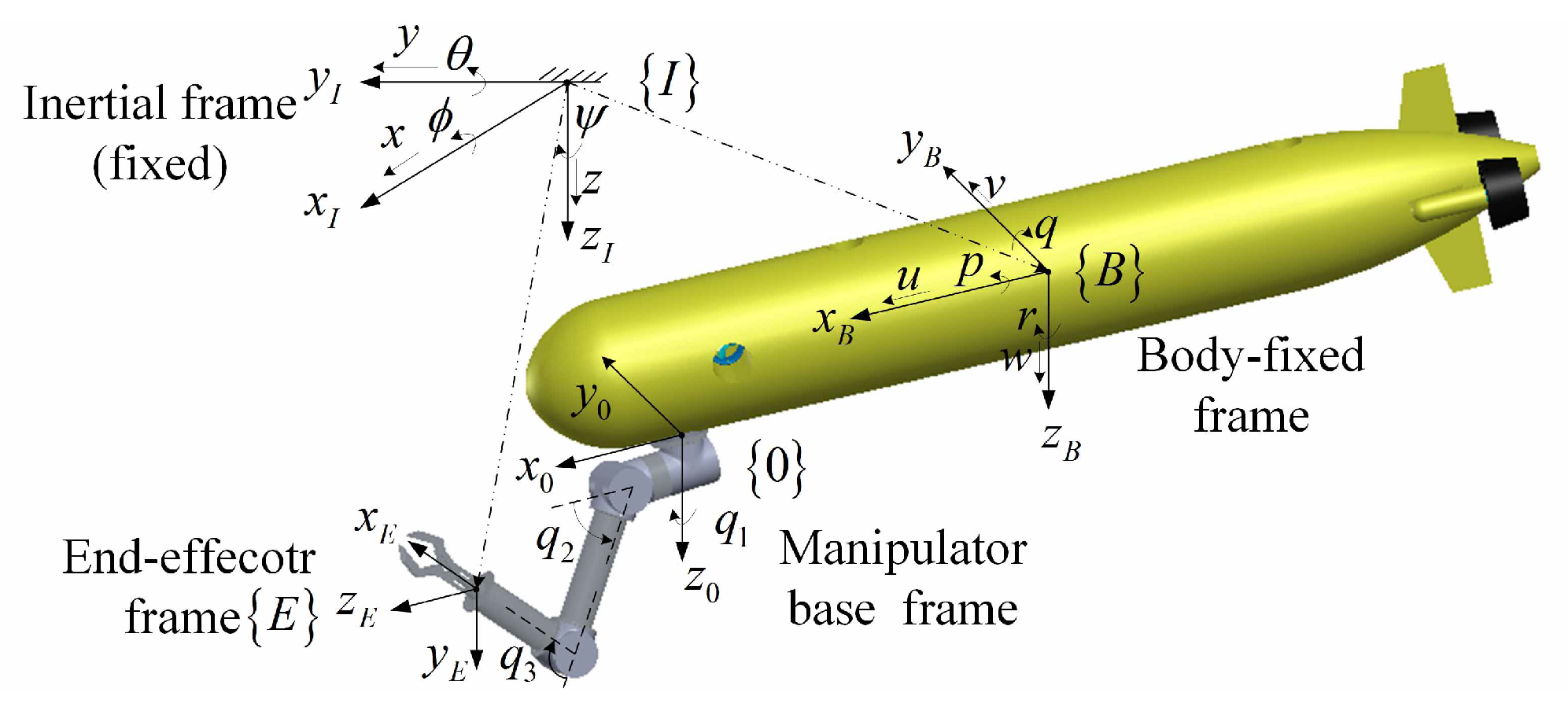
The UVMS investigated in this paper is composed of an underwater vehicle with a 3 DOFs manipulator. The coordinate system of the UVMS is shown in Figure 1. In the body-fixed frame , we define that the vectors of vehicle’s linear and angular velocities are and , where , and . The vector of joint positions is assumed to be , where n is the number of manipulator’s joints. The position and orientation vector of the UVMS relative to the body-fixed frame is assumed to be . In the inertial frame , the vectors of end-effector’s position and orientation are defined as and , and assume .
The kinematic model of the UVMS [21] can be obtained as shown in (1), where the velocities of the UVMS in the body-fixed frame () are mapped into end-effector velocities () via .
where , , and . is the rotational matrix describing the transformation from the manipulator’s base frame to the body-fixed frame, and is the position vector from manipulator’s base to the center of the body-fixed frame. is the position vector from end-effector to the manipulator’s base. is the manipulator’s linear Jacobian matrix, and is the manipulator’s angular Jacobian matrix. is the cross-product operator.
The vectors of vehicle’s position and attitude relative to the inertial frame are defined as and , where , and . The velocity vector of the UVMS defined in the body-fixed frame () can be obtained by (2).
where , and . is the linear rotational matrix describing the transformation from the inertial frame to the body-fixed frame, and is the angular rotational matrix. The values of and can be referred to the literature [41]. is the Jacobian matrix which relates the vehicle velocities with respect to the inertial frame and the body-fixed frame.
Dynamic Modeling
The nonlinear dynamic equations of the UVMS expressed in the body-fixed frame can be established as [16,21]:
where
where is the inertia matrix including added mass terms, and and are matrices of the inertia effects due to the manipulator. is the Coriolis and centripetal matrix, and (i = 1,3)/ is the matrix of Coriolis and centripetal forces due to the coupling effects/due to the manipulator. is the vector of dissipative effects, and is the matrix of drag effects due to the coupling effects. is the vector of gravity and buoyancy effects, is the restoring vector of the vehicle, is the restoring vector of the manipulator and is the restoring vector due to the manipulator. is the vector of generalized forces. is the vector of disturbances. Generally, in a deep water environment, comes from ocean currents, payload, etc. In particular, time-varying ocean currents increase the uncertainty of the UVMS hydrodynamic forces, making accurate control of the UVMS difficult.
As for the underwater manipulator, it is assumed that its links are composed of cylindrical elements. The hydrodynamic effects on cylinders can be referred to [16]. For a cylinder, the inertial matrix of added mass and added moment is a diagonal matrix, while the off-diagonal elements are neglected. The drag force can be expressed by a nonlinear function related to the velocity vector of the center of mass of the link. Generally, when calculating the hydrodynamic forces, the linear skin-friction force, quadratic drag force and lift force are considered. The third-order and higher order terms of the drag forces are neglected. In addition, based on the assumption that velocity of the ocean current is constant, the diffraction forces can be neglected.
In the real system, the above model parameters are usually difficult to accurately measure or estimate, especially the hydrodynamic forces acting on the UVMS. Thus, it is advisable to divide the model parameters into two parts: the normal value part and the bias part. The normal value is denoted as , which can be obtained through using strip theory, pool experiment analysis or CFD computation. The bias term is denoted as Δ(·), which describes the difference between the real value and the nominal value. Then, (4) can be obtained. For control design, the normal values are available, while the bias parts are considered as model parameter uncertainties.
Considering that the vehicle is driven by thrusters and the manipulator is driven by motors, the generalized force vector is related to the vector of thruster forces and actuator torques through (5).
where . represents the vector of thruster forces, and represents the vector of actuator torques. is the thruster configuration matrix, and is the thruster-actuator configuration matrix. It is known that for an under-actuated underwater vehicle, . Generally, for a manipulator, n joint motors are all available.
3. Proposed Redundancy Resolution
This section proposes a new redundancy resolution technique to generate energy-efficient trajectories for the vehicle and the manipulator. It is known that infinite solutions of the UVMS inverse kinematics can be obtained by inverting the mapping (1). The solution using the pseudo inverse of the Jacobian matrix is expressed as [2]
where is the end-effector velocity vector. is the pseudo inverse of the Jacobian matrix and .
However, this solution does not exploit the redundant DOFs of the system, and it is not suitable from the perspective of energy consumption. Therefore, a new task-priority redundancy resolution technique is proposed in this section. In the proposed technique, the primary task is to map the end-effector variables into the joint-space variables, and two secondary tasks are provided to explore the kinematic redundancy for energy savings, joint limit avoidance and small roll and pitch angles kept for the vehicle, as shown in (7).
where is the weighted pseudo-inverse Jacobian matrix. is considered as the primary task Jacobian matrix and is the motion distribution matrix with elements belonging to . When the diagonal elements of the former three rows of are close to 1, the diagonal elements of the later n rows of will be close to 0. This results in greater movement of the vehicle and less movement of the manipulator. Otherwise, when the diagonal elements of the former three rows of are close to 0, the diagonal elements of the later n rows of will be close to 1. This results in less movement of the vehicle and greater movement of the manipulator. The diagonal elements of the middle three rows of correspond to the movement of the vehicle’s attitude. The larger they are, the greater the movement of the vehicle’s attitude. The off-diagonal elements of describe the degrees of the coupling effects between the DOFs of the UVMS, which can refer to our previous work [15]. The closer the off-diagonal element of to 1, the greater the corresponding coupling motion. and are the secondary task Jacobian matrices. It can be recognized that the secondary tasks are fulfilled in the null space, which will not affect the motion of the primary task. Moreover, the two secondary tasks have the same lower priority relative to the primary task. is the primary-task vector and is the error of the primary task. is a secondary-task vector to achieve system coordination between its rotational subsystem and translational subsystem, including the vehicle attitudes and joint angles, and is its error. and are positive definite matrices. The other secondary task vector is the velocity vector of the UVMS , which contributes to the system’s self-motion utilized for reducing energy requirements. is a diagonal matrix whose elements belong to . The larger the diagonal element of , the greater the corresponding coupling motion. For instance, if the diagonal element of the secondary row of is larger, the vehicle will have a larger yaw angle according to the coupling effects. Similarly, if the diagonal element of the third row of is larger, the vehicle will have a larger pitch angle. is a coefficient belonging to , which is used to adjust the values of .
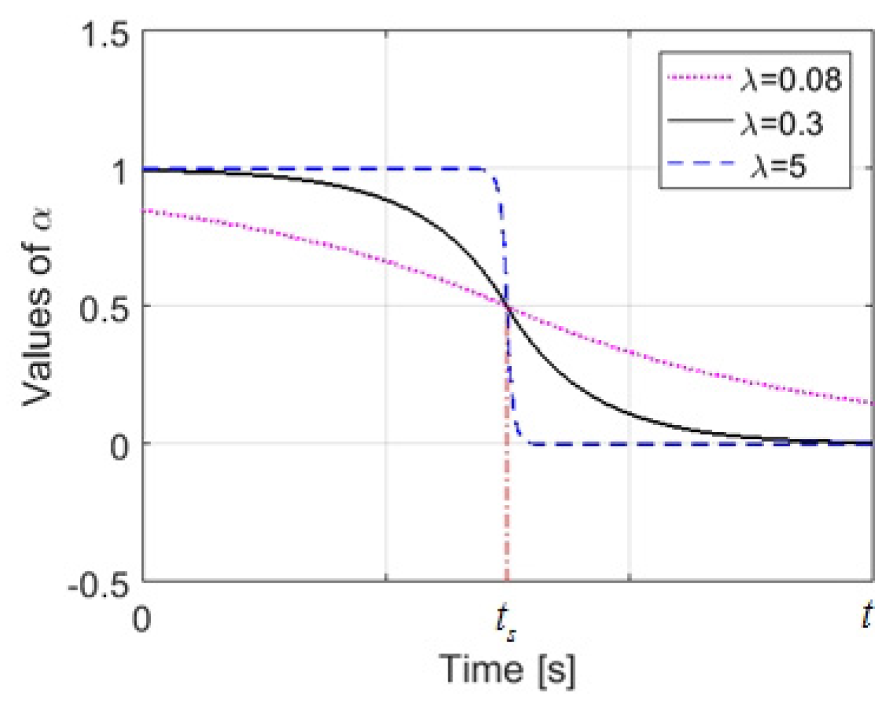
To effectively utilize the self-motion during the entire UVMS motion, is defined as a nonlinear function related to time , as given in (8).
where relatives to the time at which the system enters deceleration phase. is the coefficient and .
The curve of the nonlinear function is shown in Figure 2. It can be recognized that the smaller the value of , the smoother the variations of the nonlinear function. Therefore, it is better to choose a small value of to ensure smooth movement of the UVMS.
4. Control Design
The purpose of control design is to obtain the values of thruster forces and actuator torques in order to drive the UVMS to the desired trajectory. In addition, the robustness of the designed controller is important in the presence of model parameter uncertainties, time-varying external disturbances, payload variations and sensory noises. In this section, for precise and robust control of the UVMS, a new coordinated motion controller including inertial delay control (IDC) and a fuzzy compensator is proposed. Besides, the proposed controller uses the estimated UVMS states via an EKF.
4.1. Design of an EKF
Due to the presence of sensory measurement noises, the vehicle and manipulator positions measured by sensors are not inaccurate. Therefore, it is necessary to utilize a nonlinear filter to estimate the system’s states. As the extended Kalman filter (EKF) is simple and easy to complete and has low computational complexity, the EKF is used in this study. It is necessary to obtain a linear model during the KF design process. The dynamic equations of the UVMS can be linearized by ignoring the higher order terms in the expended Taylor series. The state vector of the system, e.g., position/attitude and velocity vectors, is defined as . The measurement model can be expressed as .
Based on (2) and (3), the time derivative of the system state vector can be obtained as
where is considered as the estimated model of the system.
With the additive Gaussian white noise, the predicted system state vector at is given in (10), and the predicted measurement state vector at is shown in (11). Then the covariance matrix of the predicted state vector can be obtained as shown in (12).
where is the predicted state vector at . is the vector of system noises. is the vector of measurement noises. is the covariance matrix of the estimated system states.
Therefore, the estimated system states can be obtained through the following correction step:
where and
4.2. Design of a Tracking Controller
The control objective is to make sure that the tracking errors quickly converge to zero under the conditions of model parameter uncertainties, time-varying external disturbances and payload. First, the tracking errors of the system are defined. The vector of end-effector tracking errors is shown in (16), and the vectors of tracking errors in the joint space are shown in (17)–(19).
where the superscript denotes the corresponding estimated values via EKF, and the subscript denotes the corresponding desired values. and are the quaternions of and .
Then, the tracking controller based on feedback linearization is given as
where is the Jacobian matrix of the system, as given in (1). , and are the positive symmetric matrices. is the estimated vector of the lumped uncertainties and disturbances, which is described in the next subsection.
4.3. Inertial Delay Control (IDC)
Due to the underwater circumstances, the dynamic equations of the UVMS include unknown external disturbances and an amount of parameter uncertainties caused by identification errors. These lumped uncertainties and disturbances can be expressed as (21) with reference to (3) and (4).
where and denote the estimates of the system states via EKF.
Substituting the proposed control law (20) in (22), dynamical equation of the tracking errors is
where is the estimated error vector.
It is assumed that a slow-varying signal can be approximated and estimated by a filter with appropriate bandwidth [37]. Based on this assumption, the uncertainty and disturbance estimator (UDE) is proposed for estimating slow-varying uncertainties [35,37]. Then, the estimations of lumped uncertainties and disturbances can be given as
where is a strictly proper low-pass filter possessing a uniform steady-state gain and a sufficiently large bandwidth. Based on (24), it is found that by passing the lumped uncertainties and disturbances through a inertial filter , the estimation vector can be obtained. The UDE method is redefined as inertial delay control (IDC) [37], because it is analogous to the time delay control (TDC) which delays the plant signals in time to obtain the estimates.
A choice of with first order is given by
where is a diagonal matrix with small positive constant. is the identity matrix.
Then (25) can be rewritten as
Therefore, the estimates of the lumped uncertainties and disturbances can be obtained as
If the lumped uncertainties and disturbances are slowly varying, then is small and . Therefore, the estimated errors () go to zero asymptotically. If is not small, but is small, is ultimately bounded and the estimated accuracy can be improved by estimating and .
4.4. Fuzzy Compensator
Based on the estimates via IDC, the fuzzy compensator is given as
where is the parameter of the fuzzy compensator, and is a constant vector.
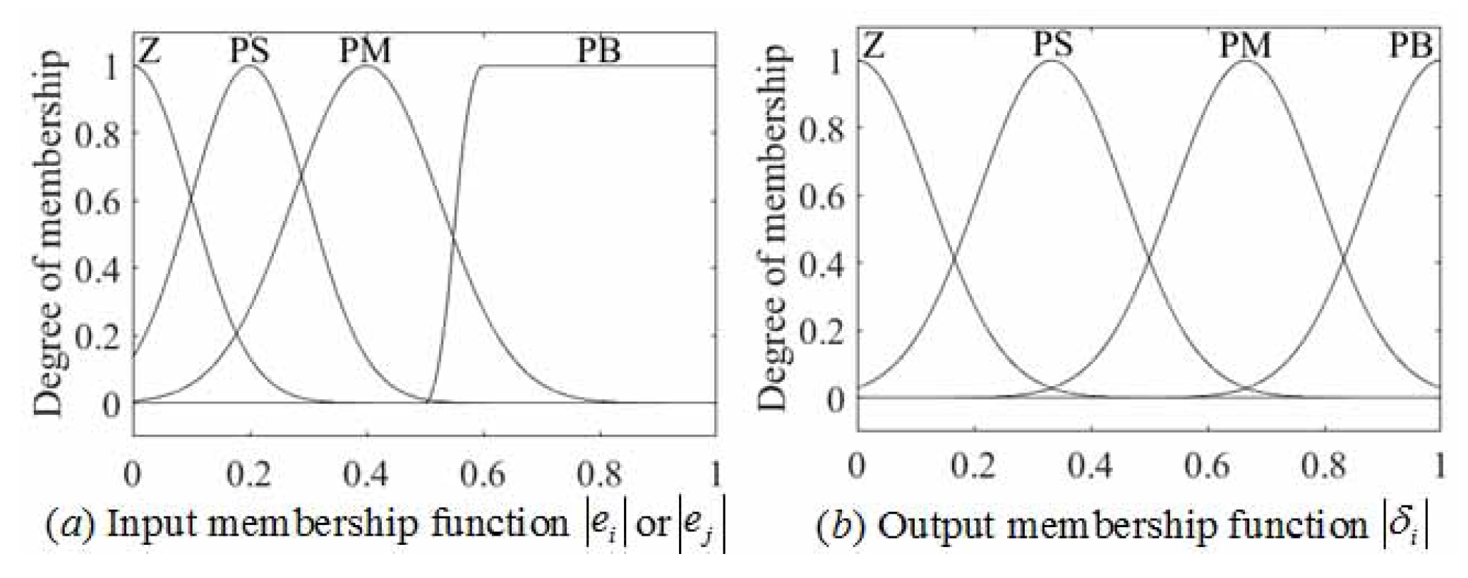
The fuzzy compensator is a multiple-inputs-single-output fuzzy logic controller (FLC) with the joint-space system errors and as two input variables and after defuzzification and denormalization as an output variable. Denote the system error vector (as given in (17)) as . The main advantage of this fuzzy compensator is that the required fuzzy rules take the dynamic coupling between the vehicle and the manipulator [15,16] into account. It is known that the roll, pitch and yaw motions of the vehicle are coupled with its surge, sway and heave motions. As the roll and pitch angles should be kept small for properly working of the bottom sensors, it is assumed that the surge and sway motions are mostly affected by the yaw angle. Note that the pitch and heave motions are interactive, and the manipulator’s joints 2 and 3 are interactive. The position of manipulator’s joint 1 is mostly affected by the sway motion. Based on these analysis, the fuzzy rules are given in Table 1. Table 2 shows the relationships between an output and two input variables.
The following symbols are used in Table 1: ZE (zeros), PS (positive small), PM (positive medium), PB (positive big). Figure 3a,b shows the member functions of the normalized input and output variables respectively. After the fuzzification stage, the Mamdani inference method is used for fuzzy implication, and then the centroid method is used for defuzzification. Finally, based on denormalization the actual output variables can be obtained.
Incorporating the fuzzy compensator, the proposed coordinated motion controller is given as
Then we can obtain the vector of thruster forces and actuator torques , as shown in (32).
where is the pseudo inverse of and is the pseudo inverse of .
Therefore, the generalized force vector can be obtained based on (5). For an under-actuated UVMS, except that the elements of corresponding to the underacted motions are zeros.
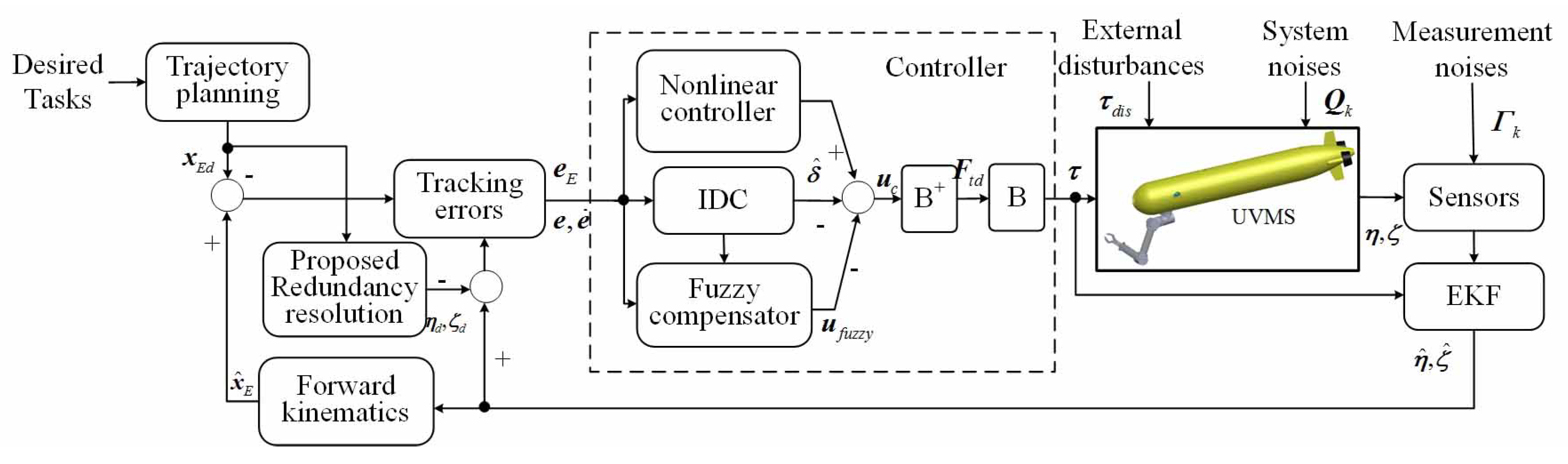
The proposed control system is schematically represented by a block diagram in Figure 4. The controller block includes five sub blocks to calculate a control vector; i.e., the tracking controller, IDC, fuzzy compensator, and blocks. In addition to system dynamics, the tracking controller also requires tracking errors of end-effector positions and joint-space states. The end-effector position tracking errors are calculated according to the desired end-effector positions derived from the trajectory planning block and the estimated end-effector positions obtained from the forward kinematics block using the estimated joint-space states. The estimates of joint-space states are obtained from the EKF block. The proposed redundancy resolution block generates the required joint-space trajectories for the desired tasks. The IDC block estimates the lumped uncertainties and disturbances of the system. The fuzzy compensator reduces the influences of perturbation on the UVMS.
4.5. Stability Analysis
We define a Lyapunov function which is positive definite as:
Differentiating yields
where is assumed to be constant.
Substituting the proposed control law (31) in (22), and taking into account (29), (34) can be rewritten as
By choosing large enough values of , small values of and small enough values of such that
is negative semi-definite, where is a vector with smaller positive values. Consequently, the tracking errors and estimated errors of the system all converge to zero asymptotically; i.e.,
Therefore, the closed-loop system is asymptotically stable in the entire state space.
5. Simulation Studies
To verify the performance of the proposed technique, numerical simulations were performed on a UVMS with a torpedo-type AUV and a 3-DOF underwater manipulator [15] shown in Figure 1. The AUV is driven by five thrusters in total and its thruster configuration is shown in Figure 5. The thruster configuration matrix and its pseudo inverse are shown in the Appendix A. The parameters for the AUV and manipulator are given in the Appendix A and Table 3 and Table 4. From Table 4, it can be seen that the whole system is neutrally buoyant, while the manipulator’s links have negative buoyancy. Thus, the UVMS used for numerical simulations in this paper can approximate to the real system.
5.1. Simulation Conditions
In the simulations, the UVMS’s end-effector is commanded to follow a spatial circle with diameter m and a straight line of length m. The simulation time of the circular trajectory is 50 s, where the initial 10 s is used for acceleration, 30 s is used to follow the circle and the final 10 s is used for deceleration. The simulation time of the straight-line trajectory is 30 s, where in the initial 10 s the acceleration is a half-period sine function, and then it maintains zeros, and in the final 10 s it is a half-period negative sine function. The UVMS’s end-effector maintains orientation during the two trajectory tracking tasks. The initial desired positions and orientations are the same as the initial actual positions and orientations. The initial desired and actual velocities and accelerations are zeros. The average speeds of the two trajectories both are . The sampling time for the simulation is ms.
In this case, the model uncertainties, external disturbances, payload and sensory noises in position and orientation measurements are introduced for simulating the real working environment. To reflect the uncertainties, it is assumed that the modeling inaccuracy for each parameter is . The vector of time-varying ocean currents in the inertial frame is assumed to be governed by (38). It is supposed that the end-effector of the manipulator is attached with a payload of (in water). The following sensory noises are introduced: gaussian noise of mean and standard deviation for the vehicle position measurements; mean and standard deviation for the vehicle attitude measurements; and mean and standard deviation for the manipulator’s joint position measurements. In addition, the thruster dynamic characteristics are inserted into the simulation. Suppose that the thruster response delay time is , and its efficiency is .
To implement solution (7), the primary task vector is . and for the two trajectories. Other parameters are shown in Table 5. A secondary task is designed to align the vehicle orientation and the joint position with the primary task in terms of reducing the coupling effects, as shown in (39).
where is the linear part of .
The distribution matrix is defined as
To illustrate the effectiveness of the proposed redundancy resolution technique in terms of energy savings, the comparative redundancy resolution technique is given in (41).
where the difference between (7) and (41) is that the secondary task vector is not included in the compared technique.
The proposed control scheme is compared with the H∞-EKF method [23] which is given by
where and are the derivative and the proportional gain matrices. and are the estimated vectors from EKF. is the disturbance estimation from EKF as well. is the given positive definite matrix.
For simple representation, the proposed redundancy resolution is termed case 1 (c1), and the comparative redundancy resolution is termed case 2 (c2). Hence, the proposed control scheme based on the proposed redundancy resolution is termed proposed controlc1; the H∞-EKF method based on the proposed redundancy resolution is termed H∞-EKFc1; and the proposed control based on the comparative redundancy resolution is termed proposed controlc2.
5.2. Results and Discussion
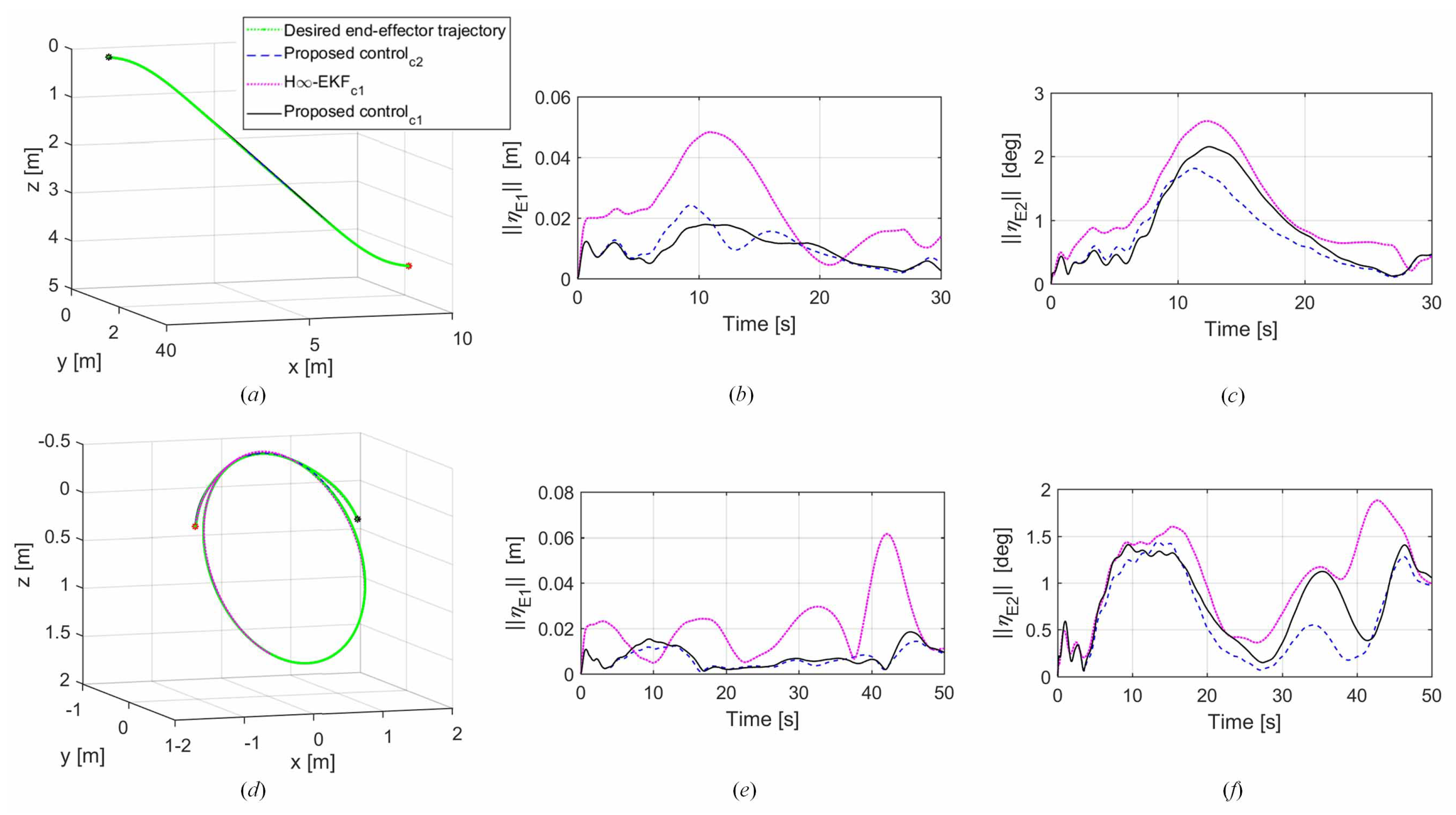
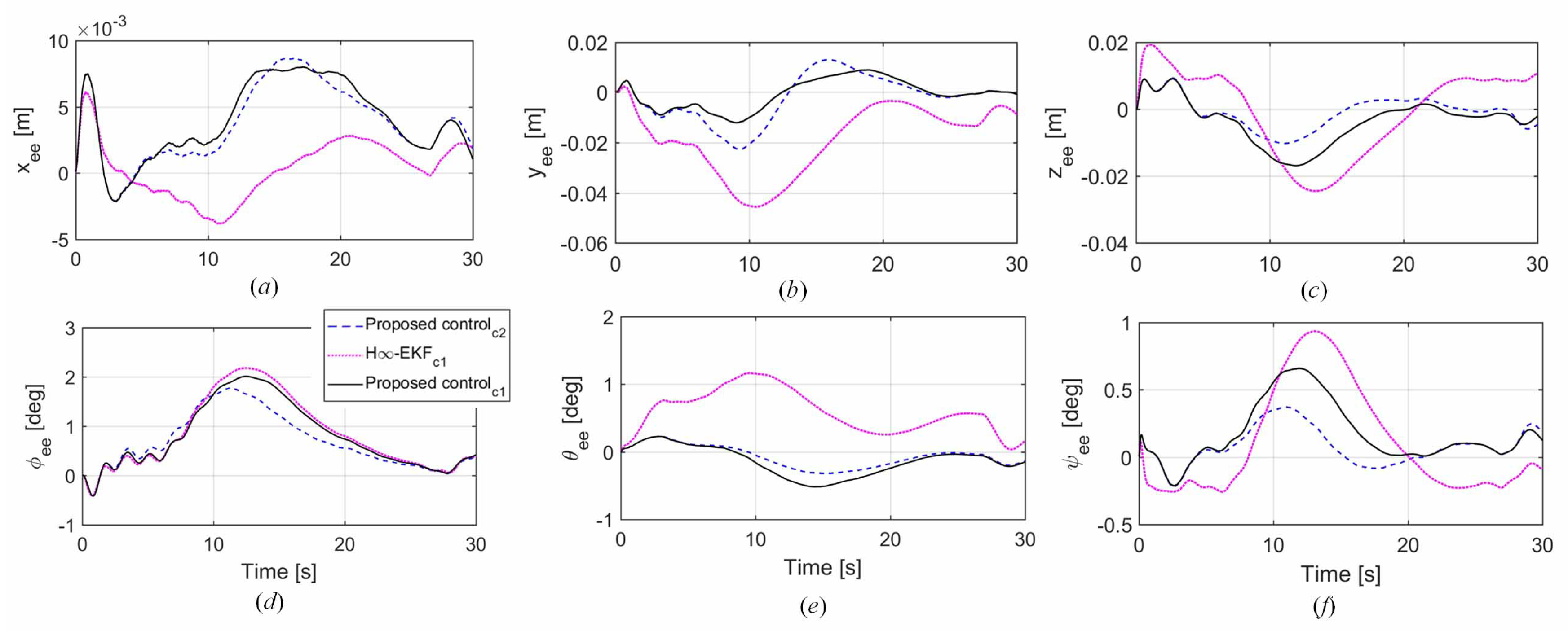
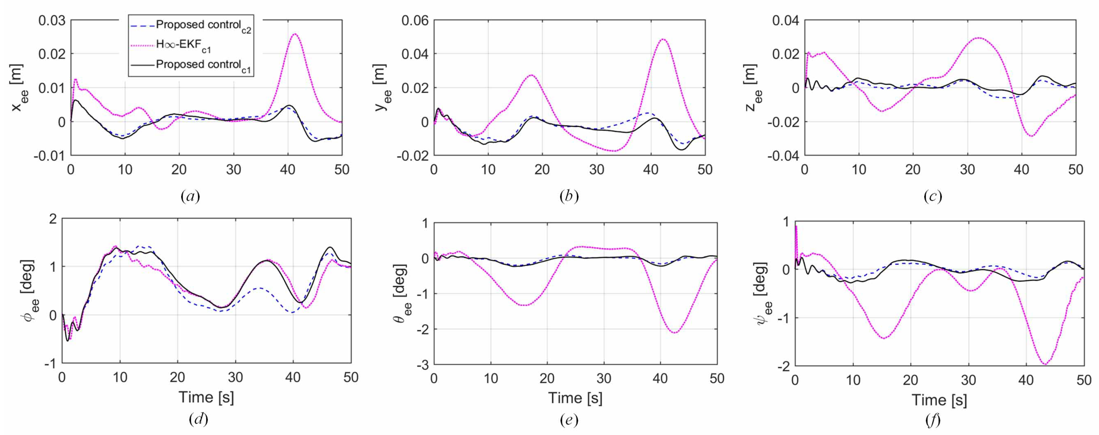
The results of numerical simulations are shown in Figure 6, Figure 7, Figure 8, Figure 9, Figure 10, Figure 11, Figure 12 and Figure 13. Figure 6, Figure 7 and Figure 8 present the desired and actual spatial trajectories and their tracking errors. From these results it is observed that the proposed controller drives the UVMS to track the desired spatial linear and circular trajectories quite satisfactorily in both the proposed redundancy resolution technique (c1) and the comparative redundancy resolution technique (c2). Moreover, the proposed control scheme outperforms the H∞-EKF method, and has smaller tracking errors in both positions and orientations under the conditions of model uncertainties, time-varying ocean currents, payload and sensory noises. Even though the H∞-EKF method adopted a H∞ robust controller to compensate the estimated bias from the EKF, the residual tracking errors can not be fully eliminated, as shown in Figure 6b,c and Figure 6e,f. The proposed controller performs better than the H∞-EKF method in terms of robustness, which is dedicated to the IDC and fuzzy compensator for reducing the perturbation effects.
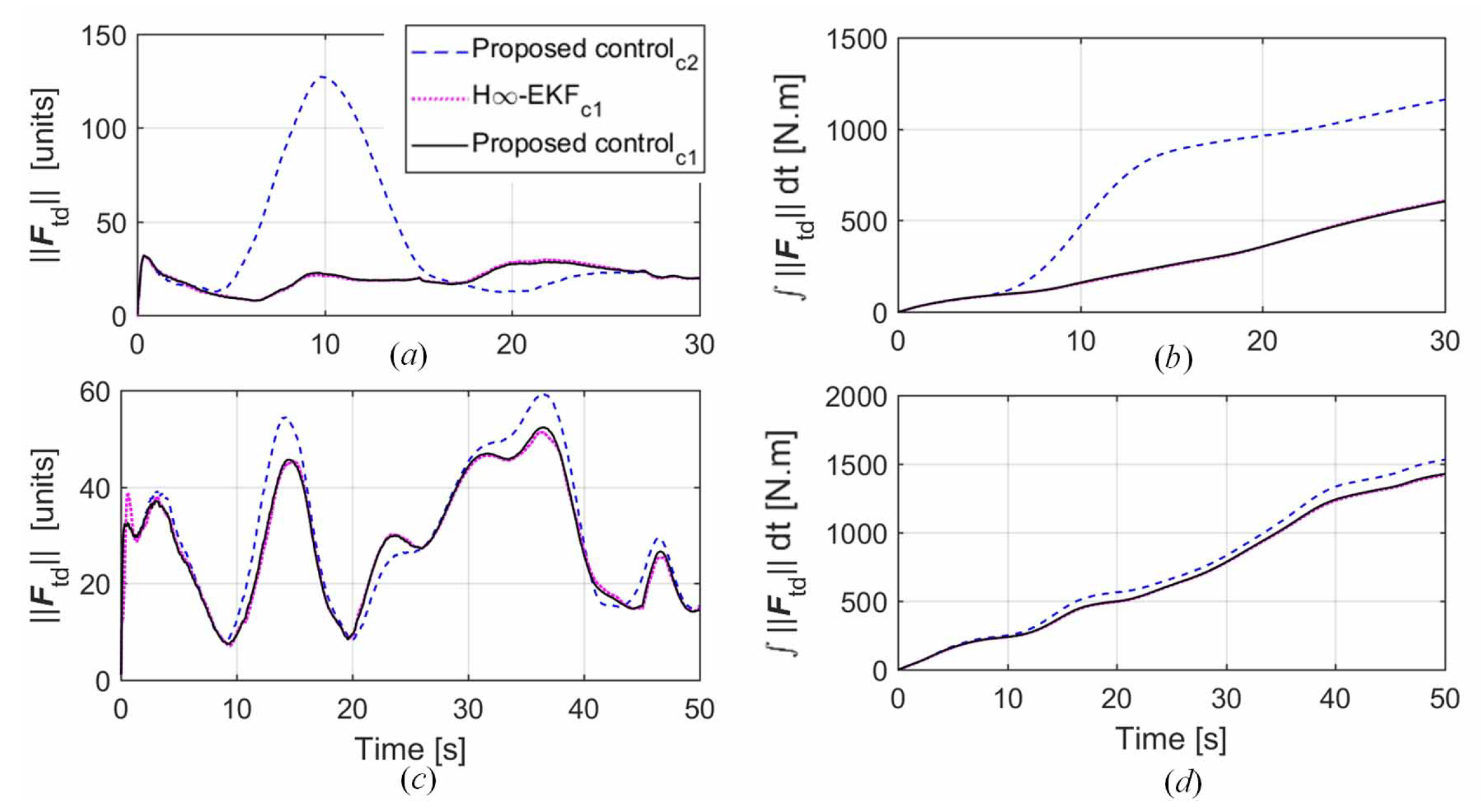
Figure 9 plots the norm of the vector (i.e., thruster forces and actuator torques) and energy consumption of the UVMS. It can be noted that the comparative redundancy resolution technique (c2) is consuming more energy in generating trajectories for the vehicle and manipulator during both the linear and circular trajectories tracking. However in the proposed redundancy resolution technique (c1), the UVMS states are adjusted by self-motion to minimize interaction effects between the vehicle and the manipulator. This is because of the introduction of the secondary task vector and the nonlinear function.
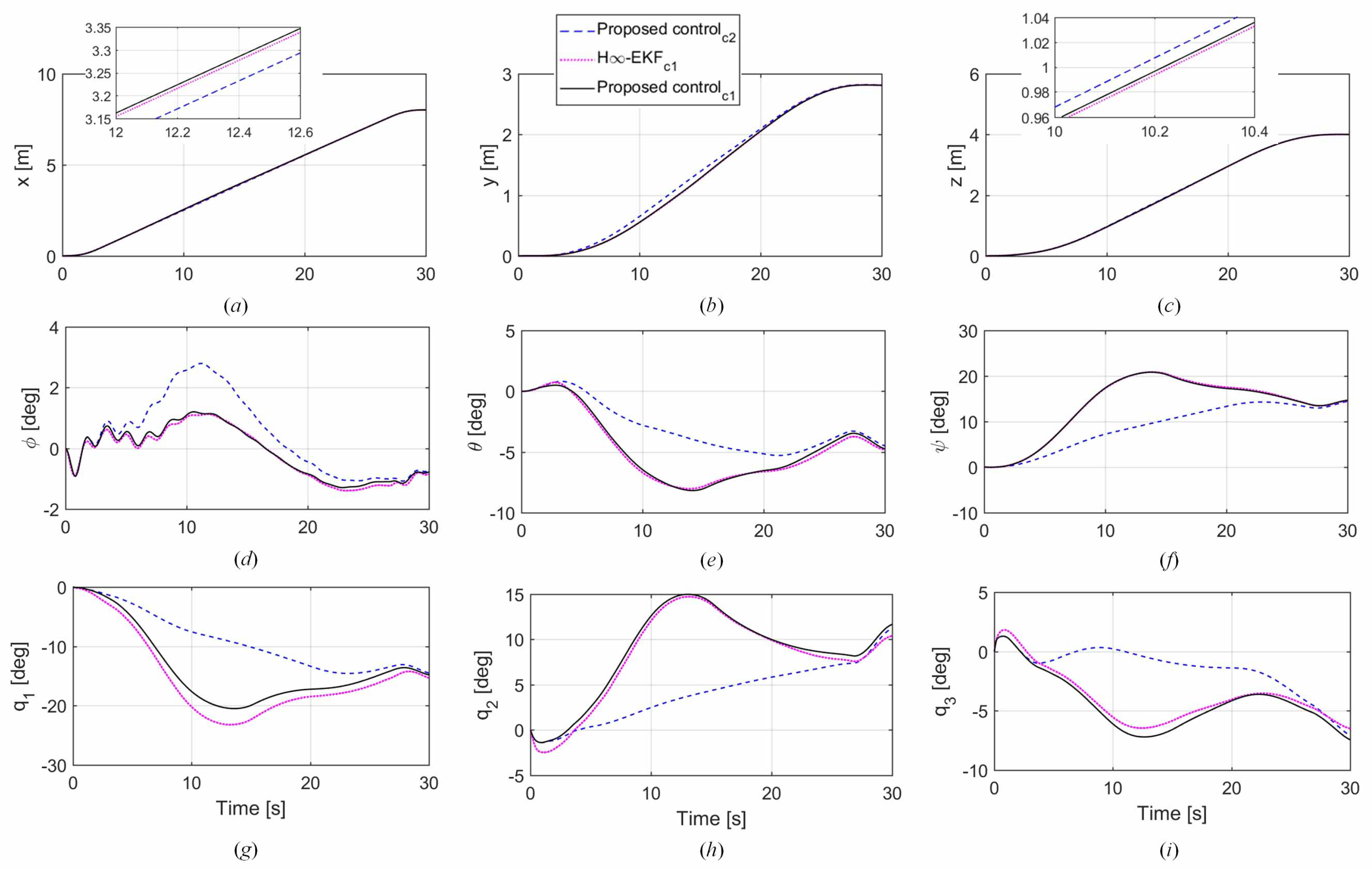
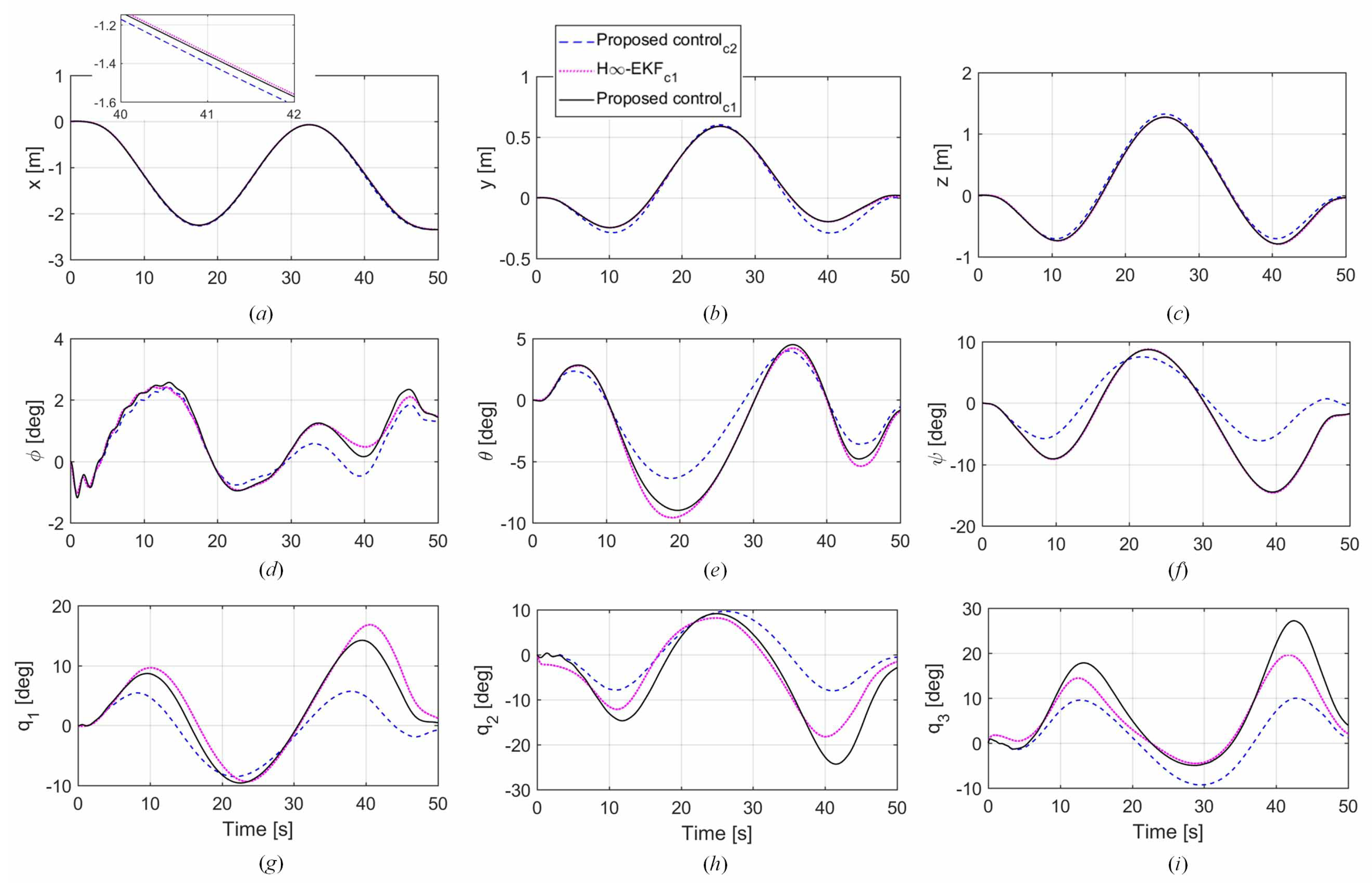
For better understanding, the generated trajectories for the vehicle positions/attitudes and manipulator positions are presented in Figure 10 and Figure 11. It can be seen from the results that the generated trajectories have larger differences on vehicle attitudes and joint angles than vehicle positions. This is because the adjustment of the vehicle position has little effect on reducing the interactive forces between the vehicle and the manipulator without affecting the primary task. Consequently, the energy consumption can be reduced by changing the vehicle attitude and joint angles. In addition, it is observed from Figure 10 and Figure 11 that the small roll and pitch angles of the vehicle are kept in the proposed control scheme, which contributes to properly working of the vehicle’s onboard sensors.
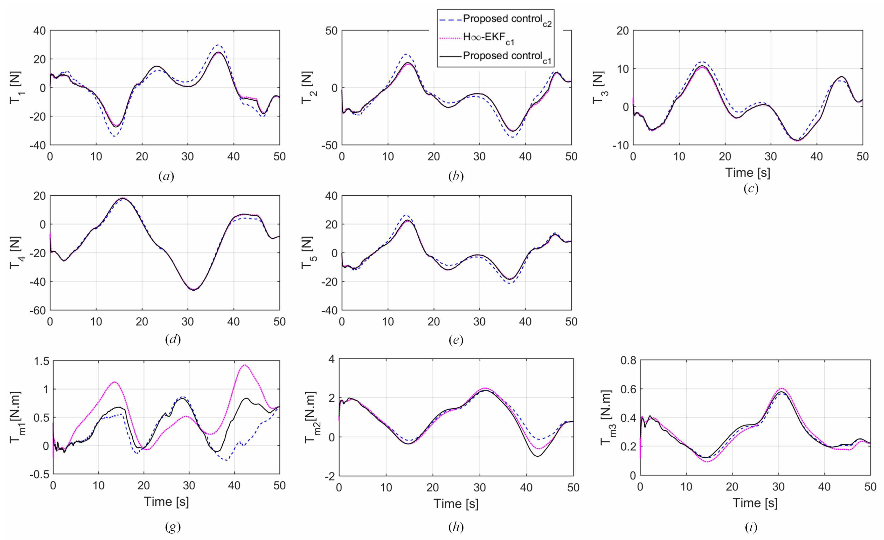
Figure 12 and Figure 13 show the required thruster forces for the vehicle and actuator torques for the manipulator during the linear and circular trajectory tracking. It is observed that the thruster forces for the two trajectories are less in the proposed redundancy resolution technique (c1), which results in the reduced energy consumption. In addition, the thruster forces and actuator torques for both trajectories in the proposed controlc1 are within their constraints ( N for the thrusters and N·m for the actuators).
The quantitative indexes of the time integral of tracking errors and energy consumption are listed in Table 6. From these indices, it is indicated that the tracking error in the proposed controlc1 is smaller than that in the H∞-EKFc1 method, and the energy consumption in the proposed controlc1 is less than that in the proposed controlc2. Overall, the proposed control scheme based on the proposed redundancy resolution technique (c1) ensures the precise and robust performance with a reduced energy requirement under the conditions of model parameter uncertainties, time-varying ocean currents, payload and sensory noises.
In the simulations, we have taken the model parameter uncertainties, time-varying external disturbances, payload and sensory noises into consideration. However, in a practical case, these lumped uncertainties and disturbances may be more complicated, and hence can not be simulated. Even though the results from computer simulations are promising, it is necessary to validate the effectiveness of the proposed control scheme and the proposed redundancy resolution technique through experiments in a water pool or at sea. This is our future work.
6. Conclusions
This paper presents a motion planning and coordinated control scheme for the trajectory tracking of the UVMS. A new secondary task with a nonlinear coefficient for redundancy resolution of the UVMS is proposed. In this way, the interactive effects between the vehicle and the manipulator can be minimized and the energy consumption of the UVMS is reduced. Simulation results show that the energy consumption based on the proposed redundancy resolution technique (proposed controlc1) is reduced by 48% (in the linear trajectory tracking) and 6% (in the circular trajectory tracking), compared with the comparative redundancy resolution technique (proposed controlc2). The proposed redundancy resolution technique is simple in design and easy to implement. Furthermore, a control scheme including a fuzzy compensator and a tracking control with joint-space errors, end-effector errors and inertial delay control (IDC) is proposed. The proposed control scheme ensures precise and robust tracking performance in the presence of model uncertainties, time-varying ocean currents, payload and sensory noises. Simulation results show that the position and orientation tracking precisions based on the proposed controlc1 are reduced by and (in the linear trajectory tracking) and and (in the circular trajectory tracking), compared with the H∞−EKFc1 method [23]. Even though the effectiveness of the proposed redundancy resolution technique and coordinated motion control scheme were validated through numerical simulations, experiments should be carried out on the real UVMS to further enhance the computer simulation results, which will be done in the future.
Author Contributions
Conceptualization, H.H., Y.W. and X.Y.; data curation, H.H.; formal analysis, H.H.; funding acquisition, Y.W. and X.Y.; investigation, H.H.; methodology, H.H.; project administration, Y.W. and X.Y.; resources, Y.W. and W.L.; software, H.H.; supervision, Y.W., X.Y. and W.L.; validation, H.H., Y.W., X.Y. and W.L.; visualization, H.H.; writing—original draft, H.H.; writing—review editing, Y.W. and X.Y. All authors have read and agreed to the published version of the manuscript.
Funding
This research was supported by the National Natural Science Foundation of China under grant number 41876100, in part by the National key research and development program of China under grant number 2017YFC0306001, in part by the Heilongjiang Natural Science Foundation under grant number E2017024 and in part by the Key Program for International S and T Cooperation Projects of China under grant number 2014DFR10010.
Acknowledgments
The authors would like to thank Shuai Li, Fan Zhang and Shitong Du, who provided insight and expertise that greatly assisted the writing of this manuscript.
Conflicts of Interest
The authors declare no conflict of interest. The funders had no role in the design of the study; in the collection, analyses or interpretation of data; in the writing of the manuscript, or in the decision to publish the results.
Appendix A. Simulation Data of the AUV
For the torpedo-type AUV, its center of buoyancy (CB) is , its center of gravity (CG) is and its moment of inertia is . The AUV is equipped with an underwater manipulator, and the manipulator’s base position is . Some model parameters of the AUV given in (3) are composed of rigid-body terms and hydrodynamic terms [42], as shown in the following equations.
where and are the rigid-body terms which represent the inertia matrix and the Coriolis and centripetal matrix. , , and are the matrices related to the hydrodynamic forces. and are the added mass matrix and the added Coriolis and centripetal matrix. and are the quadratic damping matrix and the lift matrix. , , and are given in the following equations [15].
To obtain the above hydrodynamic coefficients, the strip theory is utilized for numerical calculation, where the fluid density is assumed to be , the linear-skin coefficient is assumed to be and the drag coefficient is assumed to be 1. Moreover, some of the obtained coefficients are adjusted based on comparisons with data of the REMUS AUV according to dynamic similarity [15]. Then, the adjusted hydrodynamic coefficients are shown in Table A1.

Table A1.
The list of AUV coefficients.
| - | |||||
For the AUV, the thruster configuration matrix and its pseudo inverse are given as
where , , , , .
References
- Podder, T.K.; Sarkar, N. Unified Dynamics-based Motion Planning Algorithm for Autonomous Underwater Vehicle-Manipulator Systems (UVMS). Robotica 2004, 22, 117–128. [Google Scholar] [CrossRef] [Green Version]
- Antonelli, G.; Chiaverini, S. Fuzzy redundancy resolution and motion coordination for underwater vehicle-manipulator systems. IEEE Trans. Fuzzy Syst. 2003, 11, 109–120. [Google Scholar] [CrossRef]
- Antonelli, G.; Chiaverini, S. Task-priority redundancy resolution for underwater vehicle-manipulator systems. In Proceedings of the IEEE International Conference on Robotics and Automation, Leuven, Belgium, 20 May 1998; pp. 768–773. [Google Scholar]
- Sarkar, N.; Podder, T.K. Coordinated motion planning and control of autonomous underwater vehicle-manipulator systems subject to drag optimization. IEEE J. Ocean. Eng. 2001, 26, 228–239. [Google Scholar] [CrossRef]
- Han, J.; Park, J.; Chung, W.K. Robust coordinated motion control of an underwater vehicle-manipulator system with minimizing restoring moments. Ocean Eng. 2011, 38, 1197–1206. [Google Scholar] [CrossRef]
- Siciliano, B.; Slotine, J.-J.E. A general framework for managing multiple tasks in highly redundant robotic systems. In Proceedings of the Fifth International Conference on Advanced Robotics, Pisa, Italy, 19–22 June 1991; pp. 1211–1216. [Google Scholar]
- Antonelli, G.; Chiaverini, S. A fuzzy approach to redundancy resolution for underwater vehicle-manipulator systems. Control Eng. Pract. 2003, 11, 445–452. [Google Scholar] [CrossRef]
- Wang, Y.; Jiang, S.; Yan, F.; Gu, L.; Chen, B. A new redundancy resolution for underwater vehicle—Manipulator system considering payload. Int. J. Adv. Robot. Syst. 2017, 14. [Google Scholar] [CrossRef]
- Haugalokken, B.O.A.; Joergensen, E.K.; Schjolberg, I. Experimental validation of end-effector stabilization for underwater vehicle-manipulator systems in subsea operations. Robot. Auton. Syst. 2018, 109, 1–12. [Google Scholar] [CrossRef] [Green Version]
- Tang, C.; Wang, Y.; Wang, S.; Wang, R.; Tan, M. Floating Autonomous Manipulation of the Underwater Biomimetic Vehicle-Manipulator System: Methodology and Verification. IEEE Trans. Ind. Electron. 2018, 65, 4861–4870. [Google Scholar] [CrossRef]
- Simetti, E.; Casalino, G.; Wanderlingh, F.; Aicardi, M. Task priority control of underwater intervention systems: Theory and applications. Ocean Eng. 2018, 164, 40–54. [Google Scholar] [CrossRef]
- Youakim, D.; Ridao, P. Motion planning survey for autonomous mobile manipulators underwater manipulator case study. Robot. Auton. Syst. 2018, 107, 20–44. [Google Scholar] [CrossRef]
- Mcmillan, S.; Orin, D.E.; Mcghee, R.B. Efficient dynamic simulation of an underwater vehicle with a robotic manipulator. IEEE Trans. Syst. Man Cybern. 1995, 25, 1194–1206. [Google Scholar] [CrossRef] [Green Version]
- Dannigan, M.W.; Russell, G. Evaluation and reduction of the dynamic coupling between a manipulator and an underwater vehicle. IEEE J. Ocean. Eng. 1998, 23, 260–273. [Google Scholar] [CrossRef]
- Han, H.; Wei, Y.; Ye, X.; Liu, W. Modelling and Fuzzy Decoupling Control of an Underwater Vehicle-Manipulator System. IEEE Access 2020, 8, 18962–18983. [Google Scholar] [CrossRef]
- Schjolberg, I.; Fossen, T.I. Modelling and Control of Underwater Vehicle-Manipulator Systems. In Proceedings of the 3rd Conference on Marine Craft Maneuvering and Control, Southampton, UK, 7–9 September 1994; pp. 45–57. [Google Scholar]
- Taira, Y.; Sagara, S.; Oya, M. Model-based motion control for underwater vehicle-manipulator systems with one of the three types of servo subsystems. Artif. Life Robot 2019, 6, 1–16. [Google Scholar] [CrossRef]
- Korkmaz, O.; Ider, S.K.; Ozgoren, M.K. Trajectory Tracking Control of an Underactuated Underwater Vehicle Redundant Manipulator System. Asian J. Control 2016, 18, 1593–1607. [Google Scholar] [CrossRef]
- Cai, M.; Wang, Y.; Wang, S.; Wang, R.; Ren, Y.; Tan, M. Grasping Marine Products with Hybrid-Driven Underwater Vehicle-Manipulator System. IEEE Trans. Autom. Sci. Eng. 2020. [Google Scholar] [CrossRef]
- Santhakumar, M.; Kim, J. Robust Adaptive Tracking Control of Autonomous Underwater Vehicle-Manipulator Systems. J. Dyn. Syst. Meas. Control 2014, 136, 054502. [Google Scholar] [CrossRef]
- Antonelli, G.; Caccavale, F.; Chiaverini, S. Adaptive Tracking Control of Underwater Vehicle-Manipulator Systems Based on the Virtual Decomposition Approach. IEEE Trans. Robot. Autom. 2004, 20, 594–602. [Google Scholar] [CrossRef]
- Mohan, S.; Kim, J. Indirect adaptive control of an autonomous underwater vehicle-manipulator system for underwater manipulation tasks. Ocean Eng. 2012, 54, 233–243. [Google Scholar] [CrossRef]
- Dai, Y.; Yu, S. Design of an indirect adaptive controller for the trajectory tracking of UVMS. Ocean Eng. 2008, 151, 234–245. [Google Scholar] [CrossRef]
- Esfahani, H.N. Robust Model Predictive Control for Autonomous Underwater Vehicle–Manipulator System with Fuzzy Compensator. Pol. Marit. Res. 2019, 26, 104–114. [Google Scholar] [CrossRef] [Green Version]
- Cai, M.; Wang, Y.; Wang, S.; Wang, R.; Cheng, L.; Tan, M. Prediction-Based Seabed Terrain Following Control for an Underwater Vehicle-Manipulator System. IEEE Trans. Syst. Man Cybern. Syst. 2019. [Google Scholar] [CrossRef]
- Nikou, A.; Verginis, C.K.; Dimarogonas, D.V. A Tube-based MPC Scheme for Interaction Control of Underwater Vehicle Manipulator Systems. In Proceedings of the 2018 IEEE/OES Autonomous Underwater Vehicle Workshop (AUV), Porto, Portugal, 6–9 November 2018; pp. 1–8. [Google Scholar]
- Dai, Y.; Yu, S.; Yan, Y. An Adaptive EKF-FMPC for the Trajectory Tracking of UVMS. IEEE J. Ocean. Eng. 2019, 1–15. [Google Scholar] [CrossRef]
- Dai, Y.; Yu, S.; Yan, Y.; Yu, X. An EKF-Based Fast Tube MPC Scheme for Moving Target Tracking of a Redundant Underwater Vehicle-Manipulator System. IEEE ASME Trans. Mechatron. 2019, 24, 2803–2814. [Google Scholar] [CrossRef]
- Esfahani, H.N.; Azimirad, V.; Danesh, M. A Time Delay Controller included terminal sliding mode and fuzzy gain tuning for Underwater Vehicle-Manipulator Systems. Ocean Eng. 2015, 107, 97–107. [Google Scholar] [CrossRef]
- Hosseinnajad, A.; Loueipour, M. Time Delay Controller Design for Dynamic Positioning of ROVs based on Position and Acceleration Measurements. In Proceedings of the 6th International Conference on Control, Instrumentation and Automation, Sanandaj, Iran, 30–31 October 2019. [Google Scholar]
- Cui, R.; Chen, L.; Yang, C.; Chen, M. Extended State Observer-Based Integral Sliding Mode Control for an Underwater Robot With Unknown Disturbances and Uncertain Nonlinearities. IEEE Trans. Ind. Electron. 2017, 64, 6785–6795. [Google Scholar] [CrossRef] [Green Version]
- Chen, W.H. Disturbance Observer Based Control for Nonlinear Systems. IEEE ASME Trans. Mechatron. 2005, 9, 706–710. [Google Scholar] [CrossRef] [Green Version]
- Chen, W.; Wei, Y.; Zeng, J.; Han, H.; Jia, X. Adaptive Terminal Sliding Mode NDO-Based Control of Underactuated AUV in Vertical Plane. Discret. Dyn. Nat. Soc. 2016. [Google Scholar] [CrossRef] [Green Version]
- Li, J.; Huang, H.; Wan, L.; Zhou, Z.; Xu, Y. Hybrid Strategy-based Coordinate Controller for an Underwater Vehicle Manipulator System Using Nonlinear Disturbance Observer. Robotica 2019, 37, 1710–1731. [Google Scholar] [CrossRef]
- Londhe, P.S.; Dhadekar, D.D.; Patre, B.M.; Waghmare, L.M. Uncertainty and disturbance estimator based sliding mode control of an autonomous underwater vehicle. Intern. J. Dyn. Control 2017, 5, 1122–1138. [Google Scholar] [CrossRef]
- Han, H.; Wei, Y.; Guan, L.; Ye, X.; Wang, A. Trajectory Tracking Control of Underwater Vehicle-Manipulator Systems Using Uncertainty and Disturbance Estimator. In Proceedings of the OCEANS 2018 MTS/IEEE, Charleston, SC, USA, 22–25 October 2018. [Google Scholar]
- Suryawanshi, P.V.; Shendge, P.D.; Phadke, S.B. Robust sliding mode control for a class of nonlinear systems using inertial delay control. Nonlinear Dyn. 2014, 78, 1921–1932. [Google Scholar] [CrossRef]
- Mohan, S.; Kim, J. Coordinated motion control in task space of an autonomous underwater vehicle– manipulator system. Ocean Eng. 2015, 104, 155–167. [Google Scholar] [CrossRef]
- Londhe, P.S.; Santhakumar, M.; Patre, B.M.; Waghmare, L.M. Task Space Control of an Autonomous Underwater Vehicle Manipulator System by Robust Single-Input Fuzzy Logic Control Scheme. IEEE J. Ocean. Eng. 2016, 42, 13–28. [Google Scholar] [CrossRef]
- Londhe, P.S.; Mohan, S.; Patre, B.M.; Waghmare, L.M. Robust task-space control of an autonomous underwater vehicle- manipulator system by PID-like fuzzy control scheme with disturbance estimator. Ocean Eng. 2017, 139, 1–13. [Google Scholar] [CrossRef]
- Antonelli, G. Underwater Robots: Motion and Force Control of Vehicle-Manipulator Systems, 3rd ed.; Springer: Berlin/Heidelberg, Germany, 2013; pp. 52–55. [Google Scholar]
- Fossen, T.I. Handbook of Marine Craft Hydrodynamics and Motion Control; John Wiley and Sons: Hoboken, NJ, USA, 2011; pp. 128–131. [Google Scholar]
Figure 1.
Coordinate systems of the underwater vehicle manipulator system (UVMS).

Figure 2.
Nonlinear function of .

Figure 3.
Input and output membership functions.

Figure 4.
Block diagram of the proposed controller.

Figure 5.
Thruster distribution of the AUV.

Figure 6.
Spatial linear and circular trajectories and their tracking errors. () Desired linear trajectory and tracking control results; (,) position tracking errors in positions and orientations; () desired circular trajectory and tracking control results; (,) tracking errors in positions and orientations.

Figure 7.
End-effector errors when tracking the linear trajectory. () error, () error, () error, () tracking errors in the end-effector roll direction, () tracking errors in the end-effector pitch direction, () tracking errors in the end-effector yaw direction.
Figure 7.
End-effector errors when tracking the linear trajectory. () error, () error, () error, () tracking errors in the end-effector roll direction, () tracking errors in the end-effector pitch direction, () tracking errors in the end-effector yaw direction.

Figure 8.
End-effector errors when tracking the circular trajectory. () error, () error, () error, () tracking errors in the end-effector roll direction, () tracking errors in the end-effector pitch direction, () tracking errors in the end-effector yaw direction.
Figure 8.
End-effector errors when tracking the circular trajectory. () error, () error, () error, () tracking errors in the end-effector roll direction, () tracking errors in the end-effector pitch direction, () tracking errors in the end-effector yaw direction.

Figure 9.
Time histories of the norm of the vector and UVMS energy consumption. (,) Results from the linear trajectory tracking, (,) results from the circular trajectory tracking, (; i.e., the vector of thruster forces and actuator torques).
Figure 9.
Time histories of the norm of the vector and UVMS energy consumption. (,) Results from the linear trajectory tracking, (,) results from the circular trajectory tracking, (; i.e., the vector of thruster forces and actuator torques).

Figure 10.
Joint-space positions for the straight line trajectory. () X position, () y position, () z position, () roll angle, () pitch angle, () yaw angle, () joint 1 angle, () joint 2 angle, () joint 3 angle.
Figure 10.
Joint-space positions for the straight line trajectory. () X position, () y position, () z position, () roll angle, () pitch angle, () yaw angle, () joint 1 angle, () joint 2 angle, () joint 3 angle.

Figure 11.
Joint-space positions for the circular trajectory. () X position, () y position, () z position, () roll angle, () pitch angle, () yaw angle, () joint 1 angle, () joint 2 angle, () joint 3 angle.
Figure 11.
Joint-space positions for the circular trajectory. () X position, () y position, () z position, () roll angle, () pitch angle, () yaw angle, () joint 1 angle, () joint 2 angle, () joint 3 angle.

Figure 12.
Thruster forces and actuator torques for the line trajectory tracking. (–) Thruster forces , , , and ; (–) actuator torques , and .
Figure 12.
Thruster forces and actuator torques for the line trajectory tracking. (–) Thruster forces , , , and ; (–) actuator torques , and .

Figure 13.
Thruster forces and actuator torques for the circular trajectory tracking. (–) Thruster forces , , , and ; (–) actuator torques , and .
Figure 13.
Thruster forces and actuator torques for the circular trajectory tracking. (–) Thruster forces , , , and ; (–) actuator torques , and .

Table 1.
Rule base for .
Table 2.
Relationships between two input variables and an output variable.
Table 3.
D-H parameters of the manipulator.
| Joint (k) | Offset (αk−1) | Length (ak−1) | Distance (dk) | Angle (θk) |
|---|---|---|---|---|
| 1 | 0° | 0 | 0 | q1 |
| 2 | 90° | lq1 | 0 | q2 |
| 3 | 0° | lq2 | 0 | q3 |
| 4 | 0° | lq3 | 0 | q4 = 0° |
Table 4.
The list of UVMS parameters.
Table 5.
Parameters for the proposed redundancy resolution technique.
| 0 | 15 | ||||||
| 45 |
Table 6.
Performance analysis of the UVMS for the linear and circular trajectories tracking.
, , .
© 2020 by the authors. Licensee MDPI, Basel, Switzerland. This article is an open access article distributed under the terms and conditions of the Creative Commons Attribution (CC BY) license (http://creativecommons.org/licenses/by/4.0/).
Share and Cite
MDPI and ACS Style
Han, H.; Wei, Y.; Ye, X.; Liu, W. Motion Planning and Coordinated Control of Underwater Vehicle-Manipulator Systems with Inertial Delay Control and Fuzzy Compensator. Appl. Sci. 2020, 10, 3944. https://doi.org/10.3390/app10113944
AMA Style
Han H, Wei Y, Ye X, Liu W. Motion Planning and Coordinated Control of Underwater Vehicle-Manipulator Systems with Inertial Delay Control and Fuzzy Compensator. Applied Sciences. 2020; 10(11):3944. https://doi.org/10.3390/app10113944
Chicago/Turabian StyleHan, Han, Yanhui Wei, Xiufen Ye, and Wenzhi Liu. 2020. "Motion Planning and Coordinated Control of Underwater Vehicle-Manipulator Systems with Inertial Delay Control and Fuzzy Compensator" Applied Sciences 10, no. 11: 3944. https://doi.org/10.3390/app10113944
Note that from the first issue of 2016, this journal uses article numbers instead of page numbers. See further details here.